The Multiple Phases of Interstellar and Halo Gas
in a Possible Group of Galaxies at $z\sim 1$

Abstract

We used HIRES/Keck profiles ($R\sim 6$ km s^-1) of Mgii and Feii in combination with FOS/HST spectra ($R\sim 230$ km s^-1) to place constraints on the physical conditions (metallicities, ionization conditions, and multiphase distribution) of absorbing gas in three galaxies at $z=0.9254$, $0.9276$, and $0.9343$ along the line of sight to PG $1206+459$. The chemical and ionization species covered in the FOS/HST spectra are Hi, Siii, Cii, Nii, Feiii, Siiii, Siiv, Niii, Ciii, Civ, Svi, Nv, and Ovi, with ionization potentials ranging from 13.6 to 138 eV. The multiple Mgii clouds exhibit complex kinematics and the Civ, Nv and Ovi are exceptionally strong in absorption. We assumed that the Mgii clouds are photoionized by the extra–galactic background and determined the allowed ranges of their physical properties as constrained by the absorption strengths in the FOS spectra. A main result of this paper is that the low resolution spectra can provide meaningful constraints on the physical conditions of the Mgii clouds, including allowed ranges of cloud to cloud variations within a system. We find that the Mgii clouds, which have a typical size of $\sim 100$ pc, give rise to the Siiv, the majority of which arises in a single, very large ($\sim 5$ kpc), higher ionization cloud. However, the Mgii clouds cannot account for the strong Civ, Nv, and Ovi absorption. We conclude that the Mgii clouds are embedded in extended ($10$–$20$ kpc), highly ionized gas that gives rise to Civ, Nv, and Ovi; these are multiphase absorption systems. The high ionization phases have near–solar metallicity and are consistent with Galactic–like coronae surrounding the individual galaxies, as opposed to a very extended common “halo” encompassing all three galaxies.

1. Introduction

An ultimate goal of the study of quasar (QSO) absorption lines is to develop a comprehensive understanding of the kinematic, chemical, and ionization conditions of gaseous structures in early–epoch galaxies and to chart their cosmic evolution. For a comprehensive physical picture of any given absorption system, both high resolution spectra of a wide range of chemical and ionization species and the empirically measured properties of the associated galaxies are required. For $z\sim 1$, shortly following the epoch of peak star formation, the association between Mgii $\lambda\lambda 2796,2803$ absorption and galaxies is well established (Bergeron & Boissé (1991); Steidel (1995)), and their kinematics, though complex and varied, are consistent with being coupled to the galaxies themselves (Churchill, Steidel, & Vogt (1996); Charlton & Churchill (1998)). It is unfortunate, however, that for $z\sim 1$, the spectroscopic data of are not of uniform, high quality due to the need for large amounts of space–based telescope time to observe ultraviolet wavelengths. Presently, any comprehensive analyses of low redshift systems for which the low ionization species (i.e. Mgii, Feii, Mgi) have been observed at high resolution with HIRES/Keck (see Churchill, Vogt, & Charlton 1999b) must incorporate low resolution FOS/HST spectra of the intermediate and high ionization species, especially the strong Civ $\lambda\lambda 1548,1550$, Nv $\lambda\lambda 1238,1242$, and Ovi $\lambda\lambda 1031,1037$ doublets, and of several other important low ionization species.

Presently, it is not clear if these low resolution data can be used to place meaningful constraints on the chemical and ionization conditions of the clouds in Mgii selected absorbers. In this paper, we investigated this issue in a pilot study, since an affirmation would imply that a larger sample could be studied using existing data from the HST Archive. We would then be able to address the broader implications for galaxy formation scenarios based upon the inferred metallicities, abundance patterns, and inferred relative spatial distribution of the low and high ionization absorbing gas clouds.

Figure 1.— The HIRES/Keck Mgii $\lambda\lambda 2796,2803$ doublet profiles at $R=45,000$. Three systems, A, B, and C, have been identified at $z_{A}=0.92540$, $z_{B}=0.92760$, and $z_{C}=0.93428$. The labeled bar bar ticks give the systemic redshifted wavelengths for the Mgii doublets in these systems. The solid line through the data is a synthetic spectrum from a Voigt profile decomposition. The vertical ticks above the continuum give the locations of the Voigt profile components.

Under the assumptions of photoionization and/or collisional ionization equilibrium, we developed a technique in which it was assumed that the number of clouds and their kinematics are obtained by Voigt profile decomposition of the high resolution Mgii spectra. We then used the lower resolution profiles from the FOS data to place constraints on the range of chemical and ionization conditions in these clouds. We also explored the idea that the Mgii could arise in relatively low ionization clouds embedded in a higher ionization and more extended medium (see Bergeron et al. (1994); Churchill 1997a ). More specifically, we set out to answer three questions: (1) Assuming the Mgii clouds measured with HIRES are photoionized, can we construct model clouds that are consistent with the many low and intermediate ionization species captured in the FOS data? (2) If so, are we required to infer an additional (presumedly low density and diffuse) component to account for higher ionization absorption from Civ, Nv, and Ovi? (3) If so, can this diffuse component be made consistent with photoionized only, collisionally ionized only, or photo plus collisionally ionized gas?

For this paper, we chose the three systems at $z_{\rm abs}=0.9254$, $0.9276$, and $0.9343$ along the line of sight toward PG $1206+459$ ($z_{\rm em}=1.16$) because they are exceptionally rich in low, intermediate, and high ionization ultraviolet transitions (Burles & Tytler (1996); Churchill 1997b ; Jannuzi et al. (1998)). The HIRES/Keck Mgii profiles are illustrated in Figure 1. Two of the systems are kinematically “complex” and are separated by $\sim 300$ km s^-1. The third system is more isolated, being $\sim+1000$ km s^-1 from the other two. This system is classified as a “weak” Mgii absorber [defined by $W_{\rm r}(2796)<0.3$ Å (Churchill et al. 1999a )]. The highest ionization transitions, Civ, Nv and Ovi, are seen to have a total kinematic spread of $\sim 1000$ km s^-1 coincident with the three system seen in Mgii absorption (Churchill 1997b ).

In the QSO field, Kirhakos et al. (1994) found three bright galaxies with angular separations from the quasar of 5.6, 8.6, and 9.0″ and $g$ magnitudes 21.1, 21.5, and 22.3, respectively. The 8.6″ galaxy has detected [Oii] $\lambda 3727$ with flux $9\times 10^{-17}$ ergs cm^-2 s^-1 at $z=0.93$ (Thimm (1995)). At this redshift, the QSO–galaxy impact parameters are $29$, $45$, and $47~{}h^{-1}$ kpc ($q_{0}=0.05$). There are $\sim 10$ galaxies with $21\leq g\leq 22$ within 100″ of the QSO (Kirhakos et al. (1994)). This is an overdensity by a factor of $\sim 3$ compared to field galaxies (Tyson (1988)). Thus, it is of interest to entertain the possibility of a group environment for these absorbers.

In § 2 we describe the data and its analysis. In § 3 we outline our modeling technique and simplifying assumptions. A synopsis of the model results are given in § 4. Details on how the data were used to constrain the models and how various ionizing spectral energy distributions modify these models are given in Appendices A and B. In § 5, we compare and contrast the system properties, and in § 6, we discuss what might be inferred about the relative spatial distribution of the low and high ionization gas. We summarize in § 7.

2. Data and Analysis

2.1. HIRES/Keck

The optical data were obtained with the HIRES spectrometer (Vogt et al. (1994)) on the Keck I telescope on 23 January 1995 UT under clear and stable conditions with a seeing of $\sim 0.6$″. The spectral resolution is $\sim 6.6$ km s^-1 ($R=45,000$), with a sampling of 3 pixels per resolution element. The signal–to–noise ratio is $\sim 50$ per resolution element. The Feii $\lambda 2344$, $2374$, $2383$, $2587$, and $2600$ transitions were captured at similar signal–to–noise ratio.

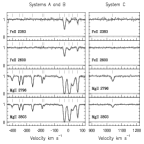
Figure 2.— The kinematics of the Mgii systems are shown, with individual clouds seen in Feii $\lambda 2383$, Feii $\lambda 2600$, Mgii $\lambda 2796$, and Mgii $\lambda 2803$ absorption aligned in rest–frame velocity. Systems A and B are shown together in the left panel and system C is shown in the right panel. The zero–point is defined at $z=0.92760$. The solid lines through the data are synthetic spectra from a Voigt profile decomposition. The ticks above the continuum give the locations of the Voigt profile components.

The HIRES spectrum was reduced with the IRAF Apextract package for echelle data. The detailed steps for the reduction are outlined in Churchill (1995). The spectrum was extracted using the optimized routines of Horne (1986) and Marsh (1989). The wavelengths were calibrated to vacuum using the IRAF task ecidentify, which models the full 2D echelle format. The absolute wavelength scale was then corrected to heliocentric velocity. The continuum normalization was performed using the IRAF sfit task. Objective and unbiased identification of absorption features (without regard to their association with the studied systems) was performed as described in Churchill et al. (1999b), using the methodology of Schneider et al. (1993).

Three systems, which we hereafter call A, B, and C, are observed at redshifts $z_{A}=0.92540$, $z_{B}=0.92760$, and $z_{C}=0.93428$. In Figure 1, we present the Mgii doublet profiles. The doublets are marked by the labeled bar above the normalized continuum. The solid curve through the data is a model spectrum generated using Voigt profile (VP) decomposition. The free parameters are the number of VP components (“clouds”) and, for each, its redshift, column density, and Doppler $b$ parameter. We have used the program MINFIT (Churchill 1997c ), which performs a $\chi^{2}$ minimization while minimizing the number of clouds using a specified confidence level and the standard F–test. The adopted VP decomposition had six clouds in system A, five clouds in system B, and a single cloud in system C.

The HIRES data and the VP decompositions are shown in Figure 2 with the profiles aligned in rest–frame velocity. In Table 1, we present the cloud properties, including individual redshifts, velocities with respect to $z=0.92760$, column densities, $b$ parameters, and the ratios $\log\{N({\hbox{{\rm Fe}\kern 1.00006pt{\sc ii}}})/N({\hbox{{\rm Mg}\kern 1.00006pt{\sc ii}}})\}$. Only system B was found to have measurable Feii. The $1\sigma$ upper limits on Feii were obtained for each cloud from the equivalent width limits of the $\lambda 2600$ transition. For Feii in system A, we measured a mean $1\sigma$ column density upper limit of $N({\hbox{{\rm Fe}\kern 1.00006pt{\sc ii}}})\leq 10^{11.1}$ cm^-2 for the six clouds using the technique of stacking (Norris, Hartwick, & Peterson (1983)).

dummy space.

2.2. FOS/HST

The ultraviolet data were obtained with the Faint Object Spectrograph (FOS) on the Hubble Space Telescope as part of the QSO Absorption Line Key Project. The data acquisition, their reduction, and the objective absorption line lists are presented in Jannuzi et al. (1998). Their fully reduced G190H and G270H spectra have kindly been made available for this study. The spectra have a resolution of $R=1300$ ($\sim 230$ km s^-1) and cover the approximate wavelength intervals $1600$ to $2313$ Å and $2225$ to $3280$ Å for the G190H and G270H settings, respectively.

For the most part, we have adopted the Key Project continuum fits and line identifications. Some refinement was needed near the Siiv $\lambda\lambda 1393,1402$ doublet ($2680\leq\lambda_{\rm obs}\leq 2715$ Å on G270H), which lies on the red wing of the broad Ly$\alpha$ emission line, and near the Siii $\lambda\lambda 1190,1193$ doublet ($2290\leq\lambda_{\rm obs}\leq 2310$ Å on G190H), which lies at the spectrum edge. We have re–fit the continuum across these regions.

A Lyman limit break is present at $\sim 1760$ Å (however, see Stengler–Larrea 1995; Jannuzi et al. 1998). We extrapolated the continuum fit of Jannuzi et al. below the break starting at the break shoulder ($\lambda=1895$ Å). This technique preserved the measured optical depth, or the break ratio, $F_{+}/F_{-}$ (Schneider et al. (1993)), while yielding a reasonable approximation to the shape of the recovery (see Figure 3$a$). Due to the high density of lines, the Jannuzi et al. continuum may have been systematically low by 5–10% in the region 1790 to 1820 Å and our extrapolation may have propagated this systematic offset. Nonetheless, this error has a negligible effect on the measured break ratio of $2.5\pm 0.4$, which we obtained from the unnormalized as well as the normalized spectrum. This ratio implies $\tau_{\rm LL}\simeq 0.9$ and a total neutral hydrogen column density of $N({\hbox{{\rm H}\kern 1.00006pt{\sc i}}})\simeq 10^{17.2}$ cm^-2.

Out of the $\sim 70$ QSOs analyzed by the QSO Absorption Line Key Project, PG $1206+459$ is one of eight for which the line identifications (IDs) were subject to greater uncertainty (the Ly$\alpha$ forest is ubiquitous blueward of 2623 Å and at least four metal systems are present). Using the HIRES data for cross checks with the Jannuzi et al. line IDs in the FOS spectrum, we have made a table of transitions, including those detected and those used for constraining the models. In Table 2 (end of paper), we have listed the observed wavelengths, line IDs, ionization potentials, and notes on any blending. For example, we identified the Lyman series down to Ly$\epsilon$, beyond which the three systems blend together. The FOS spectrum provides a large number of chemical and ionization species, including Ly$\alpha$, Ly$\beta$, Ly$\gamma$, Ly$\delta$, Ly$\epsilon$, Cii $\lambda 1036$ and $\lambda 1334$, Ciii $\lambda 977$, Civ $\lambda\lambda 1548,1550$, Nii $\lambda 915$, Niii $\lambda 989$, Nv $\lambda\lambda 1238,1242$, Ovi $\lambda\lambda 1031,1037$, Siii $\lambda\lambda 1190,1193$ and $\lambda 1260$, Siiii $\lambda 1206$, Siiv $\lambda\lambda 1393,1402$, and Svi $\lambda\lambda 933,944$. These species represent a wide range of ionization potentials from 13.6 eV for Hi to 138.1 eV for Ovi.

3. The Models

Assuming the Mgii clouds are photoionized, our goal was to determine if we can obtain useful constraints on their range of chemical and ionization conditions using the FOS/HST spectra. Within this context, we also explored the possibility of a high ionization (Civ, Nv, and Ovi), presumedly diffuse, component. In principle, this high ionization phase could be photoionized, collisionally ionized, or photo plus collisionally ionized gas (a spatially segregated two–phase high ionization component).

For both the Mgii clouds and the high ionization phase, the extragalactic ultraviolet ionizing background spectrum of Haardt & Madau (1996) for $z=1$ was assumed. Using the [Oii] $\lambda 3727$ detection and constraints measured by Thimm (1995), we explored the range of allowed contributions (modifications to the Haardt & Madau background) from various galactic spectral energy distributions. We find that galactic contributions, within the allowed ranges explored, do not modify general conclusions based upon the assumption of a pure Haardt & Madau background (see Appendix B).

3.1. The Mgii Clouds

We used the photoionization code CLOUDY (version 90.4; Ferland (1996)). The free parameters are the neutral hydrogen column density, $N({\hbox{{\rm H}\kern 1.00006pt{\sc i}}})$, the metallicity, $Z$, the abundance pattern, and the ionization “parameter”, $U$, which is defined as the ratio of the number of hydrogen ionizing photons to the hydrogen number density, $n_{H}$ (including ionized, neutral, and molecular forms). For the Haardt & Madau spectrum and normalization, a simple relation between ionization parameter and hydrogen number density, $\log U=-5.2-\log n_{H}$, holds.

For a given abundance pattern, the ratio $N({\hbox{{\rm Fe}\kern 1.00006pt{\sc ii}}})/N({\hbox{{\rm Mg}\kern 1.00006pt{\sc ii}}})$ uniquely determines the ionization parameter, $U$. Once $U$ is determined, the measured $N({\hbox{{\rm Mg}\kern 1.00006pt{\sc ii}}})$ fixes $\log N({\hbox{{\rm H}\kern 1.00006pt{\sc i}}})+Z\simeq C_{1}$, for a cloud in photoionization equilibrium. For a given $Z$, the constant $C_{1}$ is constrained by the Lyman series transitions in the FOS data. Throughout, we assume $Z\leq 0$. To characterize the abundance pattern, we used the ratio of $\alpha$–group species to Fe–group species, [$\alpha$/Fe]. Abundance ratios measured in Galactic stars show a clear range of $0\leq[\alpha/{\rm Fe}]\leq+0.5$ (Lauroesch et al. (1996)), which we adopt as a reasonable range for the studied systems. Since all clouds have measured $N({\hbox{{\rm Mg}\kern 1.00006pt{\sc ii}}})$, an $\alpha$–group element, it follows that $[\alpha/{\rm Fe}]+Z\simeq C_{2}$. Thus, for clouds with measured $N({\hbox{{\rm Fe}\kern 1.00006pt{\sc ii}}})/N({\hbox{{\rm Mg}\kern 1.00006pt{\sc ii}}})$, the only arbitrarily chosen free parameter is the abundance pattern. One selects a $Z$ and [$\alpha$/Fe] (fixes $C_{2}$), determines $N({\hbox{{\rm H}\kern 1.00006pt{\sc i}}})$ by constraining the photoionization models with the Lyman series transitions, and thus determines $C_{1}$ (an example of this process is given in Appendix A).

By exploring a large range of $Z$ and [$\alpha$/Fe], we verified the above relationships. When only an upper limit is available on $N({\hbox{{\rm Fe}\kern 1.00006pt{\sc ii}}})/N({\hbox{{\rm Mg}\kern 1.00006pt{\sc ii}}})$ for a given cloud, one has two arbitrarily chosen parameters, [$\alpha$/Fe] and $N({\hbox{{\rm Fe}\kern 1.00006pt{\sc ii}}})/N({\hbox{{\rm Mg}\kern 1.00006pt{\sc ii}}})$, which together uniquely determine the ionization parameter. The constraints on the Mgii cloud ionization parameters, abundance pattern, and metallicities are fairly tight and robust; even when $N({\hbox{{\rm Fe}\kern 1.00006pt{\sc ii}}})/N({\hbox{{\rm Mg}\kern 1.00006pt{\sc ii}}})$ was an upper limit, the Siii, Siiii, and Siiv ratios were key for constraining the ionization parameter, independent of the abundance pattern (see Appendix A). In a given system, for clouds in which $N({\hbox{{\rm Fe}\kern 1.00006pt{\sc ii}}})/N({\hbox{{\rm Mg}\kern 1.00006pt{\sc ii}}})$ was only an upper limit, we assumed that they were identical vis–á–vis their Mgii column densities (had identical metallicities and abundance patterns). This yielded model clouds with identical $Z$, and [$\alpha$/Fe], but unique $N({\hbox{{\rm H}\kern 1.00006pt{\sc i}}})$, due to their unique $N({\hbox{{\rm Mg}\kern 1.00006pt{\sc ii}}})$. The allowed range of cloud to cloud variations within a system, if desired, can be obtained from the two relations giving $C_{1}$ and $C_{2}$ (as long as the total $N({\hbox{{\rm H}\kern 1.00006pt{\sc i}}})$ is held constant).

To narrow parameter space, we began with a grid of photoionization models with CLOUDY, where the grid was defined for (1) $\log\{N({\hbox{{\rm Fe}\kern 1.00006pt{\sc ii}}})/N({\hbox{{\rm Mg}\kern 1.00006pt{\sc ii}}})\}$ from $-1$ to $-4$ in intervals of 0.5 dex (this provides the ionization parameter, $U$), (2) $N({\hbox{{\rm H}\kern 1.00006pt{\sc i}}})$ from $10^{14}$ to $10^{18}$ cm^-2 in 1 dex intervals, (3) $Z$, from $-2.0$ to $+0.4$ in intervals of 0.2 dex, and (4) solar and $[\alpha/{\rm Fe}]=+0.5$ abundance pattern. Once the parameter space was narrowed, we ran CLOUDY in its optimized mode tuned to the Mgii column densities, to obtain the adopted models.

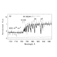
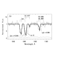
Figure 3$a$–$b$.— The normalized FOS/HST spectrum (histogram) and the tuned model predictions (not fits). The ticks mark locations of the constraint transitions identified for systems A, B, and C. Three models are shown. The thick solid spectrum includes the photoionized Mgii clouds, the photoionized diffuse component for systems B and C, and the photo plus collisionally ionized diffuse component for system A. The narrow solid spectrum includes the Mgii clouds and the photoionized diffuse components for each system. The dotted–line model includes the Mgii clouds only and is shown to illustrate the required high ionization phases. —($a$) The Lyman break and Lyman series. See text regarding the continuum fit, which is probably low in the region of 1760 Å to 1820 Å. Note the Nii $\lambda 916$ in system B and the Svi $\lambda\lambda 933,944$ in systems A and B. —($b$) The Ly$\gamma$, Ciii $\lambda 977$ and Niii $\lambda 989$ predictions. Note the sensitivity of Ciii to the model components.

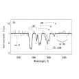
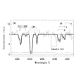
Figure 3$c$–$d$.— Same as Figure 3$a$ and 3$b$. —($c$) The Ly$\beta$, Ovi $\lambda\lambda 1031,1037$, and Cii $\lambda 1036$ predictions. The wavelength calibration may be shifted blueward in the region $\sim 1980$ to 2005 Å. Virtually no Ovi resides in the Mgii clouds, but must arise in a higher ionization phase. —($d$) The Siiii $\lambda 1206$, Ly$\alpha$, and Nv $\lambda\lambda 1238,1242$ predictions. Note the sensitivity of Ly$\alpha$ and Nv to the model components. The Siiii arises primarily in the Mgii clouds.

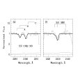
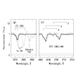
Figure 3$e$–$f$.— Same as Figure 3$a$ and 3$b$. —($e$) The Siii $\lambda\lambda 1190,1193$ doublet. The Siii also arises primarily in the Mgii clouds. —($f$) The Siii $\lambda 1260$ prediction. A blend (Ly$\alpha$?) must be present in the red wing. —($g$) The Cii $\lambda 1334$ prediction. As with Siii and Siiii, the Cii arises primarily in the Mgii clouds. Note the strong blend (Ly$\alpha$?) in the red wing. —($h$) The Siiv $\lambda\lambda 1393,1402$ doublet predictions. Since the Siiv also arises primarily in the Mgii clouds, the Siii, Siiii and Siiv ratios placed tight constraints on the cloud ionization conditions.

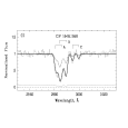
Figure 3$i$.— Same as Figure 3$a$ and 3$b$. The (self–blending) Civ $\lambda\lambda 1548,1550$ doublet predictions. For systems A and B, note that a fair fraction of the Civ arises in the Mgii clouds, but the majority must arise in a higher ionization phase.

Model clouds are drawn from the grid and a synthetic FOS spectrum is generated from the model column densities for the transitions listed in Table 2 (end of paper). The simulated FOS spectrum is generated by modeling the absorption from each transition by Voigt profiles convolved with the FOS instrumental spread function. The Doppler parameters of the modeled transitions are determined from the observed Mgii $b$ parameters and the kinetic temperature, $T$, output by the CLOUDY models, typically 5000 to 30,000 K. The CLOUDY temperature is used to estimate the thermal component of $b({\hbox{{\rm Mg}\kern 1.00006pt{\sc ii}}})$, from which the turbulent $b$ parameter is computed from the relation, $b_{tot}^{2}=b_{thermal}^{2}+b_{turb}^{2}$. The total $b$ parameter of any transition can then be estimated from its CLOUDY thermal $b$ and the turbulent $b$. The synthetic spectrum is then superimposed on the observed FOS spectrum and the $\chi^{2}$ is calculated pixel by pixel in regions of interest as an indicator of the goodness of the model.

3.2. High Ionization Gas

As will be shown, the model Mgii clouds could not account for even a small fraction of the absorption strengths of the higher ionization species (i.e. Civ, Svi, Nv, and Ovi). Thus, we postulated a high ionization diffuse component not seen in Mgii absorption. A maximal diffuse scenario provides the low ionization limit of the Mgii clouds such that their contribution to the moderate and high ionization species is minimized. A minimal diffuse scenario provides the high ionization limit of the Mgii clouds such that their contribution to the moderate and high ionization species is maximized.

For a postulated high ionization component, we used Civ and Ovi to constrain model cloud properties for both a solar abundance pattern, $\hbox{[C/O]}=0$, and an oxygen to carbon enhancement of $\hbox{[C/O]}=-0.5$. For constraints on the models from Svi, we use $[{\rm S}/{\rm H}]=0$, but note that sulfur is enhanced by $\sim 0.5$ dex for $[{\rm Fe}/{\rm H}]<0$. We avoid using Nv as a primary constraint because the chemical enrichment processes for nitrogen can lead to wide variations in its abundance (Wheeler, Sneden, & Truran (1989)). We adopt $\hbox{[N/O]}=0$ for this work, but occasionally discuss possible variations in this ratio.

To examine the range of properties of a diffuse component, we did the following systematic explorations. For each system, we first assumed that any required high ionization gas is in a single, broad component. The adopted models of the high ionization components are obtained using the same techniques illustrated in Appendix A, but the primary constraints are the residual strengths of the Civ and Ovi absorption unaccounted by the Mgii clouds. Also, consistency with any unaccounted Ciii, Siiii, Siiv, Svi and Nv is required. We then explored the possibility that the Civ arises in a few “Civ–only” clouds while the Ovi arises in a diffuse low density high ionization phase that is separate from the Civ clouds, which are separate from the Mgii clouds. The Nv and Svi absorption profiles were critical for constraining these “Civ cloud” models.

We systematically explored if contributions from both photoionization and collisional ionization are consistent with the data. For collisional ionization, we have drawn from the equilibrium models of Sutherland & Dopita (1993), with solar abundances. In these models, the relative column densities of various species, including that of neutral hydrogen, are a unique function of temperature for a given metallicity. Thus, under the model assumptions, the remaining free parameter is the temperature. To do so, we located the lowest ionization level of a photoionized diffuse component consistent with the intermediate and moderately high ionization species, after taking into account the Mgii clouds. A collisional ionization model was then tuned to any unaccounted absorption in Nv and Ovi.

4. Model Results

Our intent is to present a general picture of both the Mgii cloud and high ionization diffuse component properties within the context of our modeling. The adopted model properties are presented in Tables The Multiple Phases of Interstellar and Halo Gas in a Possible Group of Galaxies at $z\sim 1$, The Multiple Phases of Interstellar and Halo Gas in a Possible Group of Galaxies at $z\sim 1$, and 5. In Table The Multiple Phases of Interstellar and Halo Gas in a Possible Group of Galaxies at $z\sim 1$, we list the physical parameters of the twelve Mgii clouds for the scenarios of a maximal or minimal diffuse component. Typical model parameters for each system are given in Table The Multiple Phases of Interstellar and Halo Gas in a Possible Group of Galaxies at $z\sim 1$. The tabulated values serve as a guide; in the following discussion we quote allowed ranges in the cloud properties based upon § 3. The diffuse component properties are listed in Table 5. The results described below are for the Haardt & Madau (1996) extragalactic background. In Appendix B, we describe our explorations with several galactic/starburst radiation fields (representing both somewhat extreme and “normal” cases) and argue that our general conclusions are not altered. In Figure 3, we present the synthetic spectrum of our models superimposed upon the FOS spectrum. The model transitions are labeled with three–point ticks, which give the locations of systems A, B and C, from blue to red, respectively. Three synthetic spectra are shown. The dotted–line spectrum is of the twelve photoionized Mgii clouds. The thin solid–line spectrum includes both the Mgii clouds and the single–phase photoionized diffuse components. The thick solid–line spectrum includes a two–phase photo plus collisionally ionized component in system A.

4.1. System A $(z=0.9254)$

Since $N({\hbox{{\rm Fe}\kern 1.00006pt{\sc ii}}})/N({\hbox{{\rm Mg}\kern 1.00006pt{\sc ii}}})$ was not measured in any of the system A clouds, the clouds were assumed identical vis–á–vis their $N({\hbox{{\rm Mg}\kern 1.00006pt{\sc ii}}})$. The Siii to Siiv ratio tightly constrains the ionization level of these six clouds. There is only a very small range of allowed ionization conditions, with $\log U\simeq-2.3$. To avoid super solar metallicity, the mean $[\alpha/{\rm Fe}]$ ranges from $+0.3$ to $+0.5$, which corresponds to $0.0\leq Z\leq-0.2$, respectively, for the best match to the Lyman series. We obtained $10^{14.9}\leq N({\hbox{{\rm H}\kern 1.00006pt{\sc i}}})\leq 10^{15.6}$ cm^-2 in each of the six clouds; system A makes a negligible contribution to the Lyman limit break.

A highly ionized phase, not seen in Mgii, is required to account for the observed Civ, Nv, and Ovi absorption. For a single component, a Doppler width of $50\leq b\leq 100$ km s^-1 is consistent with the data. We ran a series of simulations, focused on the blended Civ profile, to explore the best combination of Doppler widths for Civ and Ovi in systems A and B, and to determine the allowed ranges for fits with with $\chi^{2}_{\nu}\leq 2$. Based upon these simulations, we adopted $b=70$ km s^-1. This component is consistent with either a single–phase photoionized diffuse medium with $\log U\simeq-1.2$, or a two–phase photo plus collisionally ionized diffuse medium with $\log U\simeq-1.26$ and $T\simeq 3\times 10^{5}$ K, respectively. All phases must be metal rich, $Z\sim 0$, in order to not overproduce the Lyman series. It is not possible to establish which of the two provides a better description of the high ionization transitions. The latter yields a better match to the Nv absorption. However, $[{\rm N}/{\rm O}]\simeq+0.15$ in the photoionized only phase could alternatively explain the Nv absorption. If the collisional component is present, further tests showed that Civ arising in a few clouds with smaller $b$ parameters was not ruled out. The bottom line is that a highly ionized phase is required, whether the Civ arises in a single or multiple clouds and the Ovi and Nv in a collisionally ionized phase, or whether the Civ, Nv, and Ovi all arise in a single highly photoionized phase.

For the photoionization scenario, the diffuse cloud size increased as $b$ was decreased from $70$ km s^-1, primarily due to the curve of growth behavior of Civ; its column density increases rapidly with decreasing $b$ and is effectively constant for $b>70$ km s^-1 in the relevant range of equivalent width. Based upon exploration of the allowed range of $b$ parameters, an upper limit on the size of the diffuse component is $\sim 30$ kpc for $b=50$ km s^-1. However, the best models, incorporating both a $\chi^{2}_{\nu}$ fit to the Civ profile and matching to the Nv, Svi, and Ovi profiles, had $b\geq 65$ km s^-1, which yielded sizes of $\sim 10$–$20$ kpc.

dummy space.

dummy space.

4.2. System B $(z=0.9276)$

A range of ionization conditions ($-3.2\leq\log U\leq-2.7$) for the clouds are found for this system, primarily based upon the observed Feii to Mgii ratios in clouds 8, 9, and 11, and upon Siii, Siiv and the other low ionization species for clouds 7 and 10. However, the low ionization limits (maximal diffuse scenario) are ruled out because the Siiv, Niii, and a large fraction of the Ciii must arise in the Mgii clouds. The Lyman limit break is primarily produced by clouds 8 and 11. For these clouds, the metallicity must be $Z\geq-0.2$, even for an $\alpha$–group enhanced abundance pattern, or else the Lyman limit break would be too large. In clouds 7 and 10, the allowed abundance pattern range is $0.0\leq[\alpha/{\rm Fe}]\leq+0.5$, corresponding to $-0.1\geq Z\geq-0.6$ (the lower limit is constrained by the Lyman series). The Siiv arises primarily in cloud 10, the most highly ionized, lowest density, and extended ($\sim 5$ kpc) Mgii cloud of the five. Even for the minimal diffuse scenario (high ionization limit), the predicted Civ absorption is still well below the observed strength.

Thus, an additional high ionization component, not seen in Mgii absorption, is required to account for the Civ, Nv, and Ovi absorption. This component is consistent with a single–phase photoionized diffuse medium ($b\simeq 70$ km s^-1, based upon the simulations of the Civ profile) with a solar abundance pattern and near solar metallicity. The bulk of the Civ, Nv, and Ovi absorption arises in this component, whereas the Niii and Siiv absorption arise primarily in cloud 10. The Ciii arises in both the Mgii clouds and the diffuse component. In Figure 3$a$, we point out the Nii $\lambda 916$ absorption, which accounts for the reduced flux in the Lyman break. We also point out the weak Svi $\lambda\lambda 933,944$ absorption, which arises in the diffuse component (the $\lambda 933$ transition is blended with Ly$6$ from system C). It is not possible for a collisionally ionized phase to substantially contribute.

As with system A, we obtained a maximum line of sight size, $S$, of $30$ kpc for the highly ionized diffuse component, but found a preferred size range of $10$–$20$ kpc. For $b\leq 50$ km s^-1, the larger cloud size elevated absorption in all high ionization species such that, in particular, Svi was significantly overproduced. A reduced $[{\rm S}/{\rm H}]$ would yield reduced sulfur absorption, but is unlikely because sulfur is usually enhanced relative to solar and is known to not suffer dust depletion (Lauroesch et al. (1996)).

4.3. System C $(z=0.9343)$

Though system C is a single weak Mgii cloud, it is best described by two photoionized phases. This inference is based upon a self–consistent match to the Lyman series, which is obtained when both a narrow and a broad component are included. The narrower low ionization Mgii cloud accounts for the Hi in the Ly$\gamma$, Ly$\delta$, and Ly$\epsilon$ absorption, whereas the broader high ionization diffuse component contributes significantly to the Ly$\alpha$ and Ly$\beta$ profiles.

The lower ionization phase produces the narrow Mgii, Siiii, and Siiv in a smaller cloud. We obtained $\log U\simeq-2.6$ and the range $-1.0\geq Z\geq-1.5$ for $0.0\leq[\alpha/{\rm Fe}]\leq+0.5$. The higher ionization phase, with $\log U\simeq-1.3$, has $b\sim 40$ km s^-1, which yields a size $S\sim 10$ kpc. It is not possible for this high ionization component to be strictly collisionally ionized nor is it possible for it to be a two–phase photo plus collisionally ionized component; any contribution from a collisionally ionized phase is insignificant.

5. Discussion

As shown in Figure 2, system A is comprised of six distinct Mgii clouds with a total velocity spread of $\sim 200$ km s^-1 and is $\sim-300$ km s^-1 from system B, which has five clouds spread over $\sim 100$ km s^-1. System C is $\sim+1000$ km s^-1 from system B and is comprised of a single, resolved Mgii cloud. In Figure 3, we show the normalized FOS spectrum with simulated spectra superimposed. These low resolution data reveal that each system is rich in multiple chemical species covering a wide range of ionization potentials and that the chemical and ionization conditions differ from system to system.

One motivation for our study was simply to ascertain if a multiphase medium was required to explain the strong Civ, Nv and Ovi absorption lines. In all three systems, we were required to postulate a higher ionization component that is not seen in Mgii absorption. We emphasize that (1) the overall Mgii cloud properties are well constrained by the data and modeling, and (2) the allowed cloud to cloud variations are constrained tightly enough that no scenario even remotely modifies the requirement for a Civ–Nv–Ovi high ionization phase to explain the data. To the accuracy afforded by the FOS spectrum, each of these high ionization phases is well described by a single component with $b\sim 70$ km s^-1 (based upon simulations). Given the large $b$ parameters and the range of sizes derived from the models (Table 5), this high ionization gas is likely to have a line of sight extent of $10\leq S\leq 20$ kpc, and thus may be a surrounding medium in which the $\sim 0.1$ kpc Mgii clouds are embedded.

5.1. Comparison of System Properties

Consider the cloud to cloud variations in system B, which is a Lyman limit system. The line of sight velocity spread of the Mgii clouds is $\sim 100$ km s^-1, which implies they are bound within a galactic potential. If the clouds are equally illuminated by the extragalactic background, then the presence of Feii in three of the clouds (8, 9, and 11) implies that they are more dense, more shielded from the ionizing flux, and/or iron–group enriched relative to the other two clouds (7 and 10). This suggests that clouds 8, 9, and 11 may be spatially contiguous (relatively speaking), in that they may share similar histories of iron–group enrichment from Type Ia SNe. In the Galaxy, the association of Type Ia explosions with the kinematically old disk implies that some events take place at large scale heights, so there is uncertainty in how much iron–rich gas is driven into galactic halos (Wheeler, Sneden, & Truran (1989)).

The unique cloud in system B is cloud 10, which gives rise to a broader absorption profile ($b\simeq 13$ km s^-1) and has no detectable Feii. It has a higher ionization condition and gives rise to the majority of the Siiv absorption (see Figure 4). It also has the largest $N({\hbox{{\rm Mg}\kern 1.00006pt{\sc ii}}})$. Models yield that it is extended ($\sim 5$ kpc) and has lower metallicity. This leads us to conservatively speculate that cloud 10 is more akin to a halo–like cloud or to a so–called Galactic high velocity cloud. The ratio $N({\hbox{{\rm Si}\kern 1.00006pt{\sc iv}}})/N({\hbox{{\rm Mg}\kern 1.00006pt{\sc ii}}})$ may be a useful indicator of the differing local environments of clouds in higher redshift systems.

System C classifies as a “weak” Mgii absorbers, defined by $W_{\rm r}(2796)<0.3$ Å (Churchill et al. 1999a ). From a sample of thirty such systems over the redshift range $0.4<z<1.4$, Churchill et al. found a wide range of $W_{\rm r}({\hbox{{\rm Fe}\kern 1.00006pt{\sc ii}}})/W_{\rm r}({\hbox{{\rm Mg}\kern 1.00006pt{\sc ii}}})$ and $W_{\rm r}({\hbox{{\rm C}\kern 1.00006pt{\sc iv}}})/W_{\rm r}({\hbox{{\rm Mg}\kern 1.00006pt{\sc ii}}})$, presumedly due to variations in abundance pattern and ionization conditions, including single phase and multiphase. These Mgii absorbers are sub–Lyman limit systems with $Z\geq-1$ and [some with $Z>0$ (Churchill & Le Brun (1998))]. Apart from its line–of–sight proximity ($<500$ km s^-1) to system B, system A would classify as a weak Mgii absorber. The $\sim 200$ km s^-1 kinematic spread of the six clouds in system A, and the large $N({\hbox{{\rm C}\kern 1.00006pt{\sc iv}}})/N({\hbox{{\rm Si}\kern 1.00006pt{\sc iv}}})$ ratio in the diffuse component are suggestive of lower ionization clouds moving within a high ionization galactic corona, or halo, where the ratio $N({\hbox{{\rm C}\kern 1.00006pt{\sc iv}}})/N({\hbox{{\rm Si}\kern 1.00006pt{\sc iv}}})$ is expected to be large (Savage et al. (1997)). Is it possible that the system C Mgii cloud arises in a similar environment as the six system A clouds, but that the line of sight happens to sample only one cloud? If so, the Civ absorption strength in system C would be comparable to that of system A, and it is significantly weaker. For weak systems, it may be that strong, broad Civ absorption implies a larger number of Mgii clouds with a larger kinematic spread.

5.2. Profile Anatomy: Model Predictions

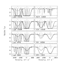
Figure 4.— A selection of predicted high resolution profiles for systems A and B based upon our models. This simulated STIS/HST spectrum has $R=30,000$ ($v\sim 10$ km s^-1) and signal–to–noise ratio of 30. Short ticks mark the velocities based upon the HIRES Mgii clouds and long ticks mark the diffuse component centroids. For system A, the three–phase model (photoionized Mgii clouds and photo plus collisionally ionized diffuse component) is shown and, for system B, the two–phase model (photoionized clouds and diffuse component) is shown. The dotted–line curves are the profiles of the blended individual Mgii clouds. The solid–line curves are the photoionized diffuse component profiles and the dash–dot curves are of the collisionally ionized diffuse component.

In Figure 4, we present simulated STIS/HST spectra with $R=30,000$, two pixels per resolution element, and a signal–to–noise ratio of $30$ for the first four transitions in the Lyman series, and for the Siiv, Civ, Nv, and Ovi profiles of systems A and B. These spectra were generated assuming Voigt profiles with the properties listed in Tables The Multiple Phases of Interstellar and Halo Gas in a Possible Group of Galaxies at $z\sim 1$ and 5. These model profiles can be compared directly to observed data (from STIS/HST) and thus provide a direct test of the models. We show the contributing components as smooth curves. The dotted–line curves are the Mgii clouds, with their velocity centroids marked with the short ticks above the continuum. The solid curves are from the photoionized diffuse component and the dash–dot curves in system A represents the collisionally ionized diffuse component.

5.2.1 The Lyman Series

Here, we emphasize the importance of the Lyman series. For all three systems, the Ly$\alpha$ and Ly$\beta$ profiles in the FOS spectra were significantly broader than could be fully accounted by the Hi obtained soley from the model Mgii clouds. However, the narrower Ly$\gamma$, Ly$\delta$, and Ly$\epsilon$ profiles were fully accounted by the Hi in these clouds. Based upon the curve of growth behavior of the Lyman series, we found that the addition of a very broad ($b>50$ km s^-1), lower $N({\hbox{{\rm H}\kern 1.00006pt{\sc i}}})$ component naturally explained the deeper and broader Ly$\alpha$ and Ly$\beta$ profiles, without overproducing the narrower Ly$\gamma$, Ly$\delta$, and Ly$\epsilon$ profiles (or modifying the Lyman limit break).

Such behavior of the Lyman series in low resolution data is likely to be a strong indication that a broad, perhaps highly ionized diffuse component is present. In Figure 4, we illustrate this behavior as it would be seen in higher resolution spectra. Note that the widths of Ly$\alpha$ and Ly$\beta$ are dominated by a broad, high ionization component, whereas the higher order transition widths are dominated by the Mgii clouds. In high resolution spectra, a diffuse component gives rise to a broadened, shallow wing when the profiles are saturated (see Ly$\alpha$ and Ly$\beta$ in system B) and/or suppresses the recovery of the flux to the continuum level between clouds in the profile centers (see Ly$\beta$ and Ly$\gamma$ in system A).

5.2.2 High Resolution Metal Lines

In system A, the Civ profiles have structure due to the lower ionization Mgii clouds. The Siiv absorption predominantly arises in the Mgii clouds, and thus closely traces the Mgii kinematics. Together, these profiles are tantalizing similar to those observed by Savage, Sembach, & Cardelli (1994) along the line of sight to HD 167756 in the Galaxy. We quote, “The sight line contains at least two types of highly ionized gas. One type gives rise to a broad Nv profile, and the other results in a more structured Siiv profile. The Civ profile contains contributions from both types of highly ionized gas.” We also find similarities between the model Civ profiles and those in the damped Ly$\alpha$ systems at $z_{\rm abs}=3.3901$ toward Q$0000-262$ and $z_{\rm abs}=2.2931$ toward Q$0216+080$ (Lu et al. 1996, Figures 2 and 3).

In system B, cloud 10 is clearly unique among the Mgii clouds. This cloud has the largest ionization parameter and accounts for the majority of the Siiv absorption, which was clearly constrained to arise in the Mgii clouds. Since the ionization conditions of clouds 8, 9, and 11 were set by their measured $N({\hbox{{\rm Fe}\kern 1.00006pt{\sc ii}}})/N({\hbox{{\rm Mg}\kern 1.00006pt{\sc ii}}})$, the ionization condition in cloud 10 was well constrained by the ratio $N({\hbox{{\rm Si}\kern 1.00006pt{\sc ii}}})/N({\hbox{{\rm Si}\kern 1.00006pt{\sc iv}}})$; there was no alternative but for cloud 10 to dominate the Siiv absorption. The point is that this cloud may arise in a spatially distinct environment and have a unique formation history from the other clouds in system B (see § 5). The Civ profile is dominated by a diffuse higher ionization phase, whereas the Siiv is predominantly due to higher density clouds. Some lines of sight through the Galaxy also exhibit narrow Siiv profiles and broad Civ profiles (for examples, see Sembach, Savage, & Jenkins (1994); Savage & Sembach (1994)). In contrast, the Siiv and Civ profiles in the $z_{\rm abs}=2.8268$ damped Ly$\alpha$ system towards Q$1425+603$ (Lu et al. (1996)) appear to arise in the same phase.

A synthetic STIS/HST spectrum for System C (not shown) reveals a narrow Siiv profile and broad Civ, Nv, and Ovi profiles. The Civ profile exhibits a slightly deep, narrow core due to the low ionization phase. However this contribution would be lost for the expected noise levels in observed data, unless this narrow component was off–center by $\sim 40$ km s^-1 relative to the broad component (within the uncertainty of our modeling such an offset is not ruled out).

6. On the Nature of the High Ionization Phase

Within 100″ of the QSO, Kirhakos et al. (1994) identified $10$ galaxies with $21\leq g\leq 22$. Compared to field galaxies, this is a slight overdensity by a factor of a few to several (Tyson (1988)). Identified within 10″ of the QSO are three bright galaxies with impact parameters $29$, $45$, and $47~{}h^{-1}$ kpc, respectively ($q_{0}=0.05$). At $z=0.93$, Thimm (1995) detected a [Oii] $\lambda 3727$ flux of $9\times 10^{-17}$ ergs cm^-2 s^-1 from the galaxy at $45~{}h^{-1}$ kpc.

Given these facts, we entertain the possibility that the Mgii absorption systems arise in individual galaxies either in a small group or possibly in a cluster. Such a possibility would have interesting implications in view of the types of mechanisms that could give rise to highly ionized gas in such environments.

6.1. Intragroup Corona?

Mulchaey et al. (1996) predicted that poor groups that are rich in spiral galaxies have hot, diffuse coronae that are cooler than the X–ray coronae surrounding poor groups dominated by E/S0 galaxies. This high ionization intragroup material is predicted to have $T\sim 2\times 10^{6}$ K and to primarily give rise to strong Ovi, whereas any Civ or Nv absorption is predicted to arise in the proximity of the galaxies themselves (Mulchaey et al. (1996)). As such, the Ovi profiles would be broader than the Nv and Civ. The same would hold for the Lyman series (Verner, Tytler, & Barthel (1994)).

Our models can fully explain the Ovi, Nv, and Civ in a single component of $T\sim 3\times 10^{4}$ K gas (the possible collisional component in system A has $T\sim 3\times 10^{5}$ K). The observed Ovi or Hi widths are not broader than those of the Civ and Nv, and their $\sim 70$ km s^-1 $b$ parameters are not suggestive of gas that is kinematically akin to the $\sim 200$ km s^-1 dispersion of a galaxy group. Furthermore, the Ovi, Nv, and Civ profiles are clearly aligned with the three Mgii absorption redshifts, suggesting that the high ionization material is spatially coincident with the individual Mgii systems. The upper limit on the size of the photoionized diffuse components is $S\leq 30$ kpc (assuming photoionization equilibrium), and the inferred $Z\sim 0$ metallicities suggest that the high ionization material surrounds the galaxies and has been enriched by them. Significantly lower metallicities are expected if the gas was intragroup material left over from the formation processes. We do not favor an interpretation of the data in which the high ionization material arises in a intragroup or common halo.

6.2. Galactic Coronae?

The highly ionized material in these three $z\sim 1$ galaxies may be more akin to galactic coronae (see Spitzer 1956, 1990; Savage et al. 1997), material stirred up by energetic mechanical processes, such as galactic fountains. In this scenario, the gas is concentrated around individual galaxies which presumably provide a source of support, heating, and chemical enrichment.

In the Galaxy, $b\simeq 60$ km s^-1 was measured for Civ, and was observed to slightly increase with the ionization level of the transition (Savage et al. (1997)). Simulations of the allowed range of $b$ parameters for systems A and B yielded similar Doppler widths, with $b\simeq 70$ km s^-1 providing a good match to the Civ, Nv, and Ovi profiles for both systems. If the high ionization diffuse components in these systems are arising in coronae analogous to that surrounding the Galaxy, they may have similar turbulent processes supporting their scale heights.

The radial extent of the Galactic corona is unknown, but for local galaxies, radio maps reveal Hi extends to tens of kpc (Corbelli, Schneider, & Salpeter (1989); van Gorkom et al. (1993)), beyond which the hydrogen becomes optically thin and a highly ionized extension is expected (Maloney (1993); Corbelli & Salpeter (1993); Dove & Shull (1994)). The impact parameters of the candidate galaxies are $\sim 30$–$50~{}h^{-1}$ kpc, with the orientation of the line of sight through each galaxy unknown. Absorption, even from non–spherical absorbers, is not unexpected at an impact parameter of $\sim 50$ kpc (see Figure 1 of Charlton & Churchill (1996)). For the Galaxy, Savage et al. (1997) measured the effective scale heights of $5.1$, $4.4$, and $3.9$ kpc for Siiv, Civ, and Nv, respectively. We find a preferred size of $10$–$20$ kpc for the size of the high ionization gas at $z\sim 0.93$, with an upper limit of $\sim 30$ kpc. Since these “sizes” (or the path length through an oriented structure) are comparable to twice the Galactic scale height, the distribution of high ionization is consistent with Galactic–like coronae.

A scenario in which the high ionization gas arises in individual galactic coronae is in contrast to that proposed by Lopez et al. (1998) for a system at $z\sim 1.7$ in the spectra of HE $1104-181$ A, B. In a double line of sight study, Lopez et al. found Ovi profiles consistent with $110\leq b\leq 180$ km s^-1 and that the extent of the highly ionized gas was $\sim 100$ kpc. These inferences also differ from those of Bergeron et al. (1994), who found that the Ovi phase in the $z_{\rm abs}\sim 0.8$ Mgii absorber toward PKS $2145+064$ was at least $50$ kpc in extent.

7. Conclusions

We have studied the kinematic, chemical, and ionization conditions of three metal–line absorption systems at $z\sim 1$ seen in the PG $1206+459$ spectrum. The systems were selected by the presence of Mgii absorption in a high resolution spectrum, and were chosen as a pilot study of a larger program designed to chart the physical conditions and evolution of absorbing gas in galaxies. The Mgii profiles are shown in Figure 1, with each system designated A, B, and C. Rich absorption line data from FOS/HST (Jannuzi et al. (1998)) revealed strong Civ, Nv, and Ovi absorption, as well as Hi and many other species and transitions covering a wide range of ionization potentials. Ground–based imaging data (Kirhakos et al. (1994)) revealed three candidate absorbing galaxies within 10″ of the QSO and possibly a group of galaxies within 100″ of the QSO.

The main goals of the study were to see if multiphase gas was required to explain the strong high ionization absorption line data, and to infer some level of information on the gas metallicities and spatial distributions. Assuming the Mgii clouds are photoionized, we found the range of chemical and ionization conditions consistent with both the high resolution and low resolution data. We then postulated the presence of high ionization components not seen in Mgii absorption to explain the unaccounted Ciii, Civ, Nv, and Ovi absorption.

We briefly summarize the main results of our study:

1. For systems A and B, we were required to postulate a high ionization phase in addition to the lower ionization Mgii clouds. System C could be made marginally consistent with a single–phase absorber, though a two–phase absorber is strongly preferred due to the nature of the Lyman series absorption. We infer that, in these systems, the lower ionization Mgii clouds arise in high ionization diffuse gas; each of these absorption systems is comprised of a multiphase gaseous medium. We find that the high ionization phase of system A could arise in multiple, narrower “Civ clouds”. For system B, such Civ clouds are ruled out.

2. The absorbing gas in both the Mgii clouds and the high ionization components are consistent with photoionized clouds. In systems B and C, a collisionally ionized phase is ruled out. Only in system A could the data be made consistent with a three–phase absorber, incorporating the photoionized Mgii clouds, a highly photoionized diffuse component, and a collisionally ionized component. This three–phase model provided a more consistent match to the Nv absorption in this system. In this three–phase scenario, the Civ could arise in a few narrower components. However, $[{\rm N}/{\rm O}]\simeq 0.15$ in the highly photoionized component, instead of the assumed $[{\rm N}/{\rm O}]=0$, would remove the need for the collisionally ionized gas and rule out the three–phase absorber.

3. We find no evidence that the Ovi gas is in a separate and very highly ionized diffuse phase that encompasses the Civ and Nv absorption. Based upon the $b\sim 70$ km s^-1 profile widths, inferred $Z\sim 0$ metallicities, $3\times 10^{4}$ K temperatures, inferred $S\leq 30$ kpc sizes, and the clear redshift alignment of the high ionization transitions with the Mgii systems, we suggest that the high ionization gas is analogous to the Galactic corona in that it traces the galaxies themselves and does not appear to exhibit the characteristics predicted for intragroup or intracluster material. The Ovi likely arises in the same phase as the Civ and Nv. The Siiv is constrained to arise in the same phase as the Mgii clouds, whereas Ciii arises in both the clouds and the high ionization phase.

4. We have found cloud to cloud variations in the chemical and ionization conditions in the five Mgii clouds of system B. Three of the clouds are likely to be iron–group enriched and have higher densities and low ionization conditions. The majority of the neutral hydrogen giving rise to the Lyman break in the FOS spectrum is from these clouds. A lower metallicity Mgii cloud giving rise to a broader absorption profile is interspersed in velocity with these clouds, likely has an $\alpha$–group enhanced abundance pattern, and gives rise to the majority of the Siiv absorption. We speculate that this cloud may be similar to a halo–like cloud, and suggest that the ratio $N({\hbox{{\rm Si}\kern 1.00006pt{\sc iv}}})/({\hbox{{\rm Mg}\kern 1.00006pt{\sc ii}}})$ may be a useful indicator for discriminating between clouds in different parts of high redshift galaxies.

The most compelling reason why we favor the scenario in which the high ionization diffuse material is coupled to the galaxies is the clear kinematic separation of the Ovi profiles corresponding to systems A and B. Each of the inferred diffuse components must be centered (at least roughly) on the systems, and they must be distinct from one another in velocity space. There are additional, if less compelling, arguments. The inferred $b$ parameters in the model diffuse components are in the same regime as those found for the Galactic corona (Savage et al. (1997)), further suggesting that the material is galaxy associated. The inferred metallicities are high, $Z\sim 0$, which is best understood if the material had been enriched by its host galaxy and further suggests that the origin and source of enrichment of the diffuse gas is related to star forming parts of galaxies. The enrichment could be due to in situ star formation as gas clouds collide and cool in the galactic halos (Steidel & Sargent (1992)), or could be due to galactic fountain processes from the galactic disks (Spitzer (1990)).

As a speculative aside, we ask if Galactic–like coronae Ovi absorbers are likely to be a common form of Ovi systems at $z\leq 1$, as opposed to group–halos. Burles & Tytler (1996) have shown that absorbers selected by the presence of Ovi have the same redshift path density as Lyman limit–Mgii absorbers at $\left<z\right>=0.9$. As we have found here, Ovi can be associated with a Lyman limit system when the absorbing gas is segregated into multiple ionization phases. If multiphase absorption is common in Mgii absorbers, some Ovi might arise in Galactic–like corona.

It would seem that this pilot study has shown that wholesale study of the kinematic, chemical, and ionization conditions of Mgii absorbers, using high resolution Mgii profiles and the available low resolution HST spectra, would yield a improved understanding of galactic gas at early epochs. In order to assess the robustness of our modeling, we have synthesized high resolution STIS/HST spectra of the ultraviolet transitions (presented in Figure 4). The modeling techniques applied in this paper can be directly tested by comparing these predicted profiles with those observed with STIS/HST. If our approach proves to yield an accurate description of the gas, then wholesale modeling can be embarked upon for roughly 50 Mgii systems without requiring large amounts of space based telescope time to acquire high resolution spectra of high quality.

Appendix A Application of Observed Constraints

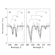
Figure A1.— An illustration of how the Siii $\lambda\lambda 1190,1193$ (panel $a$) and Siiv $\lambda\lambda 1393,1402$ (panel $b$) doublets were used to constrain the ionization conditions for the photoionized Mgii clouds in systems A, B, and C. The clouds are tuned by the ratio $f=\log\{N({\hbox{{\rm Fe}\kern 0.80005pt{\sc ii}}})/N({\hbox{{\rm Mg}\kern 0.80005pt{\sc ii}}})\}$, which yields a unique ionization parameter, $U$ (clouds with measured Feii are fixed). The dotted–line curve is for the $1\sigma$ limits on $f$ for each cloud as measured from the HIRES data. The solid, dash, and dot–dash curves are for $f=-3.0$, $-3.5$, and $-4.0$, respectively. The corresponding ionization parameters are $\log U=-2.30$, $-2.15$, and $-2.00$ (a small range, indeed). The ratio $N({\hbox{{\rm Si}\kern 0.80005pt{\sc ii}}})/N({\hbox{{\rm Si}\kern 0.80005pt{\sc iv}}})$ decreases with decreasing $f$, or equivalently, as the ionization parameter is increased.

In this appendix, we demonstrate our modeling methodology for constraining the ionization parameters, metallicities, and overall Mgii cloud properties using the FOS/HST data.

In Figure A1, we present an example of how the data are used to constrain the ionization parameter, $U$. In Figure A1$a$ the synthetic FOS spectrum of the Siii $\lambda\lambda 1190,1193$ doublet is superimposed on the FOS data for the $1\sigma$ upper limits on $\log\{N({\hbox{{\rm Fe}\kern 1.00006pt{\sc ii}}})/N({\hbox{{\rm Mg}\kern 1.00006pt{\sc ii}}})\}$, and for the set ratios $-3.0$, $-3.5$, and $-4.0$. The Siiv $\lambda\lambda 1393,1402$ doublet is shown in Figure A1$b$. The assumed abundance pattern is solar. Clouds 8, 9, and 11 have their $U$ constrained by the observed $\log\{N({\hbox{{\rm Fe}\kern 1.00006pt{\sc ii}}})/N({\hbox{{\rm Mg}\kern 1.00006pt{\sc ii}}})\}$. The ratio of Siii to Siiv can uniquely determine $U$ for the remaining clouds. For System A, the best match is provided by $\log U=-2.3$ [which corresponds to $\log\{N({\hbox{{\rm Fe}\kern 1.00006pt{\sc ii}}})/N({\hbox{{\rm Mg}\kern 1.00006pt{\sc ii}}})\}=-3.0$]. Lower ionization clouds are not possible because they overproduce Siii, whereas higher ionization clouds overproduce Siiv. For System B, a reasonable match to the observed Siii and Siiv is achieved if clouds 7 and 10 (dominated by 11 because of its larger Mgii column density) are assigned $\log U=-2.0$, which corresponds to $\log\{N({\hbox{{\rm Fe}\kern 1.00006pt{\sc ii}}})/N({\hbox{{\rm Mg}\kern 1.00006pt{\sc ii}}})\}=-4.0$. Less ionized clouds are possible, but an additional more highly ionized component would then be required to produce Siiv.

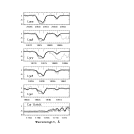
Figure A2.— An illustration of how the Lyman series was used for tuning the metallicity, $Z$, and neutral hydrogen column density, $N({\hbox{{\rm H}\kern 0.80005pt{\sc i}}})$, for set ionization conditions. Only the photoionized Mgii clouds are shown. For these clouds the ionization conditions were tightly constrained by the Siii, Siiii, and Siiv data. The ticks mark systems A, B, and C, from left to right. A solar abundance pattern is assumed. The thick solid model has $Z=0$ (solar); the dotted–line model with stronger $N({\hbox{{\rm H}\kern 0.80005pt{\sc i}}})$ absorption has $Z=-0.4$; and, the dotted–line model with the weaker absorption has $Z=+0.4$. Note that the series is not fit self–consistently for any value of $Z$ (see § 5.2).

In Figure A2, we present an example of how the Lyman series and limit are used to constrain the metallicity for the ionization parameters determined in the above illustration. We have assumed $\hbox{[$\alpha$/Fe]}=0$ for this illustration. Three metallicities are shown, $Z=-0.4$, $0.0$, and $+0.4$, to illustrate the strength variations in the Lyman series and limit. At low metallicity, a large $N({\hbox{{\rm H}\kern 1.00006pt{\sc i}}})$ is needed to produce the observed metal lines with low and intermediate ionization levels. Such a large $N({\hbox{{\rm H}\kern 1.00006pt{\sc i}}})$ can be inconsistent with the observed Lyman series lines and Lyman limit break. As described in § 2, the Lyman limit break implies a total $N({\hbox{{\rm H}\kern 1.00006pt{\sc i}}})$ of $10^{17.2}$ cm^-2. For System A, the best match to the Lyman series lines is given by $Z=+0.2$, super–solar metallicity. For System B, the best match also has high metallicity; clouds 8, 9, and 11 must have $Z=0.0$, and cloud 10 must also have near solar metallicity in order that there is not too large an $N({\hbox{{\rm H}\kern 1.00006pt{\sc i}}})$. It is important to point out that the assumed abundance pattern directly affects the inferred metallicities. If the abundance pattern is $\alpha$–group enhanced, $\hbox{[$\alpha$/Fe]}=+0.5$, the illustrated metallicities would proportionally drop by $\sim 0.5$ dex. This is because the cloud properties are tuned to the $N({\hbox{{\rm Mg}\kern 1.00006pt{\sc ii}}})$, and magnesium is an $\alpha$–group element (see § 3).

Appendix B Galactic Ionizing Photons?

Given the [Oii] $\lambda 3727$ emission measured by Thimm (1995), it is reasonable to assume that high energy photons could be escaping the galaxies (e.g. Bergeron et al. (1994)). The Thimm measurement of an [Oii] flux from one galaxy (and limits for the others) constrains the contribution of galactic ionizing photons to be $<7\times 10^{5}$ cm^-2 s^-1 under the assumption that 50% of the photons escape from the galaxy. This is a factor of five to 50 times greater than that estimated for the Galaxy (Bland–Hawthorn & Maloney (1999)) and for external galaxies (Deharveng et al. (1997)), respectively. Keeping this generous upper limit in mind, we consider the effect a change in spectral shape could have on our main results. Several contrasting starburst models from Bruzual & Charlot (1993) were explored. In all cases, the galaxy spectra were normalized relative to the Haardt & Madau (1996) flux, $F_{HM}$, at 1 Rydberg. Depending on the spectral shape, the above limit corresponds to $F_{sb}/F_{HM}<4$–$10$, where $F_{sb}$ is the flux of the starburst galaxy model at 1 Rydberg.

First we consider a $10^{7}$ year instantaneous burst model, because of its prominent Hei edge [see Fig. 4 of Bruzual & Charlot (1993)]. As the ratio $F_{sb}/F_{HM}$ is increased, the hydrogen becomes more ionized and it is possible to decrease the cloud metallicities without overproducing Hi. However, only a modest decrease of 0.4 dex is possible for $F_{sb}/F_{HM}\leq 10$. For these models, there are relatively fewer photons capable of ionizing Ciii and thus there is even less Civ produced in the Mgii clouds. Similarly, in order to maintain the observed Siii to Siiv ratio, it is necessary to slightly increase the cloud ionization parameter by a few tenths of a dex from the pure Haardt & Madau case. We also consider the effect of the change in spectral shape upon the diffuse phase that produces Civ and Ovi. Similar conclusions hold for the metallicity, which can decrease by at most 0.5 dex from the pure Haardt & Madau case; the diffuse phase still must have relatively high metallicity ($>0.3Z$). For energies greater than the Heii edge, this overall spectrum is unchanged relative to Haardt & Madau, and therefore the balance between Civ and Ovi, and other high ionization energy transitions is unaltered.

In order to explore a severe Hi edge, we explored another extreme model, a $10^{8}$ year instantaneous burst. In this case the measured [Oii] constraint also forces the upper limit $F_{sb}/F_{HM}\leq 10$. Interestingly, the Mgii cloud metallicity cannot be reduced (relative to pure Haardt & Madau) because $N({\hbox{{\rm H}\kern 1.00006pt{\sc i}}})$ actually increases relative to $N({\hbox{{\rm Mg}\kern 1.00006pt{\sc ii}}})$ as the galaxy contribution is increased. Due to similar behavior, the metallicity of the required diffuse component is constrained to be solar or super–solar. The change in spectral shape has the effect of increasing Siiv and Svi, but decreasing Ciii. The bulk of the Siiv still arises in the Mgii clouds, but Svi in the diffuse phase is overproduced, and the required super–solar metallicity seems implausible.

Finally, we consider a later–type galaxy model with a 16 Gyr stellar population and with exponentially decreasing but persistent, star formation [the $\mu=0.01$ model (Bruzual (1983))]. This model has 1% of the total star–forming mass in stars after 1 Gyr. The star formation longevity of this relatively quiescent galaxy is more plausible than an instantaneous burst. As the galactic flux is incrementally increased relative to the extragalactic background, the metallicity constraints are unchanged, but the ratio $N({\hbox{{\rm C}\kern 1.00006pt{\sc iv}}})/N({\hbox{{\rm Mg}\kern 1.00006pt{\sc ii}}})$ decreases due to the drop in flux at the Heii edge. Thus, the requirement for a diffuse component in these absorbers is strengthened if galactic flux is contributing. We also found that it is increasingly difficult to produce the required $N({\hbox{{\rm O}\kern 1.00006pt{\sc vi}}})/N({\hbox{{\rm C}\kern 1.00006pt{\sc iv}}})$ ratio as the galactic flux is increased unless the ionization parameter is significantly increased. This results in the destruction of Siiv. Thus, our conclusion that the Siiv must arise in the Mgii clouds is also strengthened if such a galactic flux is contributing to or dominating the ionizing spectrum. Likewise, our conclusion holds that any collisionally ionized diffuse component in system B must be negligible. As with the extragalactic background scenario, the Ciii becomes too large and inconsistent with the data if one lowers the ionization condition in the photoionized diffuse component.

Although some starburst galaxy spectra can somewhat decrease the constraint on the cloud and diffuse component metallicities, this effect is limited to less than 0.5 dex due to constraints on [Oii] emission. These galaxies are not strong starbursts, though they could have modest galaxy contribution to the spectral shape. Thus, we find that our general conclusions with regard to the requirement of highly ionized diffuse components and relatively high metallicity clouds are not sensitive to the assumed spectral shape of the ionizing flux, though the details of the adopted models would be somewhat modified.

Table 1HIRES/Keck Mgii and Feii Data

					Mgii			Feii
Sys	Cld	$z_{\rm abs}$	$v$		$\log N$	$b$		$\log N$	$b$	Feii/Mgii
	No.		[km s-1]		[cm-2]	[km s-1]		[cm-2]	[km s-1]	[$\log$]
A	1	0.92501	$-403.5$		$11.92\pm 0.03$	$5.98\pm 0.55$		$<11.47$	$\cdots$	$<-0.5$
A	2	0.92535	$-350.7$		$12.16\pm 0.02$	$2.89\pm 0.26$		$<11.48$	$\cdots$	$<-0.7$
A	3	0.92550	$-327.7$		$12.12\pm 0.02$	$2.98\pm 0.28$		$<11.48$	$\cdots$	$<-0.6$
A	4	0.92595	$-256.8$		$12.35\pm 0.01$	$4.77\pm 0.20$		$<11.48$	$\cdots$	$<-0.9$
A	5	0.92639	$-188.0$		$12.01\pm 0.02$	$3.10\pm 0.37$		$<11.49$	$\cdots$	$<-0.5$
A	6	0.92648	$-174.2$		$11.60\pm 0.05$	$3.69\pm 0.89$		$<11.49$	$\cdots$	$<-0.1$
B	7	0.92720	$-62.8$		$11.72\pm 0.07$	$16.19\pm 3.54$		$<11.47$	$\cdots$	$<-0.3$
B	8	0.92742	$-29.0$		$13.44\pm 0.04$	$5.67\pm 0.15$		$12.75\pm 0.02$	$6.19\pm 0.27$	$-0.7$
B	9	0.92764	$6.0$		$13.29\pm 0.01$	$7.38\pm 0.14$		$12.21\pm 0.06$	$8.52\pm 1.26$	$-1.1$
B	10	0.92780	$30.4$		$12.60\pm 0.01$	$12.70\pm 0.49$		$<11.45$	$\cdots$	$<-1.2$
B	11	0.92803	$66.0$		$12.82\pm 0.01$	$5.08\pm 0.10$		$12.07\pm 0.05$	$2.85\pm 0.76$	$-0.8$
C	12	0.93428	$1038.3$		$12.05\pm 0.02$	$7.52\pm 0.52$		$<11.41$	$\cdots$	$<-0.6$

Table 2FOS/HST Identified/Constraint Lines

No.	$\lambda$	Line ID		IP	Sys		Notes
	[Å]	Ion	$\lambda$, Å	[eV]
1a	1762.92	Nii	915.61	29.6	A
2a	1765.03	Nii	915.61		B		matches depression at Lyman limit
3a	1770.98	Nii	915.61		C
4a	1797.13	Svi	933.38	88.0	A		C-fit?
5a	1799.19	Svi	933.38		B		Bl–Ly$6$ from sys C; C–fit?; Note
6a	1805.42	Svi	933.38		C		Bl–7a; C-fit?
7a	1805.65	Ly$\epsilon$	937.80	13.6	A		Bl–6a; C-fit?
8a	1807.80	Ly$\epsilon$	937.80		B
9a	1813.90	Ly$\epsilon$	937.80		C
10a	1818.58	Svi	944.52	88.0	A
11a	1820.66	Svi	944.52		B
12a	1826.97	Svi	944.52		C		Bl–13a
13a	1828.64	Ly$\delta$	949.74	13.6	A		Bl–12a
14a	1830.82	Ly$\delta$	949.74		B
15a	1836.99	Ly$\delta$	949.74		C
16b	1872.52	Ly$\gamma$	972.54		A
17b	1874.76	Ly$\gamma$	972.54		B
18b	1881.08	Ly$\gamma$	972.54		C		Bl–19b; Bl–Ly$\alpha$
19b	1881.15	Ciii	977.02	47.9	A		Bl–18b
20b	1883.40	Ciii	977.02		B
21b	1889.75	Ciii	977.02		C
22b	1905.76	Niii	989.80	47.4	A		Bl–Ly$\alpha$ or Ly$\beta$?
23b	1908.04	Niii	989.80		B
24b	1914.47	Niii	989.80		C
25c	1974.93	Ly$\beta$	1025.72	13.6	A
26c	1977.28	Ly$\beta$	1025.72		B
27c	1983.95	Ly$\beta$	1025.72		C
28c	1986.87	Ovi	1031.93	138.1	A
29c	1989.25	Ovi	1031.93		B
30c	1995.36	Cii	1036.33	24.3	A		Bl–31c; Bl–Ly$\alpha$?
31c	1995.95	Ovi	1031.93	138.1	C		Bl–30c; Bl–Ly$\alpha$?
32c	1997.75	Cii	1036.34	24.3	B		Bl–33c
33c	1997.83	Ovi	1037.62	138.1	A		Bl–32c
34c	2000.21	Ovi	1037.62		B		Bl–Ly$\alpha$?
35c	2004.48	Cii	1036.34	24.3	C
36c	2006.96	Ovi	1037.62	138.1	C
37e	2292.03	Siii	1190.42	16.3	A
38e	2294.76	Siii	1190.42		B
39e	2297.56	Siii	1193.29		A
40e	2300.31	Siii	1193.29		B
41e	2302.50	Siii	1190.42		C
42e	2308.06	Siii	1193.29		C
43d	2323.00	Siiii	1206.50	33.5	A
44d	2325.77	Siiii	1206.50		B
45d	2333.61	Siiii	1206.50		C
46d	2340.65	Ly$\alpha$	1215.67	13.6	A
47d	2343.45	Ly$\alpha$	1215.67		B
48d	2351.35	Ly$\alpha$	1215.67		C
49d	2385.23	Nv	1238.82	97.9	A		Bl–Galactic Feii
50d	2388.08	Nv	1238.82		B
51d	2392.89	Nv	1242.80		A
52d	2395.75	Nv	1242.80		B		Bl–53d
53d	2396.13	Nv	1238.82		C		Bl–52d
54d	2403.83	Nv	1242.80		C
55f	2426.82	Siii	1260.42	16.3	A
56f	2429.72	Siii	1260.42		B		Bl–Ly$\alpha$?
57f	2437.91	Siii	1260.42		C
58g	2569.51	Cii	1334.53	24.4	A
59g	2572.58	Cii	1334.53		B		Bl–Ly$\alpha$?
60g	2581.25	Cii	1334.53		C		Bl–Ly$\alpha$?
61h	2683.54	Siiv	1393.76	45.1	A		Note
62h	2686.74	Siiv	1393.76		B
63h	2695.80	Siiv	1393.76		C
64h	2700.89	Siiv	1402.77		A
65h	2704.12	Siiv	1402.77		B
66h	2713.24	Siiv	1402.77		C
67i	2980.89	Civ	1548.20	64.5	A
68i	2984.46	Civ	1548.20		B		Bl–69i
69i	2985.85	Civ	1550.77		A		Bl–68i
70i	2989.42	Civ	1550.77		B
71i	2994.52	Civ	1548.20		C
72i	2999.50	Civ	1550.77		C

Note. — The letter component to the line number gives the Figure 3 panel designation. “C–fit?” indicates that the continuum fit is somewhat uncertain. “Bl–X” indicates an identified line blend.

[l] 3. Bracketed Ionization Conditions Maximal Diffuse Minimal Diffuse (Low Ionization Limits) (High Ionization Limits) Sys Cld $N({\hbox{{\rm Mg}\kern 1.00006pt{\sc ii}}})$ $U$ $Z$ Feii/Mgii $N({\hbox{{\rm H}\kern 1.00006pt{\sc i}}})$ $N({\hbox{{\rm C}\kern 1.00006pt{\sc iv}}})$ $S$ [pc] $U$ $Z$ Feii/Mgii $N({\hbox{{\rm H}\kern 1.00006pt{\sc i}}})$ $N({\hbox{{\rm C}\kern 1.00006pt{\sc iv}}})$ $S$ [pc] (1) (2) (3) (4) (5) (6) (1) (2) (3) (4) (5) (6) A^a 1 11.92 $-2.5$ $-0.2$ $-3.0$ $15.0$ $13.3$ $90$ $-2.5$ $-0.2$ $-3.0$ $15.0$ $13.3$ $90$ A 2 12.16 $-2.5$ $-0.2$ $-3.0$ $15.2$ $13.5$ $150$ $-2.5$ $-0.2$ $-3.0$ $15.2$ $13.5$ $150$ A 3 12.12 $-2.5$ $-0.2$ $-3.0$ $15.2$ $13.5$ $140$ $-2.5$ $-0.2$ $-3.0$ $15.2$ $13.5$ $140$ A 4 12.35 $-2.5$ $-0.2$ $-3.0$ $15.4$ $13.7$ $230$ $-2.5$ $-0.2$ $-3.0$ $15.4$ $13.7$ $230$ A 5 12.35 $-2.5$ $-0.2$ $-3.0$ $15.1$ $13.4$ $110$ $-2.5$ $-0.2$ $-3.0$ $15.1$ $13.4$ $110$ A 6 11.60 $-2.5$ $-0.2$ $-3.0$ $14.7$ $13.0$ $40$ $-2.5$ $-0.2$ $-3.0$ $14.7$ $13.0$ $40$ B 7 11.72 $-4.0$ $-0.6$ $-0.7$ $15.7$ $6.7$ $1$ $-2.2$ $-0.6$ $-4.0$ $15.4$ $13.8$ $780$ B^b 8 13.44 $-3.2$ $0.0$ $-0.7$ $16.7$ $13.2$ $110$ $-3.2$ $0.0$ $-0.7$ $16.7$ $13.2$ $110$ B^b 9 13.29 $-3.4$ $0.0$ $-1.1$ $16.5$ $13.6$ $210$ $-3.0$ $0.0$ $-1.1$ $16.5$ $13.6$ $210$ B 10 12.60 $-3.1$ $-0.6$ $-1.6$ $16.2$ $12.6$ $60$ $-2.3$ $-0.6$ $-4.0$ $16.0$ $14.6$ $5200$ B^b 11 12.82 $-3.2$ $0.0$ $-0.8$ $16.1$ $12.7$ $30$ $-3.2$ $0.0$ $-0.8$ $16.1$ $12.7$ $30$ C 12 12.05 $-3.1$ $-1.0$ $-1.1$ $16.3$ $12.3$ $100$ $-2.0$ $-0.4$ $-4.5$ $16.3$ $15.3$ $26000$ Note. — Systems A and B are $\alpha$–group enhanced by 0.5 dex, whereas System C has solar abundance ratios. Column 1 is the log of the ionization parameter (see text). The number density of hydrogen is given by $\log n_{H}=-(\log U+5.2)$. Column 2 is the metallicity, [$Z/Z_{\odot}$]. Column 3 is the ratio of the Feii and Mgii column densities, $\log N({\hbox{{\rm Fe}\kern 1.00006pt{\sc ii}}})-\log N({\hbox{{\rm Mg}\kern 1.00006pt{\sc ii}}})$. Columns 4 and 5 are the log of the Hi and Civ column densities in atoms cm^-2. Column 6 is the linear depth of the cloud in parsecs. ^a Note that the low and high ionization “limits” of system A are presented to be identical. In fact, the limits are very narrow due to the contraints provided by the Siii and Siiv profiles (see text). ^b The Feii/Mgii ratio of this cloud is fixed by measurement. The cloud abundance ratio pattern is assumed solar, not $\alpha$–group enhanced (see text).

[l] 4. Photoionized Mgii Cloud Properties Cloud Number Property IP 1 2 3 4 5 6 7 8 9 10 11 12 [eV] $z_{\rm abs}$ 0.92501 0.92535 0.92550 0.92595 0.92639 0.92648 0.92720 0.92742 0.92764 0.92780 0.92803 0.93428 $v$ $-403.5$ $-350.7$ $-327.6$ $-256.8$ $-187.9$ $-174.2$ $-62.8$ $-29.0$ $6.0$ $30.3$ $66.0$ $1039.3$ $\log U$ $-2.5$ $-2.5$ $-2.5$ $-2.5$ $-2.5$ $-2.5$ $-2.2$ $-3.2$ $-3.0$ $-2.2$ $-3.2$ $-2.6$ $S$ [pc] 90 150 140 230 110 40 780 110 210 5200 30 1700 $Z$ $-0.2$ $-0.2$ $-0.2$ $-0.2$ $-0.2$ $-0.2$ $-0.6$ $0.0$ $0.0$ $-0.6$ $0.0$ $-1.0$ $[\alpha/{\rm Fe}]$ $+0.5$ $+0.5$ $+0.5$ $+0.5$ $+0.5$ $+0.5$ $+0.5$ $0.0$ $0.0$ $+0.5$ $0.0$ $0.0$ $N({\hbox{{\rm H}\kern 1.00006pt{\sc i}}})$ 13.6 15.0 15.2 15.2 15.4 15.1 14.7 15.4 16.7 16.5 16.2 16.1 16.4 $N({\rm H})$  $\cdots$ 17.7 18.0 17.9 18.1 17.8 17.4 18.4 18.5 18.6 19.3 18.0 19.5 $N({\hbox{{\rm Mg}\kern 1.00006pt{\sc ii}}})$ 15.0 11.9 12.2 12.1 12.3 12.0 11.6 11.7 13.4 13.3 12.6 12.8 12.1 $N({\hbox{{\rm Fe}\kern 1.00006pt{\sc ii}}})$ 16.2 8.9 9.2 9.1 9.3 9.0 8.6 7.7 12.7 12.2 8.6 12.1 9.7 $N({\hbox{{\rm Si}\kern 1.00006pt{\sc ii}}})$ 16.3 12.1 12.4 12.3 12.6 12.2 11.8 12.0 13.9 13.8 12.8 13.3 12.3 $N({\hbox{{\rm C}\kern 1.00006pt{\sc ii}}})$ 24.4 12.7 12.9 12.9 13.1 12.8 12.4 12.7 14.6 14.4 13.5 14.0 13.4 $N({\hbox{{\rm N}\kern 1.00006pt{\sc ii}}})$ 29.6 11.9 12.2 12.1 12.3 12.0 11.6 11.8 14.0 13.8 12.7 13.4 12.7 $N({\hbox{{\rm Fe}\kern 1.00006pt{\sc iii}}})$ 30.7 11.2 11.4 11.4 11.6 11.3 10.9 10.5 13.7 13.5 11.4 13.1 12.1 $N({\hbox{{\rm Si}\kern 1.00006pt{\sc iii}}})$ 33.5 13.2 13.4 13.4 13.6 13.2 12.8 13.2 13.6 13.8 14.1 13.1 13.4 $N({\hbox{{\rm Si}\kern 1.00006pt{\sc iv}}})$ 45.1 13.0 13.3 13.2 13.4 13.1 12.7 13.1 12.9 13.3 14.0 12.4 13.0 $N({\hbox{{\rm N}\kern 1.00006pt{\sc iii}}})$ 47.4 13.4 13.6 13.6 13.8 13.4 13.0 13.6 14.4 14.5 14.4 13.8 14.0 $N({\hbox{{\rm C}\kern 1.00006pt{\sc iii}}})$ 47.9 13.9 14.2 14.1 14.4 14.0 13.6 14.2 15.0 15.1 15.0 14.4 14.6 $N({\hbox{{\rm C}\kern 1.00006pt{\sc iv}}})$ 64.5 13.3 13.5 13.5 13.7 13.4 13.0 13.8 13.2 13.6 14.6 12.7 13.8 $N({{\rm S}\kern 1.00006pt{\sc vi}})$ 88.0 11.4 11.7 11.6 11.8 11.5 11.1 12.2 10.5 11.1 13.0 10.1 11.9 $N({\hbox{{\rm N}\kern 1.00006pt{\sc v}}})$ 97.9 11.7 12.0 11.9 12.1 11.8 11.4 12.5 11.3 11.8 13.3 10.8 12.1 $N({\hbox{{\rm O}\kern 1.00006pt{\sc vi}}})$ 138.1 11.4 11.6 11.6 11.8 11.5 11.1 12.4 9.6 10.6 13.2 9.3 11.7 Note. — The redshifts, velocities, and Mgii column densities are measured from the VP decomposition, as are the column densities of Feii in clouds 8, 9, and 11. All velocities are computed with respect to $z=0.92760$. All other quantities are based upon photoionization modeling of the constraint transitions (those with IP less than that of Civ). The $\alpha$–group enhancement and metallicity are inversely proportional for a fixed $N({\hbox{{\rm H}\kern 1.00006pt{\sc i}}})$ and $\log U$. Without $\alpha$–group enhancement, many clouds would require supersolar [Fe/H].

Table 5Diffuse Component Cloud Properties

		System A					System B		System C
		Single Phase		Two Phase			Single Phase		Single Phase
Property		Photo		Photo	Coll		Photo		Photo
$z_{\rm abs}$		0.92572		0.92572	0.92572		0.92768		0.93428
$Z$		0		0	0		0		$-0.4$
$[{\rm C}/{\rm O}]$		0		0	0		0		0
$b$		70		70	70		70		40	km s-1
$N({\hbox{{\rm Si}\kern 1.00006pt{\sc iv}}})$		11.3		12.1	12.0		12.8		10.3	cm-2
$N({\hbox{{\rm N}\kern 1.00006pt{\sc iii}}})$		13.3		13.7	12.5		14.3		12.8	cm-2
$N({\hbox{{\rm C}\kern 1.00006pt{\sc iii}}})$		13.8		14.2	11.8		14.8		13.4	cm-2
$N({\hbox{{\rm C}\kern 1.00006pt{\sc iv}}})$		14.5		14.5	13.5		15.2		13.9	cm-2
$N({{\rm S}\kern 1.00006pt{\sc vi}})$		12.7		13.1	13.4		13.7		12.1	cm-2
$N({\hbox{{\rm N}\kern 1.00006pt{\sc v}}})$		14.2		13.8	14.2		14.5		13.6	cm-2
$N({\hbox{{\rm O}\kern 1.00006pt{\sc vi}}})$		15.0		14.3	15.0		14.9		14.5	cm-2
$\log U$		$-1.2$		$-1.6$	$\cdots$		$-1.6$		$-1.3$
$N({\hbox{{\rm H}\kern 1.00006pt{\sc i}}})$		14.6		14.8	13.5		15.5		14.5	cm-2
$N({\rm H})$		18.7		18.5	19.2		19.1		18.6	cm-2
$\log n_{H}$		$-4.0$		$-3.6$	$\cdots$		$-3.6$		$-3.9$	cm-3
$S$		16.5		3.9	$0.01/n_{H}$		16.0		11.6	kpc
$N({\hbox{{\rm C}\kern 1.00006pt{\sc iv}}})/N({\hbox{{\rm N}\kern 1.00006pt{\sc v}}})$		1.9		5.0	0.2		5.0		2.0
$N({\hbox{{\rm C}\kern 1.00006pt{\sc iv}}})/N({\hbox{{\rm O}\kern 1.00006pt{\sc vi}}})$		0.3		1.6	0.03		1.6		0.3
$N({\hbox{{\rm C}\kern 1.00006pt{\sc iv}}})/N({\hbox{{\rm Si}\kern 1.00006pt{\sc iv}}})$		1320		250	30		220		4000

References

- Bergeron & Boissé (1991) Bergeron, J., and Boissé, P. 1991, A&A, 243, 344
- Bergeron et al. (1994) Bergeron, J. et al. 1994, ApJ, 436, 33
- Bland–Hawthorn & Maloney (1999) Bland–Hawthorn, J. and Maloney, P. R. 1999, ApJ, 510, 33
- Bruzual (1983) Bruzual, G., and Charlot, S. 1983, ApJ, 273, 105
- Bruzual & Charlot (1993) Bruzual, G., and Charlot, S. 1993, ApJ, 405, 538
- Burles & Tytler (1996) Burles, S., and Tytler, D. 1996, ApJ, 460, 584
- Corbelli & Salpeter (1993) Corbelli, E. and Salpeter, E. E. 1994, ApJ, 419, 104
- Corbelli, Schneider, & Salpeter (1989) Corbelli, E., Schneider, S. E., and Salpeter, E. E. 1989, AJ 97, 390
- Charlton & Churchill (1996) Charlton, J., and Churchill, C. W. 1996, ApJ, 465, 631
- Charlton & Churchill (1998) Charlton, J., and Churchill, C. W. 1998, ApJ, 499, 181
- Churchill (1995) Churchill, C. W. 1995, Lick Technical Report, #74
- (12) Churchill, C. W. 1997a, in Proceedings of the 13th IAP Colloquium: Structure and Evolution of the IGM from QSO Absorption Line Systems, ed. P. Petitjean & S. Charlot, (Paris : Editions Frontières), 229
- (13) Churchill, C. W. 1997b, in The Ultraviolet Universe at Low and High Redshift: Probing the Progress of Galaxy Evolution, eds. W. H. Waller, M. N. Fanelli, J. E. Hollis, & A. C. Danks (New York: AIP Press), 313
- (14) Churchill, C. W. 1997c, Ph.D. Thesis, University of California, Santa Cruz
- Churchill & Le Brun (1998) Churchill, C. W., and Le Brun, V. 1998, ApJ, 499, 677
- (16) Churchill, C. W., Rigby, J. R., Charlton, J. C., and Vogt, S. S. 1999a, ApJS, 120, 51
- Churchill, Steidel, & Vogt (1996) Churchill, C. W., Steidel, C. C., and Vogt, S. S, 1996, ApJ, 471, 164
- (18) Churchill, C. W., Vogt, S. S., and Charlton, J. C. 1999b, ApJS, in preparation
- Deharveng et al. (1997) Deharveng, J.–M., Faïsse, S., Milliard, B., and Le Brum, V. 1997, A&A, 325, 1259
- Dove & Shull (1994) Dove, J. B., and Shull, J. M. 1994, ApJ, 423, 196
- Ferland (1996) Ferland, G. 1996, Hazy, University of Kentucky Internal Report
- Haardt & Madau (1996) Haardt, F., and Madau, P. 1996, ApJ, 461, 20
- Horne (1986) Horne, K. 1986, PASP, 98, 609
- Jannuzi et al. (1998) Jannuzi, B. T., et al. 1998, ApJS, 118, in press
- Kirhakos et al. (1994) Kirhakos, S., et al. 1994, PASP, 106, 646
- Lauroesch et al. (1996) Lauroesch, J. T., Truran, J. W., Welty, D. E., and York, D. G. 1996, PASP, 108, 641
- Lopez et al. (1998) Lopez, S., Reimers, D., Rauch, M., Sargent, W. L. W., Smette, A. 1998, ApJ, submitted (astro–ph/9806143)
- Lu et al. (1996) Lu, L., Sargent, W. L. W., Barlow, T. A., Churchill, C. W., and Vogt, S. S. 1996, ApJS, 107, 475
- Maloney (1993) Maloney, P. 1993, ApJ, 414, 57
- Marsh (1989) Marsh, T. 1989, PASP, 100, 1032
- Mulchaey et al. (1996) Mulchaey, J. S., Muxhotzky, R. F., Burnstein, D., and Davis, D. S. 1996, ApJ, 456, L5
- Norris, Hartwick, & Peterson (1983) Norris, J., Hartwick, F. D. A., and Peterson, B. A. 1983, ApJ, 273, 450
- Savage & Sembach (1994) Savage, B. D., and Sembach, K. R. 1994, ApJ, 434, 145
- Savage et al. (1994) Savage, B. D., Sembach, K. R., and Cardelli, J. A. 1994, ApJ, 420, 183
- Savage et al. (1997) Savage, B. D., Sembach, K. R., and Lu, L. 1997, AJ, 113, 2158
- Sembach, Savage, & Jenkins (1994) Sembach, K. R., Savage, B. D., and Jenkins, E. B. 1994, ApJ, 421, 585
- Schneider et al. (1993) Schneider, D. P., et al. 1993, ApJS, 87, 45
- Spitzer (1956) Spitzer, L. 1956, ApJ, 124, 20
- Spitzer (1990) Spitzer, L. 1990, ARA&A, 28, 71
- Spitzer (1996) Spitzer, L. 1996, ApJ, 458, L29
- Steidel (1995) Steidel, C. C. 1995, in Quasar Absorption Lines, ed. G. Meylan, (Garching : Springer–Verlag), 139
- Steidel & Sargent (1992) Steidel, C. C., and Sargent, W. L. W. 1992, ApJS, 80, 1
- Stengler–Larrea et al. (1995) Stengler–Larrea, E., et al. 1995, ApJ, 444, 64
- Sutherland & Dopita (1993) Sutherland, R. S., and Dopita, M. A. 1993, ApJS, 88, 253
- Thimm (1995) Thimm, G. 1995, in QSO Absorption Lines, ed. G. Meylan (Garching : Springer–Verlag), 169
- Tyson (1988) Tyson, J. A. 1988, AJ, 96, 1
- van Gorkom et al. (1993) van Gorkom, J. H., Bahcall, J. N., Jannuzi, B. T., and Schneider, D. P. 1993, AJ 106, 2213
- Verner, Tytler, & Barthel (1994) Verner, D. A., Tytler, D., and Barthel, P. D. 1994, ApJ, 430, 186
- Vogt et al. (1994) Vogt, S. S. et al. 1994, SPIE, 2198, 326
- Wheeler, Sneden, & Truran (1989) Wheeler, J. C., Sneden, C., and Truran, J. W. 1989, ARA&A, 27, 279