Stellar dynamics in a galactic centre surrounded by a massive accretion disc. I. Newtonian description

Abstract

The long-term evolution of stellar orbits bound to a massive centre is studied in order to understand the cores of star clusters in central regions of galaxies. Stellar trajectories undergo tiny perturbation, the origin of which is twofold: (i) gravitational field of a thin gaseous disc surrounding the galactic centre, and (ii) cumulative drag due to successive interactions of the stars with material of the disc. Both effects are closely related because they depend on the total mass of the disc, assumed to be a small fraction of the central mass. It is shown that, in contrast to previous works, most of the retrograde (with respect to the disc) orbits are captured by the central object, presumably a massive black hole. Initially prograde orbits are also affected, so that statistical properties of the central star cluster in quasi-equilibrium may differ significantly from those deduced in previous analyses.

1 Introduction

This paper extends previous studies on interaction between stars and an accretion disc near a massive galactic nucleus. Relevant references are, in particular, Syer, Clarke & Rees (1991, these authors estimate time-scales for the evolution of stellar orbital parameters in the Newtonian regime), and Vokrouhlický & Karas (1993, relativistic generalization dealing with individual trajectories). Pineault & Landry (1994) and Rauch (1995) studied statistical properties of stellar orbits in a dense cluster near a galactic core with an accretion disc.

Observational evidence and theoretical considerations suggest that many galaxies harbour very massive compact cores ($M_{\rm{}c}\approx 10^{6}$–$10^{9}M_{\odot}$), presumably black holes. In particular, high energy output, variability, spectral properties, and production of jets in active galactic nuclei (AGN) can be understood in terms of the model with a supermassive central object surrounded by an accretion disc (e.g., Courvoisier & Mayor 1990; Urry & Padovani 1995). However, linear resolution of present observational techniques corresponds at best to several hundreds of gravitational radii of the hypothetical black hole. The innermost regions of these galaxies cannot thus be resolved and conclusions about their structure must be inferred from integral characteristics (integrated over the angular and temporal resolution of the device used for observation). Distribution of stars and gaseous material close to the galactic centre is one of the important tools in this respect because velocity dispersion and the corresponding luminosity profile of the nucleus reflect the presence and properties of the central massive object and the disc (Perry & Williams 1993; cf. Marconi et al. 1997 for recent observational results).

We will study the situation in which the central object is surrounded by an accretion disc and a dense star cluster. It is the aim of the present contribution to examine the role of periodic interactions of the stars with the disc material, simultaneously considering the gravitation of the disc. Mutual gravitational interaction of stars forming a dense cluster has been studied since the early works of Ambartsumian (1938) and Spitzer (1940) while the importance of star-disc collisions for the structure of galactic nuclei has been recognized in the early 1980s (Goldreich & Tremaine 1980; Ostriker 1983; Hagio 1987). Huang & Carlberg (1997) studied a related problem in the dynamics of galaxies.

The gravitation of accretion discs was neglected in previous works because its mass, $M_{\rm{}d}$, is presumed very small compared to the mass of the central object ($\mu\equiv{}M_{\rm{}d}/M_{\rm{}c}\ll 1$; $\mu$ is a free parameter in our study). We also assume $\mu\ll 1$ so that the gravity of the disc acts as a perturbation on the stellar motion around the central mass. We will show, independent of the precise value of $\mu$, that the effect of the disc gravity on the long-term evolution of stellar orbits must be taken into account together with star-disc interactions. In particular, we will show that circularization of many of the orbits, evolution of their inclination, and stellar capture rate are visibly affected by the disc gravity. We will also argue that the physical reason for this fact is the existence of three different time-scales involved in the problem: (i) the orbital period of the star around the central mass (short time-scale), (ii) the period of oscillations in eccentricity and inclination of the orbit (medium time-scale, these oscillations are due to the disc gravity), and (iii) the time for grinding the orbital plane into the disc (long time-scale, due to successive interactions of the stars with the disc). Effects which can be ascribed to the medium time-scale present a new feature discussed in this paper within the context of galactic nuclei surrounded by an accretion disc, although analogous effects of oscillations or sudden changes in orbital parameters are well-known from other applications (cf. recent discussion on dynamics of planetary motion by Holman, Touma & Tremaine 1997; Lin & Ida 1997).

Details of the model are described in the next section. Then, in Sec. 3, long-term evolution of stellar orbits is examined. Finally, conclusions of our present paper are summarized in Sec. 4.

2 The model

The discussion in the present paper is completely Newtonian. Stellar orbits under consideration are bound to the central mass which determines their form but the orbits are not exact ellipses for two reasons which principally influence their long-term evolution, namely:

(i)

the gravitational field of the disc material acts on the star as a tiny perturbation;

(ii)

successive interactions with an accretion disc also affect trajectories in an impulsive manner, when the star intersects the disc plane.

Each star is treated as a free test particle moving in the combined gravitational field of the centre and the disc; collisions with the disc material act as instantaneous periodic perturbations of the trajectory. All other effects are beyond the scope of the present paper (although they will have to be taken into account in a future self-consistent model).

One can speculate that other effects, ignored in this paper, may have a comparable result on stellar orbits. In particular, general relativistic dragging of inertial frames due to rotation of the central object and the disc material will break the spherical symmetry of the gravitational field and result in sudden excursions of the mean orbital parameters. On the other hand, gravitational radiation will result in a slow decay of the orbit in a manner analogous to the effect of direct collisions of the body of the star with the disc material. These effects also support our conclusion that star-disc collisions should not be considered as the only perturbation of stellar orbits when their long-term evolution is discussed. Nevertheless, our very restricted choice to the two effects listed above, (i) and (ii), has an additional reason. Indeed, these effects are linked to each other, because both of them are determined by the mass of the disc: increasing the mass of the disc affects the stellar trajectories more by its gravitational attraction, and, at the same time, star-disc collisions also become more important (being on average proportional to the surface density of the disc). We will demonstrate that a consistent model involving any one of the two effects must take the other effect into account too. But the main novelty of this paper is in even a stronger claim: it is the first of the effects mentioned above — the gravity of the disc — which influences long-term evolution of the stellar orbits dominantly, while collisions with the disc material represent an underlying mechanism causing a slow and continuous orbital decay. In other words, changes in eccentricity and inclination are driven dominantly by the disc gravity and they can occur rather abruptly. From this perspective, Rauch’s (1995) statistical model of the star-cluster evolution due to interactions with the central accretion disc requires also the inclusion of the influence of the disc gravity.

It is also worth mentioning that, in analogy with Rauch (1995), we disregard, at this stage of the model, mutual interactions of the stars, considering the star cluster as a collisionless system. A rigorous approach will require us to solve the Fokker-Planck equation in a manner analogous to Bahcall & Wolf (1976, 1977; see also Peebles 1972; Young 1980; Shapiro & Teukolsky 1985, 1986; Zamir 1993; Quinlan, Hernquist & Sigurdsson 1995; Sigurdsson, Hernquist & Quinlan 1995.) Obviously, this neglect represents a large simplification, especially in the nuclear region close to the central galactic object (Statler, Ostriker & Cohn 1987; Lee & Ostriker 1993). Nevertheless, demonstration of the effect of the disc gravity upon stellar orbits which we want to discuss hereafter does not call either for general theory of relativity nor mutual interactions among stars themselves to be taken into account. We expect, however, that the capture rate of stars by the central object can be only roughly estimated in this approach (the capture rate has been discussed in various approximation by, e.g., Frank & Rees 1976; Nolthenius & Katz 1982; Novikov, Pethick & Polnarev 1992; Hameury et al. 1994; Sigurdsson & Rees 1997).

2.1 Gravitational field

We describe the gravitational field as a superposition of the spherically symmetric field of the central object (potential $V_{\rm{}c}(r)=-GM_{\rm{}c}/r$; $r$ is radial distance from the centre) and an axially symmetric field of the disc (potential $V_{\rm{}d}({R},z)$; cylindrical coordinates $({R},z)$, $z=0$ is the disc plane). The disc is geometrically thin and it is described by surface density $\mathchar 11131\relax(R)$. We assumed $\mu=10^{-3}$ for definiteness. It is worth mentioning that our $\mathchar 11131\relax(R)$ corresponds to vertically integrated density which is introduced in the standard theory of geometrically thin discs. With this correspondence one can compare our results with other works which employ Shakura–Syunaev (1973) and Novikov–Thorne (1973) discs. We do not consider a more complicated case of geometrically thick tori in this paper.

An analytical expression for the disc potential can be found for some particular forms of the density distribution (Binney & Tremaine 1987, Evans & de Zeeuw 1992). Despite the fact that such models can approximate real astrophysical discs only roughly, their main advantage is the analytical expressions for the gravitational field which they offer. Obviously, a careful check is needed in order to verify that none of the important qualitative features of the solution has been altered. We shall follow this line of reasoning by working mainly with highly simplified Kuzmin’s class of discs.

The surface density–potential pair for Kuzmin’s model reads

$$\mathchar 11131\relax(R) = {M_{\rm{}d}A\over 2\pi}{1\over(A^{2}+R^{2})^{3/2}}\;,$$ (1)

$$V_{\rm{}d}({R},z) = -{GM_{\rm{}d}\over\left[{R}^{2}+\left(A+|z|\right)^{2}\right]^{1/2}}\;,$$ (2)

where $A$ is a free parameter of the model. An easy exercise then yields components of acceleration due to the disc gravitational field. Kuzmin’s discs are of infinite radial extent but their mass is finite because the surface density decreases with radius fast enough. Relevant formulae for discs of finite radial size and arbitrary surface-density profile are summarized in Appendix.

In our numerical code for integration of stellar orbits we have used either the simple Kuzmin formulae given above or, in case of discs with a-priori unconstrained surface density distribution, pre-computed $V_{\rm{}d}$ and components of the gradient $(\partial{V_{\rm{}d}}/\partial{R},\partial{}V_{\rm{}d}/\partial{z})$ for a given distribution of $\mathchar 11131\relax$ in a fixed grid of $({R},z)$. Then we employed six-point interpolation formulae and evaluated the gravitational force acting on a star at any position. By performing several tests we have tuned parameters of the grid in order to optimize computer time necessary for integration of the stellar orbits and, simultaneously, to preserve a pre-determined accuracy.

2.2 Interaction with the disc material

The physics of collisions of the stars with the disc material can be represented by a prescription for the change of star’s velocity. The prescription is based on a simplified hydrodynamic scenario in which the star crossing the disc is treated as a body in hypersonic motion through fluid. The resulting change of velocity (which occurs always at $z=0$, once or twice per each revolution) is obtained by integration over a short period when star moves inside the disc material (as is done with all quantities in the thin-disc approximation). Since the pioneering works of Hoyle & Lyttleton (1939), Chandrasekhar (1942), and Bondi & Hoyle (1944), the drag on a cosmic object has been considered for various astrophysical problems. It has been recognized that in the case of a supersonic flow which resembles our situation (Ostriker 1983; Zurek, Siemiginowska & Colgate 1994, 1996) the hydrodynamic drag consists of a component given directly by the flow of material onto the stellar surface (or into a stellar-mass black hole; Petrich et al. 1989) and a long-range component given by the interaction of the flow with a conical or a bow shock surrounding the star. The relative importance of the two components is sensitive to the details of the flow as well as to complicated turbulent processes in the wake (e.g., Livio, Soker, Matsuda & Anzer 1991; Zurek et al. 1996). In what follows we will adopt a somewhat simplified empirical model which, however, we argue still reflects, rather conservatively, physical effects in our consideration.

We adopt a simplified formula for the mutual interaction between star and disc as in Vokrouhlický & Karas (1998). Conclusions drawn from the present paper can be thus compared with previous results in which the gravity of the disc was ignored (see also Syer et al. 1991; Artymowicz, Lin & Wampler 1993; Rauch 1995). The impulsive change of the star’s velocity, $\delta\mn@boldsymbol{v}$, when it crosses the disc will be described by

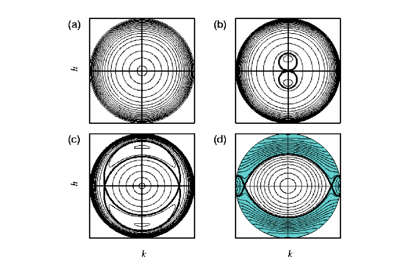
Figure 1: Contours $C={\rm{}const}$ of the first integral (12) in the plane of non-singular variables $(k,h)$. Radial distance from origin determines mean eccentricity $\bar{e}$ according to eqs. (13)–(14). Polar angle (measured from the horizontal $k$-axis) is the argument of pericentre $\bar{\omega}$. A separatrix (thick curve) is drawn on the border between regions of different topology in panels (b)–(d); there is no separatrix in (a). Contour lines with polar angle acquiring values in the full range of $0\leq\bar{\omega}\leq 2\pi$ correspond to a zone of circulation, while some values of $\bar{\omega}$ are not allowed in zones of libration. In this example, Kuzmin’s disc with $A=75$ (in units normalized by half of gravitational radius of the central mass) has been assumed. Graphs are shown for four values of Kozai’s integral respresenting topologically different situations: (a) $c=0.9$ ($0\leq\bar{e}\leq 0.436$); (b) $c=0.81$ ($0\leq\bar{e}\leq 0.586$) — notice a figure of 8-shaped separatrix between the libration and circulation regions; (c) $c=0.7$ ($0\leq\bar{e}\leq 0.714$) — notice the appearance of the second (inner) circulation region around the origin; (d) $c=0$ ($0\leq\bar{e}\leq 1$). In all these cases, trajectories have semimajor axis ${\bar{a}}=200$. Shaded area indicates highly eccentric orbits which must be trapped by the central object at some stage. More details are given in the text.

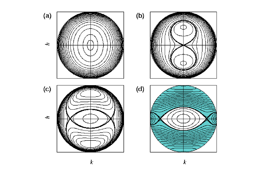
Figure 2: The same as in Figure 1 but for orbits with a smaller semimajor axis, ${\bar{a}}=75$. Values of Kozai’s integral are: (a) $c=0.9$; (b) $c=0.84$; (c) $c=0.7$; (d) $c=0$.

$$\delta\mn@boldsymbol{v}=\Sigma(R,\mn@boldsymbol{v})\,\mn@boldsymbol{v}_{\rm rel}$$ (3)

with $\Sigma(R,\mn@boldsymbol{v})=-\pi\zeta\mathchar 11131\relax(R_{\star}^{2}/m_{\star})(v_{\rm{rel}}/v_{\perp})$, and $\zeta\approx 1+(v_{\star}/v)^{4}\ln\Lambda$. Here, $\mn@boldsymbol{v}_{\rm rel}$ denotes the relative velocity of the star with respect to the disc matter, $R$ is the radial coordinate in the disc, $R_{\star}$ stellar radius, $m_{\star}$ its mass and $v_{\star}$ the escape velocity from surface of the star; $v_{\perp}$ is the normal component of the star’s velocity to the disc plane, and $\ln\Lambda$ is the long-range interaction factor. Obviously, the latter term is to be considered for transonic flows only, i.e. when the Mach number ${\cal M}\approx(R/H)>1$ (this condition is well-satisfied in standard thin accretion discs of Shakura & Sunyaev 1973; cf. also Zurek et al. 1994 who estimate the amount of the disc material swept out of the disc by a star’s passages). Finally, $H$ is the geometrical thickness of the accretion disc at distance $R$. Ostriker (1983) gives a rough estimate of $\Lambda\approx(H/R_{\star})(v/v_{\star})^{2}$. Again, for standard thin discs one obtains $\Lambda\gg 1$. We note again that the main concern is not to underestimate the role of the hydrodynamic drag. We shall thus rather conservatively assume that the factor $\zeta$ is equal to $10^{3}$.

It is worth mentioning that Artymowicz (1994) proved formula (3) approximates also the interaction of the star with density and bending waves excited on the disc surface by the star itself (see also Hall, Clarke & Pringle 1996). This additional effect can be accommodated by an appropriate modification of the drag factor $\zeta$. Taking into account an upper estimate on $\zeta$, we effectively include this effect in our considerations too.

To conclude this paragraph, we recall that the factor $\Sigma$ in eq. (3) is proportional to the surface density and therefore depends linearly on the total mass of the disc (given the density profile). When expressed in units of the central mass: $\Sigma\propto\mu$ with a numerical factor depending uniquely on the characteristics of the moving object (neutron star, white dwarf, stripped star, etc.) and of the disc material. Though simplified, this model reflects the intuitive guess that more mass in the disc makes the effects of the hydrodynamic drag more profound.

3 Evolution of stellar orbits

Hereinafter, we examine stellar orbits. First, we discuss how the gravity of the disc influences individual trajectories (Sec. 3.1). This will help us to illustrate the main differences with respect to previous works (especially, Rauch 1995). Next, we consider the combined effect of the disc gravity and the drag due to collision with the disc material (Sec. 3.2). In both cases, we will integrate orbits numerically and then we will describe orbital evolution in terms of osculating Keplerian elements. The elements relevant for our work are: semimajor axis $a$, eccentricity $e$, inclination $I$ with respect to the disc plane ($I>90^{\rm{o}}$ corresponds to retrograde orbits while $I<90^{\rm{o}}$ corresponds to prograde orbits), and argument of pericentre $\omega$ as measured from the ascending node. The longitude of the node does not appear in the following discussion because of the axial symmetry of gravitational field. The (assumed) small value of the disc-mass parameter $\mu$ and the value of $\zeta$ guarantee that the time-scale of the orbital evolution is much longer than period of a single revolution. Therefore, we will average relevant quantities over individual revolutions around the centre whenever it is appropriate. One can verify that $\mu$ controls the ratio of medium vs. short time-scale while $\zeta$ affects the ratio of long vs. medium time-scale. We accept physically substantiated values for $\mu$ ($\mathrel{\hbox to0.0pt{\lower 3.0pt\hbox{$\mathchar 536\relax$}\hss}\raise 2.0pt\hbox{$\mathchar 316\relax$}}10^{-3}$) and $\zeta$ (1–$10^{3}$) which guarantee that the three time-scales are well-separated from each other.

3.1 Effects of the disc gravity

The motion of cosmic objects in gravitational fields of discs or rings of matter has been considered in the context of solar system studies (e.g., Ward 1981; Heisler & Tremaine 1986; Lemaitre & Dubru 1991; McKinnon & Leith 1995), recently discovered planetary systems (Holman, Touma & Tremaine 1997), and in galactic dynamics (Huang & Carlberg 1997).

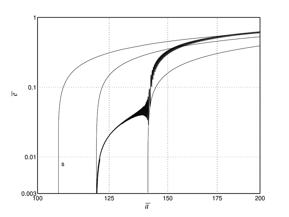
Figure 3: Mean eccentricity $\bar{e}$ vs. semimajor axis $\bar{a}$. The curly curve corresponds to the trajectory from the first example in sec. 3.2. Both axes are logarithmic. Kuzmin’s disc model with scaling parameter $A=75$ and mass parameter $\mu=10^{-3}$ has been used. Initial semimajor axis $\bar{a}=200$, eccentricity $\bar{e}=0.6$, inclination $\bar{I}=34.4\degr\!\!$, and argument of pericentre $\bar{\omega}=90\aas@@fstack{\circ}$ For sake of comparison, three hypothetical orbits, evolution of which disregards gravitational influence of the disc, are also plotted (monotonic curves); one of these curves (labeled by “s”) corresponds to the same initial conditions as the complete solution.

As mentioned above, we are interested in the long-term variations of orbits around a massive centre and a much less massive disc. The averaging technique is a very useful approach for understanding the qualitative behaviour of the system (Arnold 1989). It can be formalized in terms of a series of successive canonical transformations in which rapidly changing variables (e.g. mean anomaly along the osculating ellipse) are eliminated (Brouwer & Clemence 1961). Since the reader may not be closely familiar with this technique we briefly remind several basic concepts.

Suppose we consider motion of a particle in the Keplerian field, determined by an integrable Hamiltonian $H_{0}$ and a weak perturbation. Perturbation is described by a potential $\epsilon V$. The parameter $\epsilon$ indicates a smallness of the perturbation (in our case, the disc/hole mass ratio $\mu$ plays the role of $\epsilon$). Hamiltonian of the central field in terms of the Keplerian elements reads $H_{0}=-GM_{\rm{}c}/(2a)$, depending uniquely on the semimajor axis, while the perturbing potential $V$ depends, in general, on all Keplerian parameters. For this reason, a general solution cannot be found but the the problem is simplified when some symmetry appears. For instance, the axial symmetry induces independence on the longitude of node. Since the averaging technique is based on canonical transformation theory one should rather use a set of canonical elements of the two-body problem. Delaunay parameters are the most common choice (see, e.g., Brouwer & Clemence 1961).

In order to grasp the long-term evolution of the system one needs to get rid of the “fast” (i.e. rapidly changing) variables. In our problem there is the only one fast variable: the mean anomaly. The idea of the averaging method is then formalized by seeking a set of new Delaunay variables using a canonical transformation under the constrain of independence of the transformed Hamiltonian on this fast variable. It is possible, indeed, by formal development in the small parameter $\epsilon$. The original perturbing potential $V$ reads, after the transformation,

$$\epsilon V\;\rightarrow\;\epsilon{\bar{V}}=\epsilon{\bar{V}}_{1}+\epsilon^{2}{\bar{V}}_{2}+\epsilon^{3}{\bar{V}}_{3}+\cdots\;.$$ (4)

Various iterative and computer-algebra adapted methods for recursive generation of the potentials ${\bar{V}}_{1}$, ${\bar{V}}_{2}$, etc. were developed (e.g. Hori 1966; Deprit 1969). We note that the first term in this series, notably ${\bar{V}}_{1}$, is just the average of the original potential $V$ over the mean anomaly. Obviously, a rigorous proof of convergence of the series (4), and thus a success of the whole procedure, remains a very difficult task. Despite of this fact the averaging technique is often very useful. Typically, results based even on highly truncated part of this series are valid on a limited time interval though they fail to predict the system’s evolution on an infinite time-scale. In many applications such a weakened demand is sufficient (see, for instance, Milani & Knežević 1991 for the application to a long-term evolution of asteroidal orbits).

Regarding the independence of the new Hamiltonian on the fast variable (i.e. mean anomaly) we immediately conclude that the mean perturbing potential ${\bar{V}}$ is the first integral of motion:

$$\epsilon{\bar{V}}=\epsilon{\bar{V}}_{1}+\epsilon^{2}{\bar{V}}_{2}+\epsilon^{3}{\bar{V}}_{3}+\ldots=\epsilon C(\epsilon)\;.$$ (5)

Factorizing out the small parameter $\epsilon$ one can see that the first order perturbing function, ${\bar{V}}_{1}$, is nearly constant — provided that the higher order contribution is neglected. Notice that the right-hand side constant $C$ is a function of the small parameter $\epsilon$. However, in the most truncated level of averaging, accounting for the first order term of the right hand side of (4) only, we have

$${\bar{V}}_{1}\approx C(0)+{\cal O}(\epsilon)\;,$$ (6)

and the averaged perturbation potential ${\bar{V}}_{1}$ is (approximately) constant. In the following we shall drop out the argument (which is zero) and write $C$ for simplicity. In the case of an axially symmetric system the integral (6) is sufficient for global integrability. Now the problem is reduced to a single degree of freedom and the whole phase space can be plotted in a simple two-dimensional graph. Qualitative features of the solution can be illustrated by isocurves of the $C$-integral (6).

In the remaining part of this section we shall apply the previous brief review of the averaging to our problem. We shall restrict ourselves to the first-order procedure in which the perturbation potential $V_{\rm{}d}$ is substituted by its average $\bar{V}_{\rm{}d}$ over the mean anomaly:

$$\bar{V}_{\rm{}d}=\frac{1}{2\pi\eta}\int_{0}^{2\pi}{\rm{d}}v\left(\frac{r}{\bar{a}}\right)^{2}V_{\rm{d}}({R},z),$$ (7)

where $r$, ${R}$, and $z$ are functions of true anomaly $v$, $\eta=\sqrt{1-\bar{e}^{2}}$ ($\bar{e}$ denotes mean eccentricity of the orbit). One can write, in terms of mean inclination $\bar{I}$ and mean argument of pericentre $\bar{\omega}$,

$$r = \frac{\bar{a}\eta^{2}}{1+\bar{e}\cos v},$$ (8)

$$z = r\sin\bar{I}\sin\left(\bar{\omega}+v\right),$$ (9)

$${R} = r\sqrt{1-\sin^{2}\bar{I}\sin^{2}\left(\bar{\omega}+v\right)}.$$ (10)

At this level of approximation, the mean semimajor axis $\bar{a}$ stays constant and differs from the osculating semimajor axis $a$ by short-period terms only. Owing to axial symmetry of $\bar{V}_{\rm{}d}$ there exists an additional first integral of motion which relates ${\bar{I}}$ to the corresponding value of ${\bar{e}}$ in the course of their evolution,

$$\sqrt{1-\bar{e}^{2}}\cos\bar{I}=c\equiv{\rm{}const}\,.$$ (11)

Eq. (11) is often called Kozai’s integral (Kozai 1962). Here again, the overbar distinguishes the mean elements from the corresponding osculating elements. The problem is reduced to the evolution of ${\bar{e}}$ and ${\bar{\omega}}$ which are constrained by

$${\bar{V}}_{\rm{}d}\left({\bar{e}},{\bar{\omega}};c,{\bar{a}}\right)=C\,.$$ (12)

We will introduce a pair of non-singular canonical variables $(k,h)$:

$$k = \sqrt{2(1-\sqrt{1-{\bar{e}}^{2}})}\cos{\bar{\omega}},$$ (13)

$$h = \sqrt{2(1-\sqrt{1-{\bar{e}}^{2}})}\sin{\bar{\omega}};$$ (14)

$(k,h)$ are often called Poincaré variables, since they have been introduced to orbital dynamics by Poincaré (1892). Levels of $C={{\rm{}const}}$ in the $(k,h)$-plane offer a convenient representation of the long-term evolution of mean orbital elements. At small values of eccentricity ${\bar{e}}$, the radial distance from the origin in the $(k,h)$-plane is equal to the mean eccentricity itself, while the polar angle has the meaning of the argument of pericentre ${\bar{\omega}}$. The final task is to evaluate the averaged potential, ${\bar{V}}_{\rm{}d}\left({\bar{e}},{\bar{\omega}};c,{\bar{a}}\right)$. Since we are interested in averaging over orbits which intersect the disc, no simple analytical techniques based on expansion in orbital elements (common in celestial mechanics) can be applied to a general distribution of surface density $\mathchar 11131\relax(R)$ (see the Appendix). Even in the case of simple Kuzmin’s discs (2) the averaging cannot be performed in analytical functions and must be obtained numerically.

Figure 1 illustrates contours $C={{\rm{}const}}$ of the first integral (12) in the case of a Kuzmin disc with scaling parameter $A=75$. The size of orbit is characterized by a value of mean semimajor axis ${\bar{a}}=200$. Geometrized units of length have been used; in the following, we will use half of the gravitational radius of the central object as a natural unit of length (this choice is motivated by interpreting the central object as a black hole; otherwise, our discussion is Newtonian).

Kozai’s integral $c$ spans the whole interval $(-1,1)$, but we can restrict ourselves to positive values because $c$ occurs in ${\bar{V}}_{\rm{}d}$ only squared. Large values of $c$ (Fig. 1a, $c=0.9$) correspond to quasi-circular orbits with low inclination to the disc plane and small oscillations in mean eccentricity. The argument of pericentre circulates in the whole interval $(0,2\pi)$. When $c$ is decreased (Fig. 1b, $c=0.7$), larger inclinations occur and two regions of libration with associated stable points at $\bar{\omega}=\pm\pi/2$ develop and bifurcate into a figure of 8-shaped region. Orbits outside this libration region still circulate with $0\leq\bar{\omega}\leq 2\pi$ ($0$ is to be identified with $2\pi$). Notice that circulating trajectories which are close to the separatrix of the two regions exhibit large oscillations in the mean eccentricity. At still smaller values of $c$ (Fig. 1c, $c=0.2$), the circulation region bifurcates in its inner part near origin. Stable points in the libration regions are expelled farther to higher eccentricities. Setting $c=0$ (Fig. 1d) the inclination is constrained to $\bar{I}=\pi/2$ (polar orbits). There is a maximum eccentricity above which the orbits are trapped by the central object (this situation corresponds to a pericentre distance equal to $2$ in our example). We observe that a large portion of the plot (indicated by shading) corresponds to orbits which emerge from or fall into the centre, while only a very minor part — namely the inner circulation region with a stable point $\bar{e}=0$ — contains orbits which survive the long-term evolution. In the following, this property turns out to be essential for the fate of orbits counter-rotating with respect to the disc. We will argue that most initially retrograde orbits cannot last long enough to be tilted over the polar orbit and inclined into the disc plane because, in course of this process, their eccentricity is being pumped up to such a high value that they get captured by the central object.

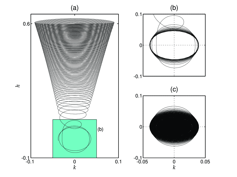
Figure 4: Long-term evolution of the orbit from Figure 3 projected onto the $(k,h)$-plane. Initial librations around the fixed point at $\bar{\omega}=90\degr$ are shown in panel (a). As the Kozai’s parameter $c$ increases, the libration zone shrinks and the orbit approaches the separatrix. Eventually, the orbit crosses the separatrix and starts circulating around the origin; see continuation of orbital evolution in panel (b). Still further continuation in (c) shows that the orbit terminates in the inner zone of circulation, with zero eccentricity.

Figure 2 shows the same graphs as in Figure 1 but for different ratio of the scaling parameters of density distribution ($A=75$, as before) and the orbit ($\bar{a}=75$, changed). All features in the $(k,h)$-plane described before stay unchanged except the fact that libration regions and the inner zone of circulation cover a larger portion of the graphs. At small values of Kozai’s integral we again observe that eccentricity is forced to large oscillations which eventually lead to capture (shaded area).

We have verified that qualitatively similar results hold for different, astrophysically relevant disc density–potential pairs. In particular, using formulae from the Appendix we have numerically computed potential of discs with $R^{-1}$, $R^{-2}$ and $R^{-3}$ surface density laws and then averaged over corresponding quasi-elliptic orbits.

3.2 Influence of star-disc collisions

We now consider inclusion in our model of the influence of the hydrodynamic drag affecting the orbit when the star crosses the accretion disc. We will use the approximations described in Sec. 2.2, and, for definiteness, we will assume that the central cluster of stars is formed by white dwarfs or stripped cores of ordinary stars and use relevant parameters for estimating numerical factor in the relation $\Sigma\propto\mu$ (eq. [3] above). Before embarking on a description of our results, we recall that Rauch (1995) has considered long-term evolution of stellar orbits in which he took into account the impulsive drag acting twice per revolution only (no gravity of the disc; see also previous studies by Syer et al. 1991, and Vokrouhlický & Karas 1993, 1998).

All stellar orbits interacting with the disc, independently of their initial conditions, exhibit long-term decay of the semimajor axis, and monotonous decrease of eccentricity and inclination (grinding to the disc plane). For initially low-inclination orbits, the characteristic time-scale of circularization is comparable to the grinding time after which the orbital plane becomes inclined into the disc. Orbits with large initial inclination, in particular all initially retrograde orbits, are circularized before they incline to the disc. Rauch (1995) argues that, for orbits with an initially moderate eccentricity, a particular combination of the mean elements, $\bar{a}(1-{\bar{e}}^{2})\cos^{4}({\bar{I}}/2)$, is quasi-conserved in the course of evolution (see also Vokrouhlický & Karas 1998). This property is insensitive to a particular model of the star-disc interaction, surface density profile, and the total mass of the disc. For further use we recall the way that the hydrodynamical drag affects the mean semimajor axis ${\bar{a}}$ and the Kozai parameter $c$ (two integrals of the long-term evolution when star-disc interactions are neglected): due to the drag effect, $\bar{a}$ undergoes permanent decay while $c$ typically increases from its initial value to the final value of $c_{\rm f}=1$, corresponding to a circular orbit in the disc plane. Initially retrograde orbits behave in a somewhat different way: their circularization time-scale is significantly shorter than the grinding time. For these orbits, the value of Kozai’s parameter first slightly decreases before exhibiting monotonous increase to $c_{\rm{}f}$.

The main result of the present paper is that most of the above-mentioned properties cease to be true in our generalized model which, besides star-disc collisions, includes also the gravitational influence of the disc matter. The key point is the fact that the characteristic time-scale $\bar{a}/\dot{\bar{a}}\approx\bar{c}/\dot{\bar{c}}$ of the hydrodynamical-drag effects is much longer than the characteristic time-scale for circulation and libration of pericentre. Circulation and libration along $C={\rm{}const}$ lines are due to the disc gravity, and the corresponding period is also the time-scale for gravity-driven oscillations in eccentricity and inclination. As a consequence, the principal features of orbital variations explained in the previous section remain unchanged apart from a very slow adiabatic evolution of quasi-integrals $(\bar{a},c)$. However slow this evolution is, stellar orbits are strongly and abruptly affected at some stages: when they cross the separatrix (due to some perturbation) or when the libration region bifurcates. In the following paragraphs we will illustrate these facts by showing typical orbits. Kuzmin’s disc with $A=75$ has been assumed in examples described below. The mass of the disc has been set to $\mu=10^{-3}$ for definiteness (units of the central mass). It should be mentioned that the results depend only very weakly on the particular value of $\mu$, provided it is sufficiently small. The reason emerges from the fact that the disc-mass parameter can be factorized out of all expressions containing the averaged potential ${\bar{V}}_{\rm d}$ (which determines all important dynamical features). On the other hand, and in contrast to the results of Rauch (1995), one expects dependence on the surface density profile $\mathchar 11131\relax(R)$.

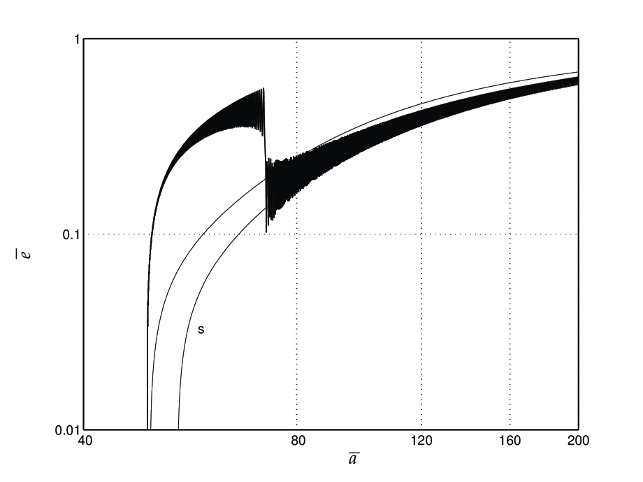
Figure 5: Eccentricity $\bar{e}$ vs. semimajor axis $\bar{a}$ (the second example in sec. 3.2). The same parameters of the disc as in Figure 3, different initial parameters of the orbit: $\bar{a}=200$, $\bar{e}=0.67$, $\bar{I}=67\degr\!\!$, and $\bar{\omega}=0$. Again, the gravitation of the disc induces oscillations and an abrupt increase of eccentricity (curly curve) which cannot be seen when the disc gravity is neglected (two monotonic curves).

In the first example of this section, we consider an orbit with the initial parameters: $\bar{a}=200$ (in units of one half of the gravitational radius), $\bar{e}=0.6$, $\bar{I}=34.4\degr$ ($c\approx 0.66$), and $\bar{\omega}=90\aas@@fstack{\circ}$ Figure 3 shows mean eccentricity $\bar{e}$ as a function of the semimajor axis $\bar{a}$ during the course of orbital evolution. For sake of comparison we have also plotted three curves of orbital evolution if the gravitational influence of the disc is ignored. These curves can be compared directly with corresponding results of Vokrouhlický & Karas (1993) and Rauch (1995). The curve labeled by “s” corresponds to the same initial conditions as the orbit of the complete model with gravitational effects taken into account (notice the difference in predicted radius of the terminal orbit); the other two curves correspond to different initial eccentricities. As expected from the previous discussion, the most evident features are (i) large oscillations in eccentricity, and (ii) permanent decay of the semimajor axis. The radius of the resulting circularized orbit in the disc plane, $a_{\rm{}f}=120.2$, differs slightly from the estimation based on Rauch’s (1995) formula, $a_{\rm{}f}^{\rm{R}}\approx{}a_{\rm{}i}(1-e_{\rm{}i}^{2})\cos^{4}{}I_{\rm{}i}/2=106.5$. A closer look at orbital evolution explains a remarkable bump in eccentricity near $\bar{a}\approx 141$. In the initial state, the pericentre of the orbit librates in one of the two lobes of the 8-shaped zone, around $\bar{\omega}=90\degr\!\!$, as shown in Figure 4a. As the Kozai parameter $c$ slowly increases due to the hydrodynamic drag the libration zone shrinks and the orbit approaches the separatrix. At a particular instant, the orbit is expelled from the libration zone, crosses the separatrix and enters the zone of circulation (see Figure 4b). This transition is accompanied by large oscillations of the mean eccentricity and temporal slowing down of the eccentricity decay.

Our second example of the orbital evolution (Figure 5) appears even more peculiar (from the viewpoint of previous results neglecting gravity of the disc). Initial orbital parameters are as follows: $\bar{a}=200$ , $\bar{e}=0.638$, $\bar{I}=67\degr$ ($c\approx 0.3$), and $\bar{\omega}=0$. The first part of the orbital evolution ends at $a\approx 71.5$ by a significant increase of mean eccentricity. The oscillations of eccentricity eventually settle down and the evolution terminates as a circular orbit in the disc plane, $a_{\rm{}f}\approx{}49.2$. The latter radius is to be compared with Rauch’s approximative result: $a_{\rm{}f}^{\rm{R}}\approx{}54.3$. Obviously, this estimate fails to predict the final radius correctly but the difference is still within uncertainty of Rauch’s quasi-integral (Vokrouhlický & Karas 1998). Again, a closer look at the evolution of pericentre in the $(k,h)$-plane sheds light on properties of this model. Initially the orbit is confined to the inner zone of circulation around the origin (Figure 6). An adiabatic increase of Kozai’s parameter results in collapse of this zone and the orbit is expelled towards the separatrix. At the instant of crossing the separatrix, the orbit may either enter the libration zone surviving for larger values of $c$, or it terminates in the large circulation zone. It can be argued, that orbits close to the separatrix spend most of their time near the hyperbolic points which leads preferentially to the capture in the circulation zone. This indeed happened in our example, as indicated by a thick line in Figure 6. The form of the 8-shaped libration zone results in significant increase of eccentricity. Figure 7 shows a projection of the orbit onto the plane of mean eccentricity $\bar{e}$ and inclination $\bar{I}$. One can notice that individual oscillations are confined to the underlying grid of constant Kozai’s integral (11). Slow (adiabatic) diffusion across the lines $c={\rm{}const}$ reflects a long-term feature of the orbital evolution. Transition from the inner to the outer circulation zones is accompanied by a large increase of eccentricity, but only a moderate decrease of inclination.

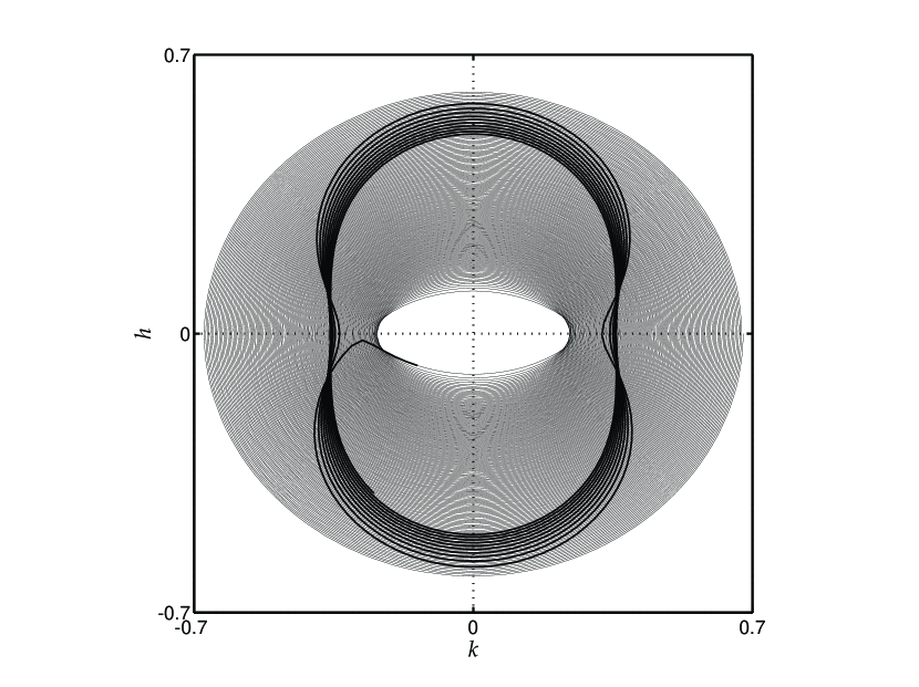
Figure 6: Orbital evolution from Figure 5 projected onto the $(k,h)$-plane. Initial circulation in the inner zone of circulation (thin curve) is followed by transition to the external zone of circulation (thick curve) at a critical value $c\approx 0.78$ of the Kozai parameter. At this moment eccentricity is increased back to a high value. Notice also a reversal of the sense of circulation.

So far we have demonstrated the intricate role of the disc gravity in evolution of stellar orbits with initially prograde inclination ($I_{\rm{}i}<90\degr$). Even though details of the orbital evolution are different when compared to models neglecting disc gravity, overall features remain approximately unchanged. Most importantly, radii of circularized orbits in the disc plane are comparable. However, as mentioned before, one has to pay particular attention to orbits with initially large, retrograde inclination where the results become qualitatively and quantitatively different. Two subsequent examples deal with this class of orbits.

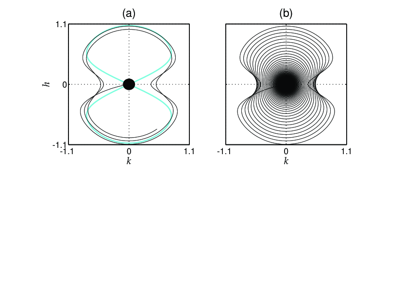
Figure 9: Long-term evolution of the orbit from Figure 8 projected onto the $(k,h)$-plane. Evolution in the inner zone of circulation is shown in panel (a), until the trajectory escapes to the outer zone of circulation. Form of the 8-shaped separatrix is indicated at the moment of transition to high eccentricity. Subsequent evolution continues in panel (b) with a steady decrease of eccentricity. The trajectory eventually approaches the origin of the $(k,h)$ plane.

Figure 8 corresponds to an initially retrograde orbit with parameters: $\bar{a}=200$, $\bar{e}=0.1$, $\bar{I}=120\degr$ ($c\approx-0.5$), and $\bar{\omega}=90\aas@@fstack{\circ}$ Similar to the previous example, this orbit is originally locked in the inner zone of circulation. This is necessary (but insufficient as we shall see later) if the orbit is to be tilted over the polar orbit to a prograde one and survive further evolution. Otherwise, it gets captured rather soon by the central mass. Just before the separatrix of the inner circulation zone shrinks to origin, the orbit is released to the outer zone of circulation. The existence of the libration lobes then leads to significant increase of the mean eccentricity, up to $0.9$. The $(k,h)$-plane representation of the orbit evolution is given in Figure 9. The circular equatorial orbit with radius $a_{\rm{}f}\approx{}7.8$ is a final state of this evolution. Its radius is to be compared with $a_{\rm{}f}^{\rm{R}}\approx{}12.4$ (no gravity of the disc). The difference between terminal radii predicted by the two models amounts to $30\,$%. Starting with various initial conditions we found that terminal radius and corresponding time are comparable, typically within factor of 2.

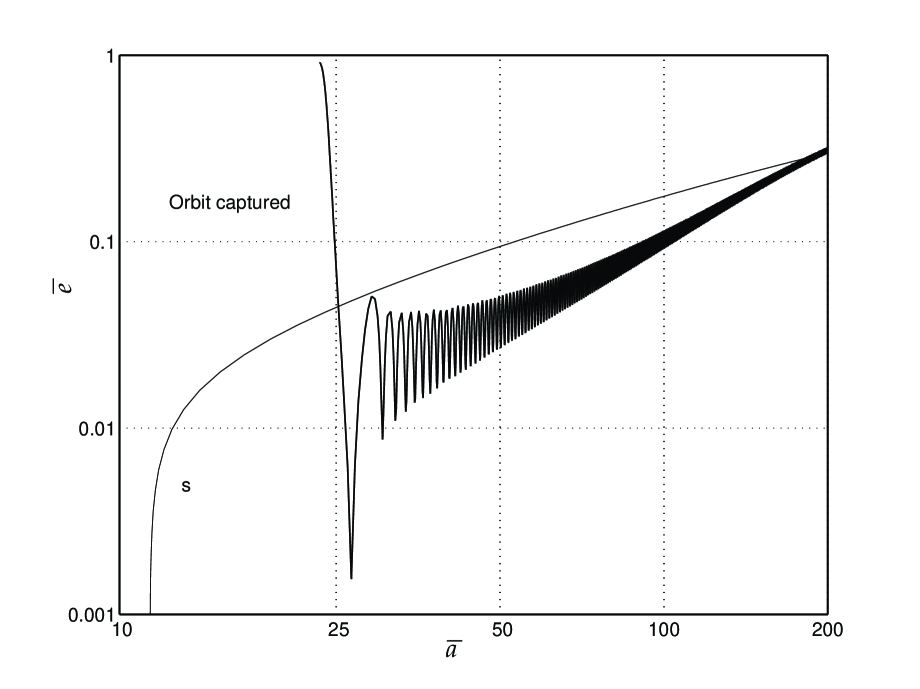
Figure 10: Eccentricity $\bar{e}$ vs. semimajor axis $\bar{a}$ (the fourth example in sec. 3.2; initially retrograde orbit). The same disc and orbit parameters as in Figure 8 except for the initial mean eccentricity $\bar{e}=0.3$. The orbit which follows from our complete model has been captured by the central mass due to a large increase of eccentricity at the moment of transition from the inner to the outer zone of circulation, while the simplified model orbit grinded down safely to the equatorial plane.

A truly fundamental difference between the complete model, with the disc gravity taken into account, and the simplified model, disregarding effects of the disc gravity, is observed when the initial eccentricity of the previous orbit is slightly increased to $0.3$. The corresponding orbital evolution is shown in Figure 10. The orbit is again initially locked in the inner zone of circulation. But now, at the transition to the outer circulation zone, eccentricity increases over a critical level and the orbit is captured by the central object (pericentre is less than $2$). On the contrary, a hypothetical orbit with no gravity of the disc grinds to the disc plane at final radius $a_{\rm{}f}\approx{}11.4$. Concerning retrograde orbits, we can conclude that even those ones that have started within the inner zone of circulation are not safe from capture (obviously, orbits with larger initial eccentricity than $0.3$ in our example are also captured). We have also verified that retrograde orbits which are initially locked in the libration lobes or in the outer circulation zone do not survive tilting over the polar orbit, being soon captured by the centre due to large oscillations in eccentricity. All these orbits are grinded safely to the equatorial plane in the framework of the simplified model of Rauch (1995), when the disc gravity is neglected. We would like to stress again that this difference is not based on the particular value of the disc mass we have chosen in our examples ($\mu=10^{-3}$); rather it is present for an arbitrary nonzero mass of the disc (naturally, evolution takes place on a longer time-scale for smaller values of $\mu$). The same results hold also for less massive discs.

A theoretical substantiation for the reported $\mu$-independence of our results is based on existence of the quasi-integral (6) mentioned above. Notice that the small parameter $\epsilon$ (i.e. $\mu$ in our case) can be factorized from this formula. Only when the higher-order terms of the exact integral (5) are taken into account the results (phase portraits, in particular) depend on $\mu$. As soon as $\mu$ is sufficiently small, which means smaller than about $10^{-3}$ in practice, the averaging technique offers a simple explanation for the $\mu$-insensitivity of the results.

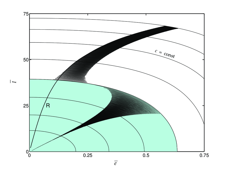
Figure 7: Mean inclination $\bar{I}$ vs. mean eccentricity $\bar{e}$ of the orbit from Figure 5. Background grid of constant values of the Kozai parameter, $c={\rm{}const}$, is also plotted. Orbital evolution consists of fast oscillations along the lines of $c={\rm{}const}$ and slow diffusion towards the maximum value of $c_{\rm{}f}=1$ ($\bar{e}=\bar{I}=0$). Kozai’s quasi-integral is not isolating because the transition between the inner and the outer (shaded) circulation zones crosses one of the $c={\rm{}const}$ curves. Rauch’s solution is also shown by the monotonic curve (labeled by “R”).

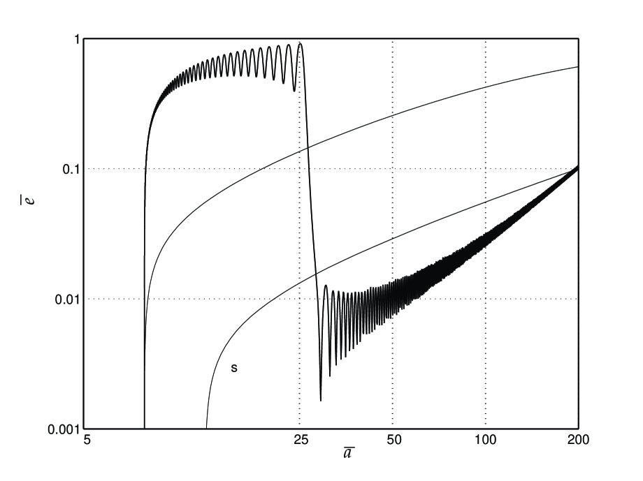
Figure 8: Mean eccentricity $\bar{e}$ vs. semimajor axis $\bar{a}$ (the third example in the text; an initially retrograde orbit). The same parameters of the disc as in Figure 3; starting parameters of the orbit are as follows: $\bar{a}=200$, $\bar{e}=0.1$, $\bar{I}=120\degr\!\!$, and $\bar{\omega}=90\aas@@fstack{\circ}$ Complete model orbit is represented by a curly curve with oscillations in eccentricity, while the two orbits of a simplified model (no gravity of the disc) exhibit monotonic decrease of eccentricity during the whole evolution.

We have verified our principal conclusions for discs with different surface density profiles. In particular, we considered stellar orbits around discs with density profiles proportional to $R^{-1}$, $R^{-2}$, and $R^{-3}$. Obviously, the values of parameters when transitions between zones in the $(k,h)$-plane occurred are quantitatively different in individual cases, but what holds unchanged are the qualitative results. Most importantly, a significant fraction of the initially retrograde orbits is captured by the central mass.

3.3 Notes on statistical properties of the cluster

In this section, we briefly comment on possible influence of our results on statistical properties of a cluster of stars near a galactic nucleus.

The important finding, in this respect, concerns the significant portion of orbits which increase eccentricity and than become captured by the centre, many of them being initially retrograde. These orbits are missing in the final configuration of the system. The form of this final configuration appears to be sensitive to the detailed nature of the situation under consideration. Rauch (1995) specified the initial distribution of stars as a power-law in binding energy. Then the system evolved under interactions with a disc for infinite time, stellar orbits were inclined into the disc plane or captured by the centre, and the index of the power-law has been evolved accordingly. No new stars have been inserted into the system. Since retrograde orbits end up with smaller radii in the disc plane than initially prograde ones [due to the term $\cos^{4}(I/2$) in Rauch’s estimate], we expect in our model deficiency of orbits very close to the central object when compared to the results of Rauch. As a consequence a softer power law of the final distribution is to be expected in comparison to the Rauch’s work.

Alternatively, one can look for equilibirum in which the number density of stars remains constant at all radii. Stars which get captured by the central mass must be substituted by new ones which come from infinite radius. Now it is important to take into account the fact that time interval for grinding the orbit into the disc depends on initial inclination (it is longer for initially retrograde orbits than for prograde). Discussion in this section is to be verified by detailed numerical simulations (work in progress).

4 Conclusions

It has been recognized by previous works that statistical properties of central galactic clusters are influenced by an accretion disc surrounding the nucleus because of twice-per-revolution interaction which affects stellar motion. The main results of this paper can be summarized as follows:

(i)

we demonstrated that any consistent model of the star-disc interaction has to take the influence of the disc gravity into account, in addition to the effects of direct collisions with gaseous material;

(ii)

as a result of the disc gravity, individual stellar orbits exhibit evolution which is different if compared to the situation when collisions are considered but gravity neglected. Most importantly, we found that a significant fraction of initially retrograde (i.e. counter-rotating with respect to the disc material) orbits are captured by the central object. This is due to large oscillations in eccentricity which affect polar orbits.

We wish to note that our two findings mentioned above are to some extent different in their nature. The former one — (i) — is essentially a statement of consistency claiming that any reasonable model which involves the effects of direct star-disc physical interaction has to take disc gravity also into account. We argued that this claim is valid for all astrophysically reasonable objects expected in central clusters of galaxies: neutron stars, white dwarfs and stripped stars. The logic behind this result is due to the fact that both effects are controlled by the total mass of the disc. The latter finding — (ii) — then states how the model supplemented by effects of the disc gravity differs from previous simpler models. Gravity of the disc induces dynamical structures, libration and circulation zones of the argument of pericentre. Adiabatic change of quasi-integral quantities and related transitions of trajectories between the two zones are the essence of our results.

It is worth recalling that the above-mentioned results did show sensitivity on a particular model of the disc, especially on the radial gradient of the surface density. Indeed, while Rauch (1995), considering only star-disc collisions, reported his results to be insensitive to a particular profile of the surface density or even to the model of the star-disc interaction, we observed that the fraction of retrograde orbits captured by the central mass in the course of their evolution depends on details of both star-disc collisions and effects of the disc gravity. On the other hand, our results show only a weak sensitivity on the total mass of the accretion disc. This feature can be easily understood by realizing that the disc mass parameter $\mu$ factorizes out (in the first order of approximation) from the averaged potential ${\bar{V}}_{\rm d}$. As a consequence, the value of $\mu=10^{-3}$ taken in our examples in Sec. 3 is not essential, and similar results hold also for less massive discs.

Note: we have prepared a Java animation which illustrates long-term evolution of stellar orbits in the two zones of the $(k,h)$-plane (libration and oscillation in eccentricity); cf. “http://astro.troja.mff.cuni.cz/karas/papers/discapplet.html”.

We are grateful to Richard Stark and the unknown referee for very helpful suggestions concerning the presentation of our article. We acknowledge support from grants GA CR 205/97/1165 and GA CR 202/96/0206 in the Czech Republic. V. K. is grateful for kind hospitality of the International Centre for Theoretical Physics and International School for Advanced Studies in Trieste where this work was completed.

Appendix A Gravitational field of a thin disc

In this section we describe a general method for evaluating the gravitational potential, and its gradient, of an axisymmetric disc. We introduce cylindrical coordinates $({R},z,\phi)$ with origin in the centre of the disc and the plane $z=0$ coinciding with the disc plane. The gravitational potential of the disc (outer radius $b_{\rm{}d}$) evaluated at arbitrary position $({R},z)$ is given by (see, e.g., Binney & Tremaine 1987)

$$V_{\rm{}d}\left({R},z\right)=-\,4G\int_{0}^{b_{\rm{}d}}\frac{\mathchar 11131\relax({R^{\prime}}){R^{\prime}}}{B({R^{\prime}})}K\left[k\left({R^{\prime}}\right)\right]\,{\mbox{d}}{{R^{\prime}}}\,,$$ (15)

where

$$k^{2}\left({R^{\prime}}\right)=\frac{4{R}{R^{\prime}}}{B^{2}({R^{\prime}})}\,,$$ (16)

and

$$B^{2}\left({R^{\prime}}\right)=z^{2}+\left({R}+{R^{\prime}}\right)^{2}\,.$$ (17)

Here, $K(k)$ is the elliptic integral of the first kind. (The dependence of functions $B({R^{\prime}})$ and $k({R^{\prime}})$ on coordinates ${R}$ and $z$ is not indicated explicitly.)

No apparent reduction of integral (15) is possible until the radial distribution of the density $\mathchar 11131\relax({R^{\prime}})$ is specified. An important example which we will need below is a uniform disc, $\mathchar 11131\relax({R^{\prime}})\equiv\mathchar 11131\relax_{0}$. The potential (15) expressed in terms of elliptic integrals $K$, $E$ and $\Pi$ reads, for ${R}<b_{\rm{}d}$, (Lass & Blitzer 1983)

$$V_{\rm{}d}({R},z)_{\mid\mathchar 11131\relax=\mathchar 11131\relax_{0}}\,\equiv\,V_{\rm{}u}\left({R},z;\mathchar 11131\relax_{0}\right)$$ (18)

$$= 2G\mathchar 11131\relax_{0}\biggl{\{}\pi|z|-B\left(b_{\rm{}d}\right)E\left[k\left(b_{\rm{}d}\right)\right]-\frac{b_{\rm{}d}^{2}-{R}^{2}}{B\left(b_{\rm{}d}\right)}K\left[k\left(b_{\rm{}d}\right)\right]$$

$$-\frac{b_{\rm{}d}-{R}}{b_{\rm{}d}+{R}}\frac{z^{2}}{B\left(b_{\rm{}d}\right)}\,\Pi\left[\alpha^{2};k\left(b_{\rm{}d}\right)\right]\biggr{\}}$$

with

$$\alpha^{2}=\frac{4b_{\rm{}d}{R}}{(b_{\rm{}d}+{R})^{2}}\,.$$ (19)

Formula (18) holds also in the region ${R}>b_{\rm{}d}$ provided the first term in brackets of the right-hand side is suppressed. The expression for the potential inside the disc $(z=0,$ ${R}<b_{\rm{}d})$ can be simplified by applying the Gauss transformation of elliptic functions (Byrd & Friedman 1971). One finds that

$$V_{\rm{}u}({R},0;\mathchar 11131\relax_{0})=-4Gb_{\rm{}d}\mathchar 11131\relax_{0}E\left({R}/b_{\rm{}d}\right)\,,$$ (20)

a more compact formula than the one given by Lass & Blitzer (1983).

The components of gravitational force are given by the gradient of the potential (15). Direct algebraic manipulation results in

$$\frac{\partial V_{\rm{}d}}{\partial{R}} = -\frac{2G}{{R}}\int_{0}^{b_{\rm{}d}}\frac{\mathchar 11131\relax({R^{\prime}}){R^{\prime}}}{B({R^{\prime}})}\biggl{\{}E\left[k\left({R^{\prime}}\right)\right]\frac{{R^{\prime}}^{2}-{R}^{2}+z^{2}}{A^{2}\left({R^{\prime}}\right)}$$ (21)

$$-K\left[k\left({R^{\prime}}\right)\right]\biggl{\}}\,{\mbox{d}}{{R^{\prime}}}\,,$$

$$\frac{\partial V_{\rm{}d}}{\partial z} = -4Gz\int_{0}^{b_{\rm{}d}}\frac{\mathchar 11131\relax({R^{\prime}})\,{R^{\prime}}\,E\left[k\left({R^{\prime}}\right)\right]}{B({R^{\prime}})\,A^{2}\left({R^{\prime}}\right)}\,{\mbox{d}}{{R^{\prime}}}\,,$$ (22)

where we denoted

$$A^{2}\left({R^{\prime}}\right)=z^{2}+\left({R}-{R^{\prime}}\right)^{2}\,.$$ (23)

For a uniform disc one obtains

$$\frac{\partial V_{\rm{}u}}{\partial{R}} = -\frac{2G\mathchar 11131\relax_{0}}{{R}B\left(b_{\rm{}d}\right)}\Bigl{\{}B^{2}\left(b_{\rm{}d}\right)E\left[k\left(b_{\rm{}d}\right)\right]$$ (24)

$$-\left(z^{2}+b_{\rm{}d}^{2}+{R}^{2}\right)K\left[k\left(b_{\rm{}d}\right)\right]\Bigr{\}}\,,$$

$$\frac{\partial V_{\rm{}u}}{\partial z} = 2G\mathchar 11131\relax_{0}\biggr{\{}\pm\pi-\frac{z}{B\left(b_{\rm{}d}\right)}\Bigl{(}K\left[k\left(b_{\rm{}d}\right)\right]$$ (25)

$$+\frac{b_{\rm{}d}-{R}}{b_{\rm{}d}+{R}}\,\Pi\left[\alpha^{2}\left(b_{\rm{}d}\right);k\left(b_{\rm{}d}\right)\right]\Bigr{)}\biggr{\}}\,.$$

The integrands in eqs. (15) and (21)–(22) diverge in the disc plane, $z\rightarrow 0,$ although the result of integration must be finite because the potential is continuous across the disc. Taking into account relation

$$K(k)\propto\ln\left(1-k^{2}\right)$$ (26)

for $k\approx 1$, one concludes the divergence in the potential is proportional $\ln z$. To get rid of numerical errors one conveniently splits the integrals into two parts by setting $\mathchar 11131\relax({R^{\prime}})\equiv[\mathchar 11131\relax({R^{\prime}})-\mathchar 11131\relax({R})]+\mathchar 11131\relax({R})$. Then the potential is

$$V_{\rm{}d}\left({R},z\right) = -4G\int_{0}^{b_{\rm{}d}}\frac{\left[\mathchar 11131\relax({R^{\prime}})-\mathchar 11131\relax({R})\right]{R^{\prime}}}{B({R^{\prime}})}\,K\left[k\left({R^{\prime}}\right)\right]\,{\mbox{d}}{{R^{\prime}}}$$ (27)

$$+V_{\rm{}u}\left[{R},z;\mathchar 11131\relax({R})\right]\,,$$

where the second term corresponds to the potential of the disc with constant density $\mathchar 11131\relax({R})$ given by eq. (18). Now the integrand in (27) is well behaved. A sharp decrease of the integrand near ${R^{\prime}}\approx{R},$ $z\approx 0$ can be treated by appropriate numerical methods. The same approach can be applied successfully to evaluate the components of force in eqs. (21)–(22).

Previous formulae are easily generalized to the case when the inner edge of the disc is at radius $a_{\rm{}d}\neq 0$. The lower integration limit in (15) and (21)–(22) is changed to $a_{\rm{}d}$, and in the case of formulae (18) and (24)–(25) for the uniform density disc one employs a superposition of the field of a fictitious uniform disc with radius $a_{\rm{}d}$ and formal density $-\mathchar 11131\relax_{0}$.

References

- [Ambartsumian 1938] Ambartsumian V. A., 1938, Ann. Leningrad State Univ., 22, 19
- [Arnold 1989] Arnold V. I., 1989, Mathematical Methods of Classical Mechanics, (Springer-Verlag, Berlin)
- [Artymowicz 1994] Artymowicz P., 1994, ApJ, 423, 581
- [Artymowicz, Lin & Wampler 1993] Artymowicz P., Lin D. C. N., Wampler E. J., 1993, ApJ, 409, 592
- [Bahcall & Wolf 1976] Bahcall J. N., Wolf R. A., 1976, ApJ, 209, 214; 1977, ibid, 216, 883
- [Binney & Tremaine 1987] Binney J., Tremaine S., 1987, Galactic Dynamics, (Princeton University Press, Princeton)
- [Bondi & Hoyle 1944] Bondi H., Hoyle F., 1944, MNRAS, 104, 274
- [Brouwer & Clemence 1961] Brouwer D., Clemence G., 1961, Methods of Celestial Mechanics, (Academic Press, New York)
- [Byrd & Friedman 1971] Byrd P. F., Friedman M. D. 1971, Handbook of Elliptic Integrals for Engineers and Scientists, (Springer-Verlag, Berlin)
- [Chandrasekhar 1944] Chandrasekhar S., 1942, Principles of Stellar Dynamics, (Univ. of Chicago Press, Chicago)
- [Courvoisier & Mayor 1990] Courvoisier T. J.-L., Mayor M. (eds.), 1990, Active Galactic Nuclei, (Springer-Verlag, Berlin)
- [Deprit 1969] Deprit A., 1969, Celest. Mech., 1, 12
- [Evans & de Zeeuw 1992] Evans N. W., de Zeeuw P. T., 1992, MNRAS, 257, 152
- [Frank & Rees 1976] Frank J., Rees M. J., 1976, MNRAS, 176, 633
- [Goldreich & Tremaine 1980] Goldreich P., Tremaine S., 1980, ApJ, 241, 425
- [Hagio 1987] Hagio F., 1987, PASJ, 39, 887
- [Hall, Clarke & Prongle 1996] Hall S. M., Clarke C. J., Pringle J. E., 1996, MNRAS, 278, 303
- [Hameury et al. 1994] Hameury J.-M., King A. R., Lasota J.-P., Auvergne M., 1994, AA, 292, 404
- [Heisler 1986] Heisler J., Tremaine S., 1986, Icarus, 65, 13
- [Holman et al. 1997] Holman M., Touma J., Tremaine S., 1997, Nat, 386, 254
- [Hori 1966] Hori G., 1966, PASJ, 18, 287
- [Hoyle & Lyttleton 1939] Hoyle F., Lyttleton R. A., 1939, Proc. Camb. Phil. Soc. 35, 592.
- [Huang & Carlberg 1997] Huang S., Carlberg R. G., 1997, ApJ, 480, 503
- [Kozai 1962] Kozai Y., 1962, AJ, 67, 591
- [Lass & Blitzer 1983] Lass H., Blitzer L., 1983, Cel. Mech., 30, 225
- [Lee & Ostriker 1993] Lee H. M., Ostriker J. P., 1993, ApJ, 409, 617
- [Lemaitre & Dubru 1991] Lemaitre A., Dubru P., 1991, Cel. Mech., 52, 57
- [Lin & Ida 1997] Lin D. N. C., Ida S., 1997, ApJ, 477, 781
- [Livio et al. 1991] Livio M., Soker N., Matsuda T., Anzer U., 1991, MNRAS, 253, 633
- [Marconi et al. 1997] Marconi A., Axon D. J., Macchetto F. D., Capetti A., Sparks W. B., Crane P., 1997, MNRAS, in press
- [McKinnon & Leith 1995] McKinnon W. B., Leith A. C., 1995, Icarus, 118, 392
- [Milan 199] Milani A., Knežević Z., 1991, Celest. Mech., 49, 347
- [Nolthenius & Katz 1982] Nolthenius R. A., Katz J. L., 1982, ApJ, 263, 377
- [Novikov, Pethick & Polnarev 1992] Novikov I. D., Pethick C. J., Polnarev A. G., 1992, MNRAS, 255, 276
- [Novikov & Thorne 1973] Novikov I. D. & Thorne K. S., 1973, in Black Holes, eds. DeWitt C., DeWitt B. S., (Gordon and Breach, New York), p. 343
- [Ostriker 1983] Ostriker J. P., 1983, ApJ, 273, 99
- [Peebles 1972] Peebles P. J. E., 1972, ApJ, 178, 371
- [Perry & Williams 1993] Perry J., Williams R., 1993, MNRAS 260, 437
- [Petrich et al. 1989] Petrich L. I., Shapiro S. L., Stark R. F., Teukolsky S. A., 1989, ApJ, 336, 313
- [Pineault & Landry 1994] Pineault S., Landry S., 1994, MNRAS, 267, 557
- [Podsiadlowski & Rees 1994] Podsiadlowski P., Rees M. J., 1994, in: The Evolution of X-ray binaries, eds. S. S. Holt & C. S. Day, (AIP Press, New York)
- [Poincare 1892] Poincaré H., 1892, Les Méthodes Nouvelles de la Mécanique Céleste, Vol. I (Gauthier-Villars, Paris)
- [Quinlan, Hernquist & Sigurdsson 1995] Quinlan G. D., Hernquist L., Sigurdsson S., 1995, ApJ, 440, 554
- [Rauch 1995] Rauch K. P., 1995, MNRAS, 275, 628
- [Shakura & Sunyaev 1973] Shakura N. I., Sunyaev R. A., 1973, AA, 24, 337
- [Shapiro & Teukolsky 1985] Shapiro S. L., Teukolsky S. A., 1985, ApJ, 292, L41; 1986, ibid, 307, 575
- [Sigurdsson & Rees 1997] Sigurdsson S., Rees M. J., 1997, MNRAS, 284, 318
- [Sigurdsson et al. 1995] Sigurdsson S., Hernquist L., Quinlan G. D., 1995, ApJ, 446, 75
- [Spitzer 1940] Spitzer L., 1940, MNRAS, 100, 397
- [Statler et al. 1987] Statler T. S., Ostriker J. P., Cohn H., 1987, ApJ, 316, 626
- [Syer et al. 1992] Syer D., Clarke C. J., Rees M. J., 1991, MNRAS, 250, 505
- [Takeda et al. 1985] Takeda H., Matsuda T., Sawada K., Hayashi C., 1985, Progress Theor. Physics, 74, 272
- [Urry & Padovani 1995] Urry C. M., Padovani P., 1995, PASP, 107, 803
- [Vokrouhlický & Karas 1993] Vokrouhlický D., Karas V., 1993, MNRAS, 265, 365
- [Vokrouhlický & Karas 1998] Vokrouhlický D., Karas V., 1998, MNRAS, 293, L1
- [Ward 1981] Ward W. R., 1981, Icarus, 47, 234
- [Young 1980] Young P. J., 1980, ApJ, 242, 1232
- [Zamir 1993] Zamir R., 1993, ApJ, 403, 278
- [Zurek et al. 1994] Zurek W. H., Siemiginowska A., Colgate S. A., 1994, ApJ, 434, 46; 1996, ibid, 470, 652