[

The Impact of Inhomogeneous Reionization on
Cosmic Microwave Background Anisotropy

Abstract

It is likely that the reionization of the Universe did not occur homogeneously. Using a model that associates ionized patches with overdense regions, we find that the resulting cosmic microwave background (CMB) anisotropy power spectrum peaks at angular scales corresponding to the extent of the ionized regions, and has a width that reflects the correlations between them. There is considerable uncertainty in the amplitude. Neglecting inhomogeneous reionization in the determination of cosmological parameters from high resolution CMB maps may cause significant systematic error.

] Introduction. Observations of cosmic microwave background (CMB) anisotropy are providing strong constraints on theories of cosmological structure formation. Planned CMB observations can potentially provide constraints on the parameters of these theories at the percent level[1, 2]. One of the reasons the CMB is such a wonderful probe of cosmological parameters is that predictions for a given theory can be made with great precision[3]. This is because linear perturbation theory is an excellent approximation over the relevant length scales at $z\simeq 1100$ when the CMB was last tightly coupled to matter.

However, new anisotropies can be generated at late times by the non-linear process of reionization as the CMB photons are brought back into contact with matter via Thomson scattering. We know this reionization took place before redshift $z\simeq 5$ because spectra of distant quasars do not show a continuum of absorption by neutral hydrogen. It is unlikely that reionization occurred at $z\mathrel{\mathchoice{\lower 3.6pt\vbox{\halign{$\mathsurround=0pt\displaystyle\hfil#\hfil$\cr>\crcr\sim\crcr}}}{\lower 3.6pt\vbox{\halign{$\mathsurround=0pt\textstyle\hfil#\hfil$\cr>\crcr\sim\crcr}}}{\lower 3.6pt\vbox{\halign{$\mathsurround=0pt\scriptstyle\hfil#\hfil$\cr>\crcr\sim\crcr}}}{\lower 3.6pt\vbox{\halign{$\mathsurround=0pt\scriptscriptstyle\hfil#\hfil$\cr>\crcr\sim\crcr}}}}60$ for in that case the level of anisotropies on degree scales would be significantly lower than on ten degree scales, when actually just the opposite is true [4].

Reionization affects the CMB in several ways. First, the fluctuation power on small angular scales is damped by a factor $e^{-2\tau}$ where $\tau$ is the optical depth back to last scattering. Second, as Sunyaev and Kaiser [5] pointed out, secondary anisotropies are generated on large scales due to the Doppler effect when photons scatter off moving free electrons. They also noted that the effect is strongly suppressed on small scales because photons get nearly opposite Doppler shifts on different sides of a density peak, a consequence of potential flows generated by gravitational instability. Both of these effects—the damping and the Sunyaev-Kaiser (SK) effect—are linear and therefore included in standard Boltzmann codes[3].

Here we focus on the effects of inhomogeneities in the ionization field [6, 7, 8]. We show that inhomogeneous reionization (IHR) restores the SK effect at small scales due to modulation of the velocity field with the spatial variation of the ionization fraction, an effect analogous to the modulation by the density field in the homogeneous case at second order in perturbation theory[9]. Since the typical patch size is much smaller than the scale of variation of the velocity field, the Doppler effect contributions come only from regions where the flow is coherent. The resulting anisotropy pattern depends sensitively on the model of reionization. Thus, the signature of IHR in the CMB provides an indirect window on a poorly probed but interesting era in which the first stars and galaxies formed. On the other hand, if these anisotropies are large enough, they can create systematic errors in the determination of cosmological parameters. So, after calculating the anisotropies, we compute the magnitude of these systematic errors, i.e. how much a given cosmological parameter might be misestimated if IHR is ignored.

Anisotropy Spectrum: Formal Solution. The perturbation to the photon temperature distribution function, $\Delta\equiv\delta T/T$, is governed by the Boltzmann equation, which at the late times of interest is

$$\partial\Delta({\bf x},\eta,\hat{\gamma})/\partial\eta=n_{e}\sigma_{T}a\hat{\gamma}\cdot\bf v(\bf x,\eta)$$ (1)

where $a=(1+z)^{-1}$ is the scale factor of the universe normalized to unity today, $\eta\equiv\int dt/a$ is the conformal time, $n_{e}$ is the free electron density, $\sigma_{T}$ is the Thomson cross-section, $\hat{\gamma}$ is the direction of the photon momentum, and $\bf v$ is the electron velocity. Henceforth we work in units where the conformal time today is unity, $\eta_{0}=1$; and assume a flat, matter dominated universe, $a=\eta^{2}$. The solution to Eq. 1 for the photon perturbations here and now (at ${\bf x}={\bf x}_{0}$ and $\eta=1$; $\Delta_{0}(\hat{\gamma})\equiv\Delta({\bf x}_{0},\eta_{0},\hat{\gamma})$ ) is

$$\Delta_{0}(\hat{\gamma})=4.06\times 10^{-5}\ \Omega_{b}h\int_{\eta_{i}}^{1}\frac{d\eta}{\eta^{3}}\ x_{e}({\bf x},\eta)\ \hat{\gamma}\cdot{\hbox{\BF v}}({\bf x}),$$ (2)

where, ${\bf v}({\bf x},\eta)\equiv-2\eta\ {\hbox{\BF v}}({\bf x})$ (Mpc/h), $n_{e}=\bar{n}_{e}\ x_{e}({\bf x},\eta)a^{-3}$, and $\bar{n}_{e}\sigma_{\rm T}\eta_{0}=0.122\Omega_{b}h$, with $\bar{n}_{e}$ the present mean electron density, $\Omega_{b}$ the baryon density in units of the critical density and $h$ the Hubble constant in units of 100 km s^-1 Mpc^-1. Both $x_{e}$ and v are evaluated at ${\bf x}={\bf x}_{0}-\hat{\gamma}(1-\eta)$, the position at time $\eta$ of a photon with direction vector $\hat{\gamma}$ incident on us today. Note that the integral includes all contributions starting from $\eta_{i}$, a time far after standard recombination at $\eta\simeq 0.03$, but before reionization occurs.

We focus on predicting the two-point correlation function, $C(\theta)\equiv\langle\Delta_{0}(\hat{\gamma})\Delta_{0}(\hat{\gamma}^{\prime})\rangle$ where $\cos\theta\equiv\hat{\gamma}\cdot\hat{\gamma}^{\prime}$ and the angular brackets indicate an average over all locations ${\bf x}_{0}$. Using Eq. 2 we obtain the correlation function due to reionization:

$$C(\theta)=10^{-12}\Big{(}\frac{\Omega_{b}h}{0.025}\Big{)}^{2}\int_{\eta_{i}}^{1}\frac{d\eta}{\eta^{3}}\int_{\eta_{i}}^{1}\frac{d\eta^{\prime}}{\eta^{\prime 3}}{\cal C}(\eta,\eta^{\prime},\theta).$$ (3)

It is therefore determined by an integral over adjacent lines of sight of the four-point correlation function

$${\cal C}(\eta,\eta^{\prime},\theta)\equiv\hat{\gamma}_{i}\hat{\gamma}^{\prime}_{j}\ \langle x_{e}x_{e}^{\prime}v_{i}v^{\prime}_{j}\rangle,$$ (4)

where, for example, $x_{e}^{\prime}\equiv x_{e}(\bf x^{\prime},\eta^{\prime})$. Different models of reionization will lead to different four-point functions. We now explore several possibilities.

Homogeneous Reionization. The simplest possibility is that reionization takes places homogeneously. While not particularly plausible, it is a useful limiting case for demonstrating the SK cancellation. In homogeneous reionization (HR), $x_{e}\equiv\bar{x}_{e}(\eta)$, where $\bar{x}_{e}$ is fraction of the Universe that is ionized. Thus we have:

$${\cal C}^{\rm HR}(\eta,\eta^{\prime},\theta)=\bar{x}_{e}\bar{x}_{e}^{\prime}\ C_{v}(\eta,\eta^{\prime},\theta)$$ (5)

and we take $\bar{x}_{e}$ to be zero at times earlier than $z_{i}+\delta z_{i}$, unity at times later than $z_{i}$ and to increase linearly with redshift during the transition. The velocity correlation function can be written as

$$C_{v}(\eta,\eta^{\prime},\theta)=\Psi_{\perp}\cos\theta+\left(\Psi_{\parallel}-\Psi_{\perp}\right){({\bf r}\cdot\hat{\gamma})\ ({\bf r}\cdot\hat{\gamma}^{\prime})\over r^{2}},$$ (6)

where $\bf r\equiv\bf x-\bf x^{\prime}$. The correlation functions of the velocity components parallel and perpendicular to $\bf r$ are

$$\Psi_{\parallel}(r) = \int\frac{P(k)}{k^{2}}\ \Big{[}j_{0}(kr)-2\frac{j_{1}(kr)}{kr}\Big{]}\ d^{3}k,$$ (7)

$$\Psi_{\perp}(r) = \int\frac{P(k)}{k^{2}}\ \frac{j_{1}(kr)}{kr}\ d^{3}k,$$ (8)

where $P(k)$ is the matter power spectrum, throughout assumed to be that of the standard cold dark matter theory [10]. Fig. 1 shows $C_{v}(\eta,\eta^{\prime},0)$ as a function of $\eta$ for fixed $\eta^{\prime}=0.188$. $C_{v}$ is strongly peaked at equal times, where the two lines of sight share the same velocity. On the other hand, at large $|\eta-\eta^{\prime}|$, $C_{v}$ becomes negative due to infall from opposite sides into an overdense region. The integration, in Eq. 3, of this oscillatory function with the slowly-varying $\bar{x}_{e}\bar{x}_{e}^{\prime}$ leads to a cancellation of Doppler effects, as described by Kaiser[5] in Fourier space.

Uncorrelated Inhomogeneous Reionization. The SK cancellation can be avoided if the velocity two-point function $C_{v}$ is modulated by the spatial dependence of $x_{e}$. To demonstrate this effect, we adopt a toy model of the reionization process: independent sources turn on randomly and instantaneously ionize a sphere with comoving radius $R$ and volume $V_{R}$, which then remain ionized. The resulting four-point function can be written as:

$${\cal C}^{\rm uc}(\eta,\eta^{\prime},\theta)=C_{v}(\eta,\eta^{\prime},\theta)\ \left[C_{x_{e}}^{\rm uc}(\eta,\eta^{\prime},\theta)+\bar{x}_{e}\bar{x}_{e}^{\prime}\right].$$ (9)

Since $\bar{\chi}$ (where $\chi\equiv 1-x_{e}$) is equal to the probability that no ionizing source is within volume $V_{R}$, the probability that no source is within $R$ of either ${\bf x}$ or ${\bf x^{\prime}}$ is (at equal times) $\langle\chi\chi^{\prime}\rangle=\bar{\chi}^{(2V_{R}-V(r))/V_{R}}=\bar{\chi}\bar{\chi}\bar{\chi}^{-V(r)/V_{R}}$ where for $r<2R$, $V(r)=V_{R}\ [1-(3/4)\ (r/R)+(1/16)\ (r/R)^{3}]$ is the overlap volume of the spheres centered on ${\bf x}$ and ${\bf x^{\prime}}$. Therefore, with the proper generalization to unequal times, we have:

$$C_{x_{e}}^{\rm uc} \equiv \langle x_{e}x_{e}^{\prime}\rangle-\bar{x}_{e}\bar{x}_{e}^{\prime}=\langle\chi\chi^{\prime}\rangle-\bar{\chi}\bar{\chi}^{\prime}$$ (10)

$$= \bar{\chi}\bar{\chi}^{\prime}\left[\bar{\chi}({\rm min}(\eta,\eta^{\prime}))^{-V(r)/V_{R}}-1\right]$$ (11)

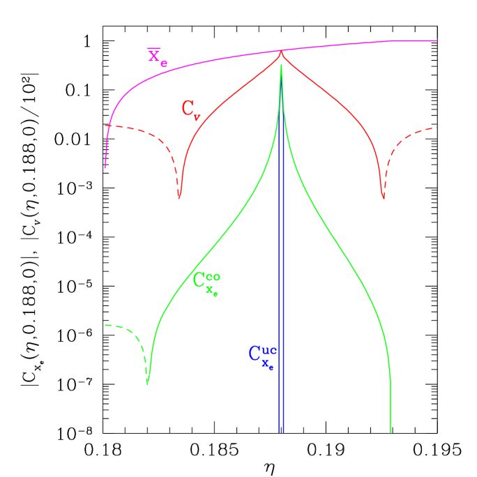
FIG. 1.: The mean ionization fraction $\bar{x}_{e}$ for HR ($z_{i}=26$, $\delta z_{i}=4$), the velocity two-point function $C_{v}(\eta,0.188,0)$ for the SCDM (standard cold dark matter) model with $\sigma_{8}=1.2$ where $\sigma_{8}$ is the rms of mass fluctuations in spheres of radius $8h^{-1}$ Mpc today, and the ionization fraction two-point function for uncorrelated $C_{x_{e}}^{\rm uc}$ and correlated bubbles $C_{x_{e}}^{\rm co}$. Dashed lines denote negative values.

The resulting two-point function, $C_{x_{e}}^{\rm uc}$, is sharply peaked at small $r\approx|\eta-\eta^{\prime}|$ (see Fig. 1, where $R=1$ Mpc), therefore in Eq. 9, ${\cal C}^{\rm uc}(\theta)\propto C_{v}(\eta,\eta,\theta)$. Thus, the SK cancellation of homogeneous reionization is avoided; IHR modulates the velocity field, accessing only the region where the velocity field is highly coherent. Note though that the modulation is not particularly effective since the ionization radius $R$ is typically very small, and thus only a tiny region of $\eta$ contributes. Therefore, as Gruzinov and Hu (GH)[7] have pointed out, a model of this type necessarily produces anisotropies which have amplitude proportional to $R$.

Figure 2 shows the anisotropy spectrum arising from the two-point function of Eq. 11, assuming $z_{i}=26$ and $\delta z_{i}=4$. The GH results for the same parameter choices would each have peaks 30% lower in $l$ and two times larger in amplitude due to a slower fall off of $C_{x_{e}}^{\rm uc}$ with $r$ and one less factor of $(1-\bar{x}_{e})$ in their version of Eq. 11. Despite these differences, they correctly identified the qualitative features of this type of IHR: (i) amplitude proportional to $R$; (ii) white noise ($C_{l}^{\rm IHR}\propto$ constant) on large scales due to lack of correlations at $r\gg R$; and (iii) peak at $l\sim(1-\eta_{r})/R$ where reionization takes place at $\eta_{r}$. We now show that the first two of these features break down when more realistic models are considered.

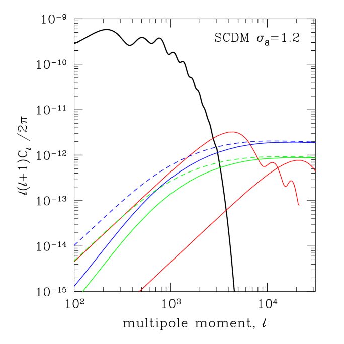
FIG. 2.: The angular power spectrum, $C_{l}$, defined by $C(\theta)\equiv\sum_{l}(2l+1)C_{l}/(4\pi)P_{l}(\cos\theta)$. The thick solid line on top is the linear spectrum. The rest are different approximations to the IHR anisotropies, all assuming $\Omega_{b}=0.1$ and $h=0.5$. The curves peaked at $l=4000$ and $l=20000$ are from the uncorrelated $R=5$ Mpc and $R=1$ Mpc models respectively. The oscillations are ringing due to the sharp cutoff of $V(r)$. The dashed curves show the model of Eq. 14 for $z_{i}=26$ (bottom) and $z_{i}=31$ (top). The remainig solid lines include velocity-ionization field cross-correlations. The correlated model curves do damp beyond $\ell\simeq 1/R>30000$.

Correlated Inhomogeneous Reionization. Because the ionizing sources in the model of Eq. 11 and that devised by GH are independent of each other, correlations in the ionization field only exist on scales comparable to, or smaller than, the ionization radius $R$. However, overdense regions, such as galaxies and clusters of galaxies, are observed to be highly correlated with each other. If overdense regions are the sources of the ionizing radiation (which they are very likely to be) then their clustering will lead to long-range correlations in the ionization field and therefore affect $C^{\rm IHR}(\theta)$.

The physical process we imagine is that the mass in any region where the linear theory density contrast smoothed on a comoving scale $R_{c}$, $\delta_{R_{c}}$, exceeds a critical threshold ($\delta_{c}=1.69$), collapses, forms stars or quasars which then ionize a region with size $R=E^{1/3}R_{c}$. The efficiency, $E$, is the ratio of the volume of the ionized regions to collapsed regions. From this scenario we expect[10, 14]

$$\bar{x}_{e} = 2E\int_{\delta_{c}}^{\infty}d\delta P_{R_{c}}(\delta)=E\ {\rm erfc}\Big{(}\frac{\delta_{c}}{\sqrt{2}\ \sigma_{R_{c}}(\eta)}\Big{)},$$ (12)

$$C_{x_{e}}^{\rm co} = \langle x_{e}x_{e}^{\prime}\rangle=\alpha\alpha^{\prime}\int_{\delta_{c}}^{\infty}d\delta\int_{\delta_{c}}^{\infty}d\delta^{\prime}\ P_{R_{c}}(\delta,\delta^{\prime})$$ (13)

$$\approx \frac{\alpha\alpha^{\prime}}{2\pi}\frac{\Xi_{R_{c}}(r)}{\sigma_{R_{c}}(\eta)\sigma_{R_{c}}(\eta^{\prime})}\exp\Big{[}-\frac{\nu^{2}(\eta)+\nu^{2}(\eta^{\prime})}{2}\Big{]},$$ (14)

where ${\rm erfc}(x)$ denotes the complementary error function, $\alpha\equiv 2E(1-\bar{x}_{e})$ (see below), $P_{R_{c}}(\delta)$ and $P_{R_{c}}(\delta,\delta^{\prime})$ are the one and two-point distributions of the smoothed field $\delta_{R_{c}}$, respectively; the smoothed correlation function is given by $\langle\delta\delta^{\prime}\rangle\equiv\Xi_{R_{c}}(r)$, $\sigma_{R_{c}}\equiv\Xi_{R_{c}}(0)$, and $\nu(\eta)\equiv\delta_{c}/\sigma_{R_{c}}(\eta)$.

Despite a number of studies of the details of reionization [11, 12, 13], we are still far from a satisfactory understanding. Therefore, we take two simple models for $E$, which can vary by many orders of magnitude (see e.g. table 2 in[12]). The requirement that objects more massive than $M_{c}(z)\simeq 10^{8}{\,M_{\odot}}[10/(1+z)]^{3/2}$ are necessary for reionization leads to a smoothing scale of $R_{c}=0.22\eta$ Mpc[13]. Our two choices for the efficiency are $E=7\times 10^{5}\ \eta^{6}$ [13], resulting in $z_{i}=26$ and $E=114$ (the “middle of the road” model in [12]), which gives $z_{i}=31$. Note that current scenarios for reionization generally lead to $E\gg 1$, i.e. the sources tend to ionize a region much larger than their typical volume (see however[8] for a different view).

Fig. 1 shows the results of Eq. 14 for the $z_{i}=26$ model. The clustering of overdense regions naturally leads to a much wider $C_{x_{e}}^{\rm co}$, which falls off only as a power-law, thus more efficiently modulating $C_{v}$. For this reason, the correlated models in Fig. 2 (dashed lines) show a much wider distribution of power, and the white noise regime is only reached at scales much larger than the patch size. Over the range of $\ell$ plotted, the power spectrum of the uncorrelated models with the same values of $R$ as in the peaks model would be orders of magnitude smaller. The dashed lines in Fig. 2 are the result of assuming $\langle x_{e}x_{e}^{\prime}vv^{\prime}\rangle=\langle x_{e}x_{e}^{\prime}\rangle\langle vv^{\prime}\rangle$ and then applying Eq. 13 for $\langle x_{e}x_{e}^{\prime}\rangle$. For the solid lines, we use an expression for $\langle x_{e}x_{e}^{\prime}vv^{\prime}\rangle$ similar to that for $\langle x_{e}x_{e}^{\prime}\rangle$ in Eq. 13 but with an integral over the joint probability distribution of $\delta,\delta^{\prime},v,v^{\prime}$[15]. This leads to a modification of the white noise behavior at large scales. Cross-correlation between HR and IHR leads to higher-order terms such as $\bar{x}_{e}\langle x_{e}^{\prime}\delta vv^{\prime}\rangle$. These are of comparable magnitude to $\langle x_{e}x_{e}^{\prime}vv^{\prime}\rangle$ and will be discussed in [15]. Note that the flatness of the power spectra in Fig. 2 above $\ell\simeq 3000$ reflects the near scale-invariance of the matter power spectrum over the relevant length scales.

Impact on Parameter Determination. The anisotropies produced during IHR may significantly affect the exquisite parameter determination anticipated from future CMB observations. Suppose a multi-dimensional fit is performed on the data to extract a set of parameters $\{p_{i}\}$. If the fit assumes $C_{l}(\{p_{i}\})$ that ignores the contribution from $C_{l}^{\rm IHR}$, then each parameter will be incorrectly estimated by an amount

$$\Delta p_{i}=F^{-1}_{ij}\sum_{l}w_{l}\ {\partial C_{l}\over\partial p_{j}}\ C_{l}^{\rm IHR}$$ (15)

where the weights $w_{l}$ are the inverse of the squares of the errors expected on $C_{l}$’s (the errors are the sum of the errors due to sample variance and those due to noise [1, 2]); $F_{ij}$ is the Fisher matrix $\sum_{l}w_{l}(\partial C_{l}/\partial p_{i})(\partial C_{l}/\partial p_{j})$. Table 1 shows the ratio of this systematic offset to the statistical uncertainty for Planck[16].

Sources of Uncertainty. Even within the context of our peaks model, Eq. 14 is not exact. Since the ionized region is larger than the region that collapsed (i.e., $E>1$) a more rigorous approach would be to calculate the probability of two points both being within a distance $R$ of one or more peaks. Instead, we have calculated the probability that two points are both within a peak and then scaled the resulting two-point function by $EE^{\prime}$. We expect this approximation to be best for $r>R$, which covers the range of relevance for the curves in Fig. 2. Because we have not taken the more rigorous approach, we must include suppression factors to correct for overcounting overlapping regions. These are the factors of $(1-\bar{x}_{e})$, motivated by their appearance in our fully tractable uncorrelated model. Removing them boosts the power spectrum by a factor of about 5.

Uncertainty in $E$ has a much milder effect on uncertainty in $C_{l}^{\rm IHR}$ than one might expect from a quick glance at Eq. 14. The reason is that increasing $E$ causes reionization to occur earlier and therefore decreases the exponential factor in Eq. 14. We find that decreasing $E$ by a factor of 10 decreases $C_{l}^{\rm IHR}$ by a factor of two.

Our peaks model, and the calculations which lead to estimates of its parameters, are highly idealized. Although more sophisticated studies will eventually alter the details of our results, we believe significant power at scales larger than the patch size is a natural consequence of cosmic structure formation via gravitational instability.

model	$n_{s}$	$r_{ts}$	$\tau$	$\Omega_{b}h^{2}$	$\Omega_{\rm vac}h^{2}$	$\Omega_{\rm m}h^{2}$	$\Omega_{\nu}h^{2}$
$z_{i}=31$	0.75	0.65	0.01	2.25	0.20	-1.02	0.94
$z_{i}=26$	0.34	0.29	0.006	1.01	0.09	-0.46	0.42

TABLE I.: Ratio of systematic offset to statistical uncertainty expected for Planck [16] from the two “peaks” models in Fig. 2. Since IHR affects very small scales, MAP [16] is much less sensitive to this offset. Variables are, from left to right, the primordial power spectrum index, the ratio of tensor to scalar contributions to $C_{2}$, the optical depth and the contribution to $h^{2}$ from (b)aryons, (curv)ature, cold dark (m)atter and massive neutrinos. The power spectrum derivatives were evaluated at the parameter values of the SCDM model in [2]. This does not include polarization information; however, since polarization is sourced by the quadrupole moment, not velocity, the polarization IHR power spectrum will be down by roughly a factor of $(10^{-5}/10^{-3})^{2}$ from the IHR temperature power spectrum.