Polarization of Microwave Background: Statistical and Physical Properties

We discuss statistical and physical properties of cosmic microwave background polarization, both in Fourier and in real space. The latter allows for a more intuitive understanding of some of the geometric signatures. We present expressions that relate electric and magnetic type of polarization to the measured Stokes parameters in real space and discuss how can be constructed locally. We discuss necessary conditions to create polarization and present maps and correlation functions for some typical models.

1 Introduction

Cosmic microwave background (CMB) anisotropies offer one of the best probes of early universe, which could potentially lead to a precise determination of a large number of cosmological parameters $\!{}^{{\bf?},{\bf?},{\bf?}}$. The main advantage of CMB versus more local probes of large-scale structure is that the fluctuations were created at an epoch when the universe was still in a linear regime. While this fact has long been emphasized for temperature anisotropies ($T$), the same holds also for polarization in CMB and as such it offers the same advantages as the temperature anisotropies in the determination of cosmological parameters. The main limitation of polarization is that it is predicted to be small: theoretical calculations show that CMB will be polarized at 5-10% level on small angular scales and much less than that on large angular scales. Future CMB missions (MAP, Planck) will have sufficient sensitivity that even such low signals will be measurable. This will allow one to exploit the wealth of information present in the polarization.

Recent work has emphasized the rich geometrical structure present in polarization $\!{}^{{\bf?},{\bf?},{\bf?}}$. In particular, linear polarization has been decomposed into electric ($E$) and magnetic ($B$) types, which transform as scalars and pseudoscalars, respectively. With polarization there are three additional power spectra that can be measured, in addition to $E$ and $B$ autocorrelation there is also $E$ and $T$ cross-correlation. Each of these can provide unique information about our universe. Most of this work has developed the formalism by using multipole expansion on a sphere or on a plane. Here we will develop some of the properties of polarization fields $E$ and $B$ directly in real space, which allows for a more intuitive understanding of their geometrical properties.

2 Statistical description of polarization

The CMB radiation field is characterized by a $2\times 2$ intensity tensor $I_{ij}$. The intensity tensor is a function of direction on the sky $n$ and two directions perpendicular to $n$ that are used to define its components (${\bf\hat{e}}_{1}$,${\bf\hat{e}}_{2}$). The Stokes parameters $Q$ and $U$ are defined as $Q=(I_{11}-I_{22})/4$ and $U=I_{12}/2$, while the temperature anisotropy is given by $T=(I_{11}+I_{22})/4$ (the factor of $4$ relates fluctuations in the intensity to those in the temperature). In color plates we represent the polarization using “vectors” with magnitude $P=\sqrt{Q^{2}+U^{2}}$ that form an angle $\alpha={1\over 2}\arctan({U\over Q})$ with ${\bf\hat{e}}_{1}$. These are not real vectors since they map into themselves after $180^{\circ}$ rotation, which is why we do not assign them a direction. In principle the fourth Stokes parameter $V$ that describes circular polarization would also be needed, but in cosmology it can be ignored because it cannot be generated through Thomson scattering. While the temperature is invariant under a right handed rotation in the plane perpendicular to direction $n$, $Q$ and $U$ transform under rotation by an angle $\psi$ as

$$Q^{\prime} = Q\cos 2\psi+U\sin 2\psi$$

$$U^{\prime} = -Q\sin 2\psi+U\cos 2\psi$$ (1)

where ${\bf\hat{e}}_{1}^{\prime}=\cos\psi\ {\bf\hat{e}}_{1}+\sin\psi\ {\bf\hat{e}}_{2}$ and ${\bf\hat{e}}_{2}^{\prime}=-\sin\psi\ {\bf\hat{e}}_{1}+\cos\psi\ {\bf\hat{e}}_{2}$. The Stokes parameters are not invariant under rotations in the plane perpendicular to $n$. For this reason it is more convenient to work with scalar and pseudoscalar polarization fields $E(\hbox{\boldmath{$n$}})$ and $B(\hbox{\boldmath{$n$}})$, respectively, which are invariant under rotations. In the small scale limit $n$ is close to $\hat{\hbox{\boldmath{$z$}}}$ and we can parametrize the direction in the sky with two-dimensional angle $\theta$ relative to a fixed coordinate system perpendicular to $\hat{\hbox{\boldmath{$z$}}}$. The two rotationally invariant fields can be written in terms of the Stokes parameters as

$$E(\hbox{\boldmath{$l$}}) = \int d^{2}{\hbox{\boldmath{$\theta$}}}\ [Q(\hbox{\boldmath{$\theta$}})\cos(2\phi_{l})+U(\hbox{\boldmath{$\theta$}})\sin(2\phi_{l})]\ e^{-i{\hbox{\boldmath{$l$}}}\cdot{\hbox{\boldmath{$\theta$}}}}$$

$$B(\hbox{\boldmath{$l$}}) = \int d^{2}{\hbox{\boldmath{$\theta$}}}\ [U(\hbox{\boldmath{$\theta$}})\cos(2\phi_{l})-Q(\hbox{\boldmath{$\theta$}})\sin(2\phi_{l})]\ e^{-i{\hbox{\boldmath{$l$}}}\cdot{\hbox{\boldmath{$\theta$}}}},$$ (2)

Here $E(\hbox{\boldmath{$l$}})$ and $B(\hbox{\boldmath{$l$}})$ are components of the two scalar fields in Fourier space. To obtain them in real space we can perform a Fourier transform

$$E(\hbox{\boldmath{$\theta$}}) = (2\pi)^{-2}\int d^{2}{\hbox{\boldmath{$l$}}}\ e^{i{\hbox{\boldmath{$l$}}}{\hbox{\boldmath{$\theta$}}}}\ E({\hbox{\boldmath{$l$}}})$$

$$B(\hbox{\boldmath{$\theta$}}) = (2\pi)^{-2}\int d^{2}{\hbox{\boldmath{$l$}}}\ e^{i{\hbox{\boldmath{$l$}}}{\hbox{\boldmath{$\theta$}}}}\ B({\hbox{\boldmath{$l$}}}).$$ (3)

These two quantities describe completely the polarization field. They can be expressed directly in terms of real space quantities $Q(\hbox{\boldmath{$\theta$}})$ and $U(\hbox{\boldmath{$\theta$}})$ as

$$E(\hbox{\boldmath{$\theta$}}) = -\int d^{2}{\hbox{\boldmath{$\theta$}}}^{\prime}\ \omega(\tilde{\theta})\ [Q({\hbox{\boldmath{$\theta$}}}^{\prime})\cos(2\tilde{\phi})-U({\hbox{\boldmath{$\theta$}}}^{\prime})\sin(2\tilde{\phi})]$$

$$= -\int d^{2}{\hbox{\boldmath{$\theta$}}}^{\prime}\ \omega(\tilde{\theta})\ Q_{r}({\hbox{\boldmath{$\theta$}}}^{\prime})$$

$$B(\hbox{\boldmath{$\theta$}}) = -\int d^{2}{\hbox{\boldmath{$\theta$}}}^{\prime}\ \omega(\tilde{\theta})\ [U({\hbox{\boldmath{$\theta$}}}^{\prime})\cos(2\tilde{\phi})+Q({\hbox{\boldmath{$\theta$}}}^{\prime})\sin(2\tilde{\phi})]$$ (4)

$$= -\int d^{2}{\hbox{\boldmath{$\theta$}}}^{\prime}\ \omega(\tilde{\theta})\ U_{r}({\hbox{\boldmath{$\theta$}}}^{\prime}).$$

The variables $(\tilde{\theta},\tilde{\phi})$ are the polar coordinates of the vector $\hbox{\boldmath{$\theta$}}-\hbox{\boldmath{$\theta$}}^{\prime}$. In equation (4) $Q_{r}$ and $U_{r}$ are the Stokes parameters in the polar coordinate system centered at $\theta$. For example, if $\theta$ is zero, $Q_{r}=\cos 2\phi^{\prime}\ Q(\hbox{\boldmath{$\theta$}}^{\prime})-\sin 2\phi^{\prime}\ U(\hbox{\boldmath{$\theta$}}^{\prime})$ and $U_{r}=\cos 2\phi^{\prime}\ U(\hbox{\boldmath{$\theta$}}^{\prime})+\sin 2\phi^{\prime}\ Q(\hbox{\boldmath{$\theta$}}^{\prime})$. The window can be shown to be $\omega(\theta)=1/\pi\theta^{2}\;(\theta\neq 0)$, $\omega(\theta)=0\;(\theta=0)$.

From equation 4 we can understand how to obtain two rotationally invariant quantities out of $Q$ and $U$ directly in real space: to obtain $E({\hbox{\boldmath{$\theta$}}})$ and $B({\hbox{\boldmath{$\theta$}}})$ we radially integrate over circles centered at $\theta$ the values of $Q_{r}$ and $U_{r}$, respectively. Each circle is weighted by $\omega({\tilde{\theta}})$. By construction these two quantities are rotationally invariant: the Stokes parameters $Q_{r}$ and $U_{r}$ do not depend on the coordinate system, as they are defined relative to the $\hbox{\boldmath{$\theta$}}-\hbox{\boldmath{$\theta$}}^{\prime}$ vector. The weight function $\omega$ is also rotationally invariant. We are giving the same weight to all the points in each circle and we are using the Stokes parameters defined in their natural coordinate system, defined parallel and perpendicular to the line joining the two points (denoted with $r$ in equation 4). The variable $B$ is clearly a pseudoscalar because it is the average of $U_{r}$ and $U_{r}$ changes sign under parity. Note that the window extends out to infinity and so the quantities $E$ and $B$ are nonlocal. This is not the only possible choice: one can construct finite extent versions of $E$ and $B$ from $Q$ and $U$ using a compensated window such that $\int\theta d\theta\ g(\theta)=0$, e.g. $\tilde{E}=\int Eg(\theta)d^{2}\theta$ and similarly for $B$. The relation between these averaged $\tilde{E}$ and $\tilde{B}$ and $Q$, $U$ is still given by equation 4 using

$$\omega(\theta)=-g(\theta)+{2\over\theta^{2}}\int_{0}^{\theta}d\theta^{\prime}\theta^{\prime}g(\theta^{\prime}).$$ (5)

We can therefore construct pure $E$ or $B$ quantities which are obtained from an integral over a finite region and test the geometrical structure of polarization without measuring the whole sky, as long as the measured field is contiguous. Note that for these real space quantities there is no need to worry about mode coupling because of incomplete sky coverage, which would for example mix some $E$ into $B$ in Fourier space.

Let us further explore properties of $E$ and $B$ type polarizations in real space. For simplicity we will continue to use small scale limit. Plate 1 shows the $E$ polarization field and the polarization vectors for a typical (standard CDM) model. There is only $E$ type polarization associated with this model, because this is the only pattern that is produced by density perturbations and we did not include a stochastic background of gravity waves. We discuss this point further below. In figure 1 and plate 1 we can see that hot spots of the $E$ map correspond to points with tangential polarization pattern (negative $Q_{r}$). Radial polarization pattern is found around the cold spots of $E$. From equation 4 we can read directly the relations between the pattern of polarization and the sign of $E$ and $B$. Note that there is a formal similarity between weak lensing and polarization: $E$ plays a role of convergence $\kappa$, while $Q$ and $U$ can be viewed as the two shear components $\gamma_{1}$ and $\gamma_{2}$. Since weak lensing is only important for scalar perturbations $B$ mode is not excited, which provides a consistency check. The sign convention for $E$ agrees with weak lensing $\!{}^{{\bf?}}$: positive mass density (positive $\kappa$) generates a tangential pattern of shear, so likewise positive $E$ gives rise to a tangential polarization pattern.

To obtain $B$ type polarization we can rotate all polarization “vectors” by $45^{\circ}$. Hot and cold spots of the $B$ field correspond to places where the polarization vectors circulate around in opposite directions (figure 1 and plate 2). It is clear from this figure that such polarization pattern is not invariant under reflections (parity transformation). This is the main distinction between $E$ and $B$ type of polarization: under parity operation $E$ transforms as a scalar and $B$ as a pseudoscalar.

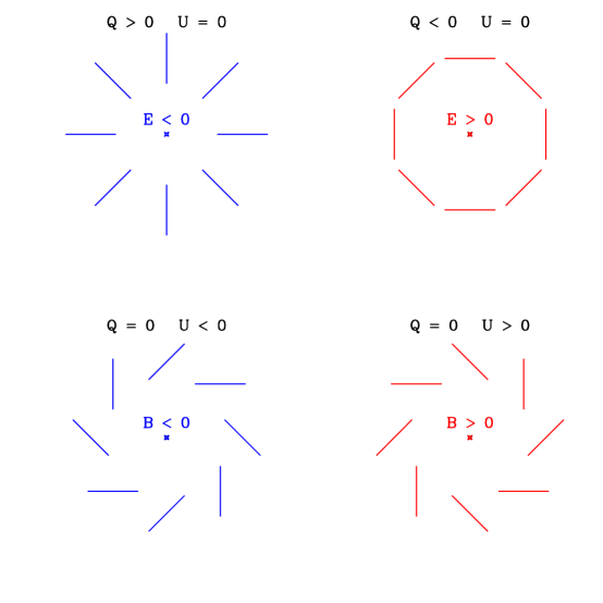
Figure 1: Polarization patterns that lead to positive and negative values of the $E$ and $B$ fields. The Stokes parameters are measured in the polar coordinate system centered at the cross. All four patterns are invariant under rotation but the two patterns that generate $B$ are not invariant under reflections.

We can now address the polarization pattern induced by different types of perturbations. In particular, we want to show why scalar perturbations cannot induce $B$ type of polarization. Without loss of generality we may consider only one Fourier mode of scalar perturbations at a time, since an arbitrary field can always be expanded in a linear superposition of Fourier modes. Let us assume we are observing in direction $n$, while the mode is oriented in direction $\hat{\bf k}$. In the plane perpendicular to $n$ we can define a local coordinate system with axis aligned parallel and perpendicular to the plane that contains both $\hat{\bf k}$ and $n$. Scalar modes have a rotation symmetry around $\hat{\bf k}$, which implies that $U=0$ in this frame (figure 2). Let us now look at the polarization pattern in the circle around direction $n$ in the plane perpendicular to it. Polarization is directed either in the direction towards $\hat{\bf k}$ or perpendicular to this direction, since only $Q$ is generated in the frame determined by that direction (for simplicity only radial case is depicted in figure 2). Polarization is invariant under the reflection across the axis determined by the $\hat{\bf k}$ and $n$ line, because polarization amplitude only depends on the angle between $\hat{\bf k}$ and $n$. Therefore any integration around this circle will produce only $E$ and not $B$. Since both $E$ and $B$ are obtained by radial averaging of contributions from individual circles and $B$ vanishes for each for each of them it follows that $B=0$ in general. By construction this is coordinate independent, hence one cannot produce $B$ polarization with scalar perturbations in general.

For tensor perturbations this argument no longer applies, as shown in figure 2. Here the amplitude of perturbation depends also on the orientation of the stretching and squeezing of space in the direction perpendicular to the direction of plane propagation (figure 2). There is no parity symmetry and both $E$ and $B$ will be generated in general. This is also true for vector modes. For these modes velocity is perpendicular to the direction of wave propagation. Its direction in the plane perpendicular to $\hat{\bf k}$ breaks the symmetry and generates $B$ modes.

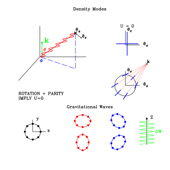
Figure 2: A single mode of density perturbations has symmetries under rotation around the $\hat{\bf k}$ axis and reflection around any plane containing it. Only $Q$ Stokes parameter can be present in this reference frame, implying no $B$ polarization is created (see the text). Gravitational waves do not have these symmetries as illustrated by the deformation suffered by a ring of test particles as wave propagating in direction $\hat{\bf k}$ passes by. There is a particular direction associated with the direction of the stretching and there is no rotational or parity symmetry. The same is true for vector modes, which induce velocities perpendicular to the wave direction.

3 Generation of Polarization

The standard picture of big bang model is that the universe was hot in the beginning and was expanding and cooling thereafter. At high temperatures electrons and protons were free in the universe, because photons were sufficiently energetic to prevent any recombination to survive. Once the energy of most of the photons dropped below 13.6eV ionization was no longer possible and at that time (at energies around 0.3eV) the universe recombined and became transparent for photons. The recombination was very rapid. Before recombination the density of free electrons was very high, so that the photon mean free path was very short. Together with electrons they formed a single fluid, with pressure provided by the photons and inertia by the baryons. This fluid supported the analog of acoustic oscillations where both the density and velocity were oscillating functions of time $\!{}^{{\bf?},{\bf?}}$. The density was proportional to $\cos(c_{s}k\tau+\delta)$, while the velocity to $\sin(c_{s}k\tau+\delta)$, where $c_{s}$ is the sound speed and the phase $\delta$ depends on initial conditions and is in general time dependent.

To generate polarization we need Thomson scattering between photons and electrons. Electric field incident on the electron causes this electron to oscillate in the direction of the field and electron radiates according to the dipole emission formula. Looking for example perpendicular to the incoming light direction only one polarization of incident light will be seen to cause electron to oscillate, the one perpendicular to the plane containing the incoming and outgoing directions. Dipole radiation emits preferentially perpendicular to the direction of oscillation, so the light we observe will be polarized. To get the total effect we need to integrate over the light intensity in all the directions. If the radiation incident on the electron is isotropic there will be no net polarization generated after the scattering, simply by symmetry. Dipole distribution also does not generate polarization. For example, consider the case where the intensity of the incident radiation is higher from the top and lower from th e bottom, with the average intensity incident from the sides. Observing from above the plane scattered light from photons incident from either the bottom or top of the plane will be polarized in the horizontal direction, while that coming from the sides will be polarized in the vertical direction. Adding up all the components we find that horizontal and vertical components are equal, implying no polarization. We therefore need a quadrupolar pattern of intensity, in which case there is an excess of horizontal polarization from both top and bottom, which does not cancel the smaller vertical polarization from the sides.

Since we need Thomson scattering it is clear that polarization cannot be generated after recombination of electrons and protons into hydrogen, when the universe becomes transparent for the photons. We still need to show however that there is sufficient quadrupole moment prior to last scattering, because only then will polarization be generated. In the electron rest frame one sees photons coming from distances of the order of a mean free path $\lambda_{p}$. The photons that are scattered off a given electron come from places where the fluid has velocity ${\bf{v}}$ and because of the tight coupling between photons and electrons the photon distribution function has a dipole term $T_{1}=\hat{{\bf n}}\cdot{\bf{v}}$. To generate quadrupole moment one requires a gradient in the velocity field across the mean free path, $T_{2}=\lambda_{p}n^{i}n^{j}\partial_{i}v_{j}$ in the rest frame of the electron. But since the mean free path was so short prior to recombination the induced quadrupole was very small, until the last moment during recombination when mean free path started to grow. This implies that the mean free path is of the order of the duration of recombination and a detailed analysis gives $\!{}^{{\bf?}}$

$$(Q+iU)(\hat{{\bf n}})\approx 0.17\Delta\tau_{*}{\bf m}^{i}{\bf m}^{j}\partial_{i}v_{j}|_{\tau_{*}},$$ (6)

where $\Delta\tau_{*}$ is the width of the last scattering surface, happening at $\tau_{*}$. The appearance of ${\bf m}=\hat{{\bf e}}_{1}+i\hat{{\bf e}}_{2}$ in equation 6 assures that $(Q+iU)$ transforms correctly under rotations of $(\hat{{\bf e}}_{1},\hat{{\bf e}}_{2})$ (equation 1).

Figure 3 shows the temperature, $E$ polarization and $T-E$ cross-correlation power spectra. The oscillations in the spectra can be understood with the tight coupling approximation described above. At the time of recombination waves of different wavevectors $k$ are at different phases in their oscillations. The phase only depends on the amplitude of the wavevector, so all the modes with the same amplitude of wavevector have the same phase. For particular values of this amplitude all the corresponding modes vanish. A given physical scale is related to the corresponding angular scale via the angular diameter distance, but the correspondence is not perfect because of 3-d to 2-d projection. If it were perfect the power spectrum of polarization would vanish at some values, but in reality it does not (figure 3). Nevertheless, the oscillations in polarization are much more pronounced than in temperature, because the latter receives contributions both from density and velocity and the two are out of phase with each other, so that even if one vanishes for some value of $k$ the other does not.

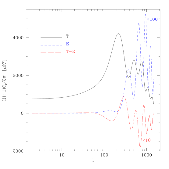
Figure 3: Power spectra for COBE normalized SCDM. The $E$ and the $T-E$ spectra have been rescaled for convenience.

On large scales polarization is strongly suppressed. Correlations over large angles can only be created by the long wavelength perturbations, but these cannot produce a large polarization because of the tight coupling between photons and electrons prior to recombination: only wavelengths that are small enough to produce anisotropies over the mean free path of the photons will give rise to a significant quadrupole in the temperature distribution, and thus to polarization. On small scales ($l\geq 1000$) both polarization and temperature anisotropies are suppressed by photon diffusion. Here the wavelength of the perturbation becomes comparable to the mean free path of the photons prior to recombination. Photons can diffuse out of density peaks smaller than a diffusion length, thereby erasing the anisotropies. Note also that there is an extra gradient in polarization relative to temperature (equation 6), which explains why polarization amplitude peaks at a smaller angular scale. The fact that the polarization field has relatively more small scale power is particularly evident when we compare the the $T$ and $E$ fields in plates 1 and 3. Finally, temperature polarization cross-correlation oscillates just like the other two spectra, but can be either positive or negative (figure 3).

Figure 4 shows the correlation functions in real space. The spectrum has been smoothed with a $\theta_{fwhm}=0.2^{o}$ gaussian, similar to the MAP beam. The correlation functions are defined in their natural coordinate system. In this frame there is no cross-correlation between $U_{r}$ and $T$. An interesting point is that both polarization auto-correlation functions are negative for some angular range, which does not happen for the temperature. To interpret the cross correlation we can consider the polarization pattern around a hot spot ($T>0$). The cross correlation starts positive, implying a radial pattern of polarization. Not all the polarization is correlated with the temperature so it is difficult to see this trend in plate 3. In plate 4 we only plot the correlated part of the polarization and here one can see more clearly that polarization “vectors” are preferentially radial around hot spots.

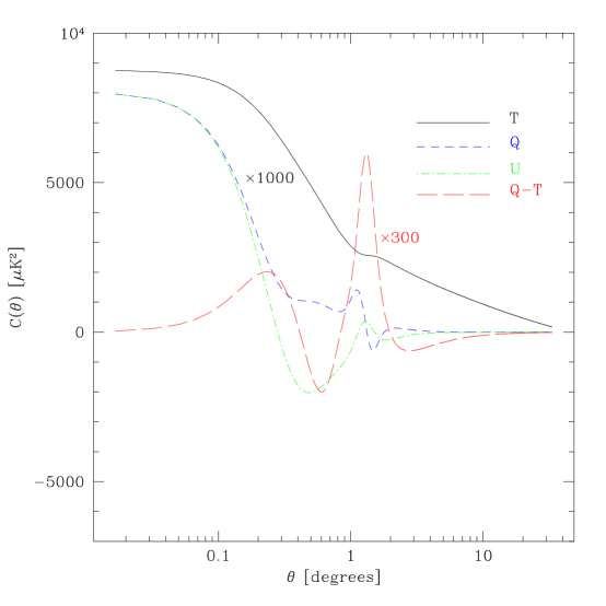
Figure 4: Correlation functions in real space for COBE normalized standard CDM model. The spectra have been smoothed with a $\theta_{fwhm}=0.2^{o}$ corresponding to the beam size of MAP.

Moving to larger angular scales the cross correlation changes sign. When it is negative the pattern becomes tangential. For large separations the polarization around a hot (cold) spot is tangential (radial). A point worth noting is that the cross correlation vanishes at $\theta=0$, in contrast to what happens for the other correlation functions. This follows simply from symmetry, since there is no preferred direction that polarization should take. Only when we consider two points separated by some distance is the symmetry broken. The vector joining the two points becomes the privileged direction and the polarization can be preferentially parallel or perpendicular to this direction.

4 Conclusions

Polarization has a rich geometrical structure, which can be simply understood using a real space construction of scalar and pseudoscalar fields. These can be constructed as integrals over Stokes $Q$ and $U$ parameters. Finite extent versions exist which allow one to search for $B$ polarization without measuring the whole sky.

Generation of polarization requires both Thomson scattering and significant quadrupole moment of photon distribution in electron rest frame. We give simple arguments why this is so and discuss predictions for some realistic models. Realistic attempts to extract polarization information have to include complications such as instrument noise and foregrounds and are given elsewhere in these proceedings $\!{}^{{\bf?}}$.

References

References

- [1] G. Jungman, M. Kamionkowski, A. Kosowsky, & D. N. Spergel, Phys. Rev. Lett. 76, 1007 (1996); Phys. Rev. D 54 1332 (1996).
- [2] J. R. Bond, G. Efstathiou & M. Tegmark, Mon. Not. R. Astron. Soc. 291, 33 (1997).
- [3] M. Zaldarriaga, D. N. Spergel & U. Seljak, Astrophys. J. 488, 1, (1997).
- [4] U. Seljak, Astrophys. J., 482 6 (1996)
- [5] M. Kamionkowski, A. Kosowsky & A. Stebbins, Phys. Rev. D 55 7368 (1997).
- [6] M. Zaldarriaga & U. Seljak, Phys. Rev. D 55, 1830 (1997).
- [7] N. Kaiser, Astrophys. J. 388, 272 (1992).
- [8] U. Seljak, Astrophys. J. 435, L87 (1994).
- [9] W. Hu & N. Sugiyama, Phys. Rev D 51, 2599 (1995).
- [10] M. Zaldarriaga & D. Harari, Phys. Rev D 52, 3276 (1995).
- [11] S. Prunet, S. K. Sethi & F. R. Bouchet, these proceedings; S. K. Sethi, S. Prunet & F. R. Bouchet, these proceedings.