Can Nonlinear Structure Form at the Era of Decoupling?

Abstract

The effects that large scale fluctuations had on small scale isothermal modes at the epoch of recombination are analysed. We find that: (a) Albeit the fact that primordial fluctuations were at this epoch still well in the linear regime, a significant nonlinear radiation hydrodynamic interaction could have taken place. (b) Short wavelength isothermal fluctuations are unstable. Their growth rate is exponential in the amplitude of the large scale fluctuations and is therefore very sensitive to the initial conditions. (c) The observed CMBR fluctuations are of order the limit above which the effect should be significant. Thus, according to their exact value, the effect may be negligible or lead to structure formation out of isothermal fluctuations within the period of recombination. (d) If the cosmological parameters are within the prescribed regime, the effect should be detectable through induced deviations in the Planck spectrum. (e) The sensitivity of the effect to the initial conditions provides a tool to set limits on various cosmological parameters with emphasis on the type and amplitude of the primordial fluctuation spectrum. (f) Under proper conditions, the effect may be responsible for the formation of sub-globular cluster sized objects at particularly high red shifts. (g) Under certain circumstances, it can also affect horizon sized large scale structure.

1 Introduction

The problem of structure formation in the Universe has probably been one of the foremost and most studied question in cosmology. Perhaps the greatest achievement of cosmology was the prediction and following discovery of the Cosmic Microwave Background Radiation – the CMBR (Penzias & Wilson, 1965) and its anisotropy (Smoot et al. 1992). Not only did it provide support for the Big Bang theory, it proved that structure is a result of small fluctuations growing into large inhomogeneities and not vice versa. The fact that the observed fluctuations in the CMBR are small ($\Delta T/T\sim 10^{-5}$), naively implies that one can treat the fluctuation within the linear approximation when modeling the evolution of structure before the time of last photon scattering, i.e., one can assume that fluctuation modes of different wavelengths are completely decoupled from each other before radiation-matter decoupling.

The first to develop a linear theory for the perturbed Fridmann - Robertson - Walker metric was Lifshitz (1946), and it can be found in various text books such as Weinberg (1972), Peebles (1980) and Kolb & Turner (1990). The theory has since then been applied to describe cosmologies with various components and various initial parameters. Baryonic matter, radiation and other massless particles, cold (massive) or hot (light) dark matter are some of the ingredients that enter the primordial soup. While other parameters such as the Hubble constant $H_{0}$, the vacuum energy through the cosmological constant $\Lambda$, and the initial spectrum affect the evolution. A review of various current cosmological models, their evolution and implication can for example be found in White et al. (1994) with emphasis on the microwave background radiation and in Primack (1997). Less current reviews that cover the basic principles of structure formation are found in the aforementioned textbooks.

One of the major parameters that affect the qualitative behaviour of our universe and is highly relevant to the present paper, is the type and form of the primordial spectrum of fluctuations. The fluctuations are generally classified into curvature (or adiabatic) and isocurvature (or isothermal) fluctuations. The first arise naturally in inflationary scenarios (e.g., Liddle and Lyth, 1993, and ref. therein). They are fluctuations of both the baryonic fluid and the radiation and they propagate at the adiabatic speed of sound that is equal to $c/\sqrt{3}$ if the radiation energy density dominates. These waves are found to decay on scales smaller than the Silk scale, namely, scales comparable to galaxy sized objects (Silk, 1967). Therefore, a top-down structure formation is a natural consequence of adiabatic perturbations. Small scale objects can form after recombination (and initiate a bottom-up scenario) only if one adds the undamped perturbation of a cold component as is the case in the standard CDM model (Peebles 1982, Blumenthal et al. 1984 and Davis et al. 1985) and its variants. Isocurvature (or isothermal) fluctuations on the other hand, are a natural consequence of topological defects formed in phase transitions (e.g, strings, monopoles and textures) or if more than one field contributes significantly to the energy density during inflation. They correspond to fluctuations that alter the entropy density but not the energy density. Unlike the first type of fluctuations, these do not suffer from Silk damping. Consequently, objects with a mass as small the post-recombination Jeans scale, namely the size of globular clusters, can form after decoupling.

It is interesting and important to note that even if the primordial spectrum was purely adiabatic, isothermal perturbations of a given wavelength are formed as the second order effect of Purcell clustering from adiabatic waves of similar wavelengths (Press & Vishniac, 1979). Through this effect, noninteracting particles (baryons) that are viscously coupled to a stochastically oscillating background gas (radiation fluid) undergo secular clustering. Originally, it was thought that the effect can produce a bottom-up scenario even from a pure baryon model with an adiabatic spectrum. However, the typical post-recombination Jeans scale amplitude of the isothermal waves will only be $\rho_{iso}/\rho\sim(10^{-2}-1)\times\left(\delta\rho_{ad}/\rho\right)^{2}$, with $\delta\rho_{ad}/\rho$ the typical adiabatic fluctuations at horizon crossing. Namely, if the primordial spectrum is flat and adiabatic, the typical isothermal fluctuation at recombination is roughly $\delta\rho_{iso}/\rho\sim 10^{-10}-10^{-8}$. For a flat isothermal primordial spectrum, one should expect typical amplitudes of $\rho_{iso}/\rho\sim 10^{-5}-10^{-4}$.

The smallness of nonlinear effects such as the Purcell clustering (or shock waves which are of an even higher order) led to the consensus that the evolution of the fluctuations can be treated linearly and modes of different wavelengths are decoupled from each other. This delays the nonlinear treatment to the time when radiation does not play any dynamic role anymore. At face value, it certainly appears to be the case as $\delta\rho/\rho$, $v/c$, and $\delta T/T$ are all much smaller than unity. One should nevertheless be extremely careful when assuming linearity, especially in view of the fact that not all of the dimensionless parameters are actually smaller than unity.

One of the dimensionless numbers that appears in the solution of the nonlinear fluctuations’ equations of motion and that is not small at all is the root of the radiation to gas pressure ratio. Just before recombination one finds that $\sqrt{P_{rad}/P_{gas}}\approx{10}^{5}$! Consequently, we expect that the interaction between the radiation and matter at this period will have profound impact on the evolution of the fluctuations.

In this paper we examine the linear hypothesis and its validity by adding the force large scale perturbations exert on short wavelength waves. We begin in §2 by overviewing the problem of solving the nonlinear equations of motion and estimating the effect with a very simple analysis. We proceed in §3 to write the Newtonian equations describing the evolution of short wavelength isothermal modes. In §4 we analyse the simplified solution, while in §5 we proceed to estimate the effect in a few cosmological scenarios. In §6 & §7, we study the possible ramifications to structure formation and study the possibility of measuring and using this effect in the study of cosmological parameters. In §8 we show that the effect can influence large scale structure as well.

2 The Effect

At the lowest order of approximation, waves of different wavelengths are decoupled from each other. This suggests that a small scale isothermal wave will, at this order, witness an isotropic and homogeneous medium around it. However, at the next order of approximation, one has to include the small perturbations (of order $\delta\rho/\rho\sim 10^{-4}$) of all the other scales in the vicinity of the isothermal wave.

One can simplify the problem by assuming that the isothermal wave is localised to a region of size $d$ that is at least several times the wave’s wavelength (such that the wave parameters are well defined). The scale $d$ separates between two types of perturbations: those with a wavelength $\lambda<d$ and those with $\lambda>d$. The contribution for example to the radiative force of the former group vanishes in the lowest order as the spatial correlation between the wave and perturbation yields a net vanishing result. The latter group can contribute a net effect only if the temporal correlation between the perturbation and the isothermal wave does not vanish as well; namely, it will do so only if the perturbation does not have enough time to oscillate rapidly inside the region under consideration. This implies that for a given period $\Delta t$, the contribution of waves with $\omega\Delta t\ga 1$ averages out leaving no net contribution. The only waves that have a net contribution are those for which $\omega\Delta t\la 1$; that is, if $d$ is chosen smaller than the wavelengths of waves with $\omega\sim 1/\Delta t$, its exact value is unimportant. Hence, we solve for short wavelength isothermal waves in a region where the long wavelength perturbations can be considered constant and homogeneous. We cannot however, assume that the local environment is isotropic.

We assume for simplicity that the large scale perturbations are optically thick adiabatic waves of the form:

$${\delta\rho_{a}\over\rho}=\delta_{a}\sin\left({\bf k}_{a}\cdot{\bf x}-\omega_{a}t\right),$$ (1)

where $\delta\rho_{a}$ is the perturbation of the matter density. It is proportional to the temperature perturbations:

$${3\delta T_{a}/T}={\delta\rho_{a}/\rho},$$ (2)

namely, the fluctuations in the radiation field and in the matter are synchronised. The sole force responsible for accelerating the matter is the radiative force. If observed from the baryon rest frame, the force is due to a net radiative flux originating from an anisotropy in the radiation field. This anisotropy or shear between the radiation and matter fluids can be found through the baryon acceleration.

Using the adiabatic speed of sound $v_{(a)}$ to relate ${\bf k}_{a}$ with $\omega_{a}$ and the continuity equation to relate $\bf{v}_{a}$ with $\delta\rho_{a}$, the velocity of the baryonic fluid in the adiabatic wave is found to be:

$${\bf v}_{a}=\delta v_{(a)}\sin\left({\bf k_{a}}\cdot{\bf x}-\omega_{a}t\right){\bf{\hat{n}}_{a}},$$ (3)

with ${\bf{\hat{n}}_{a}}$ being a unit bector in ${\bf k_{a}}$’s direction. The acceleration or the force per unit mass is simply $d{\bf v}_{a}/dt$, consequently, if the opacity per unit mass is $\kappa$, the net radiative flux $H$ is given by:

$${\bf H}={{\bf a_{a}}\over\kappa}={1\over\kappa}{d{\bf v}_{a}\over dt}=-{\delta_{a}v_{(a)}\omega_{a}\over\kappa}\cos\left({\bf k_{a}}\cdot{\bf x}-\omega_{a}t\right){\bf{\hat{n}}_{a}}.$$ (4)

The form for an isothermal wave travelling in a small region perturbed by the wave above is:

$${\delta\rho_{i}\over\rho}=\delta_{i}\sin\left({\bf k_{i}}\cdot{\bf x}-\omega_{i}t\right).$$ (5)

with $\delta T_{i}=0$ as it is isothermal. It will witness a constant radiative flux ${\bf H}$ given by eq. 4 as it is optically thin. However, if $\kappa$ is a function of density, the opacity and therefore the force per unit mass, become a function of the wave’s phase. The predominant source of opacity before and during recombination is Thomson scattering off the free electrons. Consequently, the only period during which isothermal waves vary the opacity is during recombination, when the number of free electrons is proportional to ${\rho}^{-1/2}$. Hence, the total acceleration is:

$${\bf a}=\kappa{\bf H}=\kappa_{0}{\bf H}+\delta\kappa_{i}{\bf H}\equiv{\bf a}_{a}+{\bf a}_{i}={\bf a}_{a}\left(1-{1\over 2}{\delta\rho_{iso}\over\rho}\right).$$ (6)

The first term results with the large scale acceleration already accounted for in the large scale fluctuation. The second term however, incites a force that varies synchronously with the small scale isothermal waves. It leads to an instability.

The total power input per unit mass by the latter term into the wave is:

$$p_{rad} = {\bf a}_{i}\cdot{\bf v}_{i}={1\over 2}v_{(a)}\delta_{a}\omega_{a}\cos\left({\bf k_{a}}\cdot{\bf x}-\omega_{a}t\right){\bf{\hat{n}}_{a}}$$ (7)

$$\cdot~{}\delta_{i}\sin\left({\bf k_{i}}\cdot{\bf x}-\omega_{i}t\right)v_{i}{\bf{\hat{n}}_{i}}$$

$$= {1\over 2}v_{(a)}\omega_{a}\delta_{a}\cos\left({\bf k_{a}}\cdot{\bf x}-\omega_{a}t\right)$$

$$\times\sin\left({\bf k_{i}}\cdot{\bf x}-\omega_{i}t\right)^{2}v_{(i)}\delta_{i}^{2}\cos\theta,$$

where ${\bf{\hat{n}}_{i}}$ denotes a unit vector in ${\bf k}_{i}$’s direction and $\theta$ is the angle between ${\bf{\hat{n}}_{i}}$ and ${\bf{\hat{n}}_{a}}$. Again, we related ${\bf v}_{i}$ to $\rho_{i}$ through the continuity equation and the isothermal speed of sound $v_{(i)}$. When averaging the force over time one has to recall that the large scale perturbations are assumed not to vary over the relevant period - the duration of recombination. Now we see why. Oscillating large scale perturbations will average to a zero net contribution. Those that oscillate on a longer time scale can be assumed constant:

$$\delta_{a}\cos\left({\bf k}\cdot{\bf x}-\omega t\right)\rightarrow\delta_{\phi}.$$ (8)

Using $\left<\cos^{2}\right>=1/2$ to average the isothermal oscillations, we find:

$$\left<p_{rad}\right>={1\over 4}v_{a}\omega\delta_{\phi}v_{(i)}\delta_{i}^{2}\cos\theta.$$ (9)

The total energy per unit mass in the acoustic wave is

$$e={1\over 2}\delta_{i}^{2}v_{(i)}^{2}/2.$$ (10)

The $e$-fold growth rate of the wave’s amplitude is therefore:

$$r={\left<p\right>\over 2e}={{1\over 4}v_{a}\omega\delta_{\phi}v_{(i)}\delta_{i}^{2}\over 2{1\over 2}\delta_{i}^{2}v_{(i)}^{2}}\cos\theta={1\over 4}\omega\delta_{\phi}{v_{(a)}\over v_{(i)}}\cos\theta.$$ (11)

Let the duration of recombination be $\Delta t$. The growth factor G, or the number of $e$-folds the wave will grow if traveling in the direction of the large scale shear (i.e., if $\theta=0$), is:

$$G=r\Delta t={\delta_{\phi}\over 4}{v_{(a)}\over v_{(i)}}\left(\omega\Delta t\right)\equiv G_{0}{\delta_{\phi}\over 10^{-4}}~{}{\rm with}~{}G_{0}={\cal O}(1),~{}$$ (12)

where we have inserted the ratio of the speeds of sound at recombination assuming radiation dominance over baryonic matter. We have also taken $\omega\Delta t\sim 1$, as waves with a larger $\omega$ average out. $G_{0}$ is a constant of order unity which cannot be found in this approximate estimate. $\delta_{\phi}$ at recombination will have a distribution of values. If however, the typical value is of order $10^{-4}$, then the typical growth rate is $G_{0}$ $e$-folds. Namely, we expect that the nonlinear effect is at least as important as the linear evolution of the isothermal wave. It is now also evident why isothermal waves are unstable while adiabatic are mostly stable. One only has to replace $v_{(i)}$ by $v_{(a)}$ to find that the adiabatic waves are unstable only for $\delta_{\phi}$ of order unity and not much less.

Eq. 12 is useful as an estimate, but a more general expression for the growth parameter $G$ should not include an assumption on the type, speed, or optical depth of the large scale waves, but instead use directly the radiation flux observed in the baryon rest frame. By using eq. 4 and letting $\kappa H$ vary during recombination, we have:

$$G\sim{1\over 4v_{(i)}}\int_{0}^{\Delta t}\kappa Hdt.$$ (13)

Note that $H$ is the flux observed in the baryon rest frame.

3 Newtonian equations of motion

The general nonlinear relativistic equations describing the evolution of the perturbations are extremely difficult, if not impossible, to be solved analytically. We therefore simplify the problem until it becomes amenable to an analytical treatment without losing the basic physical ingredients. It is generally not possible to decouple the system into different wavelengths and solve each one separately. Nonetheless, if the nonlinearity is small, namely, the interaction between modes of different wavelengths is small, we can write the equations describing each mode as decoupled equations to which a coupling correction is added. Moreover, we have seen in §2 that the coupling is essentially an effect large modes (adiabatic or isothermal) have on small isothermal waves. That is, the large horizon sized modes are largely unaffected and can be integrated as uncoupled modes, whereas the small modes are mostly affected only by the large modes and not by themselves. Consequently, the short wavelengths modes can be solved independently as the equation for each one is the basic uncoupled linear equation to which a linear source term is added. This term depends only on the history of the long wavelengths modes. Actually, this statement is true only as long as the amount of energy transferred into the short wavelengths is negligible when compared to the energy in the larger scale. This will be further discussed in §8.

To summarise, the assumptions made in order to simplify the equations are:

• The short wavelength fluctuations are pure isothermal waves - i.e., there are no perturbations to the radiation field.

• The fluctuations are of a wavelength much smaller than the Horizon size and are therefore solved under the Newtonian approximation.

• The short wavelength fluctuations are affected only by large wavelength modes.

• The evolution of the large wavelength modes is decoupled and is assumed to have been solved a priori.

• The short wavelength modes are solved in localised regions where the effect of the large scales can be considered as homogeneous.

The system solved is described in figure 1.

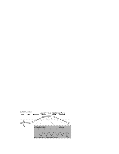
Figure 1: The physical system we solve. The equations describe the evolution of small scale perturbations embedded in an environment that is inhomogeneous on large scales and can have both a perturbation in the baryon density $\delta_{b}$ and in the radiation energy density $\delta_{r}$. The large scale inhomogeneities are the Horizon scale perturbations. The small scales are very short wavelength isothermal perturbations solved locally in a small region where the large scale can be considered uniform, or in other words, that the large scale flux is spatially constant. This approximation is possible because the small scale wavelengths considered are much smaller than the inhomogeneities affecting them.

We start by writing the equations of motion describing Newtonian isothermal fluctuations. The simplest equations describing matter fluctuations of scales much smaller than the horizon size and velocities much smaller than the speed of light are the Newtonian equations of motion, corrected to include the expansion of the universe. These are (see for example Kolb & Turner 1990):

$$0 = \dot{\rho}_{1}+3{\dot{a}\over a}\rho_{1}+{\dot{a}\over a}({\bf r}\cdot\nabla)\rho_{1}+\rho_{0}\nabla\cdot{\bf v}_{1}$$

$$0 = \dot{\bf v}_{1}+{\dot{a}\over a}{\bf v}_{1}+{\dot{a}\over a}({\bf r}\cdot\nabla){\bf v}_{1}+{v_{s}^{2}\over\rho_{0}}\nabla\rho_{1}+\nabla\phi_{1}-{\bf f}_{\rm rad}$$

$$0 = \nabla^{2}\phi_{1}-4\pi G\rho_{1},$$ (14)

where the various quantities have their usual meaning. Here $v_{s}$ is the isothermal speed of sound. The last term in the second equation is the force per unit mass acting on the baryonic fluid. It can be expressed with the help of the flux ${\bf H}$ observed in the baryonic rest frame and the opacity per unit mass $\kappa$. It can also be expressed with the radiation “velocity” ${\bf v}_{r}$ – the velocity with which the baryons need to move in order for them not to observe a net radiation flow, and a characteristic time $\tau_{e\gamma}$ for the transfer of momentum between the electron-proton fluid and the photons. If the angular dependence of the photon energy density distribution $\delta\rho_{r}(\theta,x)$ is expanded into Legendre polynomials:

$${\delta\rho_{r}(\theta,x,t)\over\rho_{r}(x,t)}=\sum_{\ell=0}^{\infty}\left(2\ell+1\right)P_{\ell}(\cos\theta)\sigma_{\ell}(x,t),$$ (15)

then the radiation “velocity” is given by $v_{r}\equiv\sigma_{1}/4$ and the flux observed in the baryon rest frame is $\left(\sigma_{1}-4v_{m}\right)c\rho_{r}$ with $v_{m}$ being the material velocity. Either way, the total radiative force per unit mass $f_{rad}$ can be written as:

$${\bf f}_{rad}={\bf H}\kappa={{\bf v}_{m}-{\bf v}_{r}\over\tau_{e\gamma}}.$$ (16)

We will work with the latter expression that uses the effective velocity of the radiation fluid $v_{r}$ as it is easier to work with when coupling the baryons to the radiation. For nonrelativistic velocities and Thomson scattering, the term can be written as:

$${\bf f}_{rad}={4\over 3}\sigma_{T}aT^{4}{{\bf v}_{m}-{\bf v}_{r}\over c}{n_{e}\over\rho_{b}}\equiv{{\bf v}_{m}-{\bf v}_{r}\over\tau_{e\gamma}}.$$ (17)

$n_{e}$ is the number of free electrons, $a$ denotes the radiation density constant, and $\sigma_{T}$ is the Thomson cross section.

Normally when linearised and Fourier transformed, this term which describes the radiation drag has a contribution only from the wave for which the linearized equations of motion are written. However, the contribution of waves of all scales should be taken into account if through the nonlinear interaction they produce a correction synchronised with the waves. When linearising, we find the following terms:

$${\bf f}_{rad}={{{\bf v}_{m}}_{1}-{{\bf v}_{r}}_{1}\over{\tau_{e\gamma}}_{0}}-{{{\bf v}_{m}}_{0}-{{\bf v}_{r}}_{0}\over{\tau_{e\gamma}}_{0}}{{\tau_{e\gamma}}_{1}\over{\tau_{e\gamma}}_{0}}.$$ (18)

The first term is responsible for the radiation drag due to the difference between the wave’s material velocity and the radiation “velocity”. The second term is due to the nonlinear effect that all other waves induce on this particular one through the change in the medium’s opacity and the shear between the material velocity and the effective radiation velocity of all other waves. The value of the large scale shear ${\bf v}_{m0}-{\bf v}_{r0}$ is the value at the region in which the small scale wave is solved for. The latter contribution is synchronised with the wave through the changes in the opacity. It is of second order and it should be integrated over time. Clearly, the contribution of waves oscillating at frequencies different than the particular wave averages to zero, thus, the only net contribution arise from waves that do not oscillate over the relevant integration time; that is to say, only the shear of the large scale waves contributes. If a wave oscillates $n$-times during the period, its net contribution will on average fall as $n^{-1}$. When integrated numerically in §5, the contribution of smaller scales is taken into account automatically and their contribution indeed falls with $\omega$.

The radiation field is not perturbed for optically thin, isothermal fluctuations. Consequently, ${{\bf v}_{r}}_{1}$ vanishes. If we define the large scale shear as:

$$\Delta{\bf v}_{0}\equiv{{\bf v}_{m}}_{0}-{{\bf v}_{r}}_{0},$$ (19)

and write

$${\tau_{e\gamma}}_{1}={\tau_{e\gamma}}_{0}\left(\alpha{\rho_{1}\over\rho_{0}}+\beta{T_{1}\over T_{0}}\right),$$ (20)

then the radiation term is:

$${\bf f}_{\rm rad}={{\bf v}_{1}\over{\tau_{e\gamma}}_{0}}+{\Delta{\bf v}_{0}\over{\tau_{e\gamma}}_{0}}{{\tau_{e\gamma}}_{1}\over{\tau_{e\gamma}}_{0}}\equiv{{\bf v}_{1}\over{\tau_{e\gamma}}_{0}}+{\Delta{\bf v}_{0}\over{\tau_{e\gamma}}_{0}}\left(\alpha{\rho_{1}\over\rho_{0}}+\beta{T_{1}\over T_{0}}\right).~{}~{}~{}$$ (21)

The second term does not vanish if the opacity is perturbed by the isothermal waves. By definition, the temperature isn’t perturbed and $T_{1}=0$. If however the opacity is a function of the density, then $\alpha\neq 0$ and a new term is added to the Newtonian equations of motion. The opacity is predominantly Thomson scattering, consequently, $\tau$ is proportional to the number of free electrons. The number of free electrons varies only during recombination. At this time $n_{e}$ is inversely proportional to the root of the density. To be more exact, the fraction of ionised protons at equilibrium $X_{eq}$ is given by Saha’s equation:

$${1-X_{eq}\over X_{eq}^{2}}={4\sqrt{2}\zeta(3)\over\sqrt{\pi}}\eta\left(T\over m_{e}\right)^{3/2}\exp(E_{ion}/T),$$ (22)

with the baryon to photon ratio $\eta$ being proportional to the density and $E_{ion}$ the ionisation energy of hydrogen. Through differentiation we find:

$$\alpha={\partial\ln X_{eq}\over\partial\ln\rho}=-{1-X_{eq}.\over 2-X_{eq}}$$ (23)

That is, before recombination commences, $X_{eq}$ is approximately unity and the parameter $\alpha$ vanishes. Afterwards it will grow in size and reach the asymptotic value of $-1/2$. Note that for the above equation to be valid, we need to assume that the time scale for ionisation equilibrium ($e+p\longleftrightarrow H+\gamma$) is shorter than the dynamic time scale. This implies that among other assumptions, the equations are valid only before freeze-in which takes place not too long after the advent of recombination. We have also neglected Helium ionisation and its influence on the density dependence of the opacity. However, the low abundance of Helium results with a much smaller effective $\alpha$, and together with the larger speed of sound, they both reduce the effect during the period of Helium recombination.

Define $\delta=\rho_{1}/\rho_{0}$ and spatially expand $\delta$, ${\bf v_{1}}$ and $\phi_{1}$ in Fourier integrals proportional to $\exp\left(-i{{\bf k}\cdot r/a(t)}\right)$. The result is:

$$0 = \dot{\delta}_{k}-{i{\bf k}\over a}\cdot{\bf v}_{k}$$

$$0 = a\dot{\bf v}_{k}+\dot{a}{\bf v}_{k}-i{\bf k}v_{s}^{2}\delta_{k}-i{\bf k}\phi_{k}+a{{\bf v}_{1}\over{\tau_{e\gamma}}_{0}}+\alpha a{\Delta{\bf v}_{0}\over{\tau_{e\gamma}}_{0}}\delta_{k}~{}~{}$$

$$0 = \phi_{k}+{4\pi G\rho_{0}\over k^{2}}a^{2}\delta_{k}.$$ (24)

The new phenomena discussed here arise from the introduction of the last term in the second equation. The term is proportional to the density perturbations (through opacity changes) and to the integrated large scale shear $\Delta v_{0}$ which varies in space. Even with the additional radiation term, the irrotational flow is still decoupled from the rotational part. On the other hand, the rotational part is affected from the irrotational one. This interesting effect can introduce a seed magnetic field from any isothermal fluctuation present, as is described in Shaviv & Levin (1998).

By taking the irrotational part of the second equation (through the dot product with ${\bf k}$), and using the first and last equations, we find that $\delta_{k}$ obeys the equation:

$$\ddot{\delta}_{k}+\left({2\dot{a}\over a}+{1\over\tau_{e\gamma}}\right)\hskip-1.0pt\dot{\delta}_{k}+\left({k^{2}v_{s}^{2}}-4\pi G\rho_{0}-i\alpha{\Delta\hskip-1.0pt{\bf v}_{0}\hskip-2.0pt\cdot\hskip-2.0pt{\bf k}\over\tau_{e\gamma}}\right)\hskip-1.0pt\delta_{k}\hskip-1.0pt=\hskip-1.0pt0$$

(25)

This equation (and its derivation) should be compared with the standard derivation of the equations describing isothermal waves when all nonlinear interactions are neglected (e.g., Coles and Lucchin, 1995). The solution of the linear equation consists of two modes. One describes a highly damped wave with a damping time scale of $\tau\sim\tau_{e\gamma}$. The other describes a frozen mode. Although the latter is formally unstable, the large radiation drag effectively reduces the growth rate to a value much smaller than the universe expansion rate.

4 Approximate Solution

The general solution to eq. 25 depends on the exact time dependence of $a$, $\dot{a}$, $\rho_{0}$, $\Delta v_{0}$ & $\tau_{e\gamma}$. We are however, interested in the evolution over the short period of decoupling, a period that is much smaller than the age of the Universe at the time. Moreover, we are particularly interested in circumstances were the growth rates are large, in fact, larger than the rate in which the various parameters change during recombination. This will allow us to assume that the above variables are quasi-static.

The system described by eq. 25 has five different time scales of which some depend on the wave number. The first two are the expansion age of the universe and the related Jeans timescale. For a flat matter dominated universe, the first is:

$$\tau_{\rm u}\equiv{3a\over 2\dot{a}},$$ (26)

while the second is:

$$\tau_{j}\equiv 1/\sqrt{4\pi G\rho_{0}}=\sqrt{3/2}\tau_{u}.$$ (27)

The last equivalence assumed a flat matter dominated universe. The third timescale is the isothermal oscillation time:

$$\tau_{o}^{-1}\equiv{|k|v_{s}}.$$ (28)

The fourth is the electron-photon relaxation time $\tau_{e\gamma}$ that describes how fast baryon and radiation exchange energy. The newly introduced timescale is the time associated with the radiation inhomogeneity:

$$\tau_{rad}^{-1}\equiv\sqrt{\alpha{\Delta{\bf v}_{0}\cdot{\bf k}/\tau_{e\gamma}}}.$$ (29)

We will assume here that the electron-photon relaxation time is much smaller than the universe’s expansion time scale. The reason being that when the timescale surpasses the expansion scale, the solution is in any case invalid because the timescale for establishing ionisation equilibrium becomes very long. The $\dot{a}/a$ term can therefore be neglected. The time scales themselves depend on the cosmic time as well, however, since we are interested in timescales shorter than both the expansion of the universe and the timescale for recombination of hydrogen, we can for simplicity assume them to be constant or quasi-stationary. In such a case, the equation’s solution is exponential with the roots:

$$r=-{1\over 2\tau_{e\gamma}}\pm\sqrt{{1\over 4\tau_{e\gamma}^{2}}-\left({1\over\tau_{o}^{2}}-{1\over\tau_{j}^{2}}-i{1\over\tau_{rad}^{2}}\right)}.$$ (30)

The waves’ growth rate is given by the real part of $r$, namely $\Re(r)$. It will be governed by the largest rate (or smallest time scale) in the system. The oscillatory behaviour is given by the Imaginary part – $\Im(r)$. For an optically thick universe with $\tau_{e\gamma}<\tau_{u}$, we find two general cases. The two cases and their various regions of $k$ in which the rates behave differently, are summarised in table 1 and exemplified in figure 2 where a few sample graphs of $\Re(r(k))$ are shown.

Case A: $\Delta v_{0}>v_{s}/\alpha$
Boundary between regions		Growth Rate: $\Re(r)$
		$k\ll k_{-\infty}$	$\Re(r)\approx{\tau_{e\gamma}/\tau_{j}^{2}}$
$\tau_{rad}^{2}=\tau_{j}\tau_{e\gamma}$	$k_{-\infty}\equiv{1\over\alpha\Delta{\bf v}_{0}\tau_{j}}$
		$k_{-\infty}\ll k\ll k_{0}$	$\Re(r)\approx\tau_{e\gamma}^{3}/\tau_{rad}^{4}=\tau_{e\gamma}\left(\alpha\Delta{\bf v}_{0}\cdot{\bf k}\right)^{2}$
$\tau_{e\gamma}=\tau_{rad}$	$k_{0}\equiv{1\over\alpha\Delta{\bf v}_{0}\tau_{e\gamma}}$
		$k_{0}\ll k\ll k_{\infty}$	$\Re(r)\approx\pm{1\over\sqrt{2}|\tau_{rad}|}=\pm\sqrt{{\alpha\over 2}{\Delta{\bf v}_{0}\cdot{\bf k}\over\tau_{e\gamma}}}$
$\tau_{rad}=\tau_{o}$	$k_{\infty}\equiv{\Delta{\bf v}_{0}\over v_{s}}{\alpha\over v_{s}\tau_{e\gamma}}$
		$k_{\infty}\ll k$	$\Re(r)\approx\tau_{o}/(2\tau_{rad}^{2})={\alpha\over 2}{\Delta{\bf v}_{0}\cdot\hat{\bf n}\over v_{s}}{1\over\tau_{e\gamma}}$
Case B: $\Delta v_{0}<v_{s}/\alpha$
Boundary between regions		Growth Rate: $\Re(r)$
		$k\ll k_{1}$	$\Re(r)\approx{\tau_{e\gamma}/\tau_{j}^{2}}$
$\tau_{o}=\tau_{u}$	$k_{1}\equiv{1/(\tau_{u}v_{s})}$
		$k_{1}\ll k\ll k_{2}$	$\Re(r)\approx-\tau_{e\gamma}/\tau_{o}^{2}=-\tau_{e\gamma}v_{s}^{2}k^{2}$
$\tau_{e\gamma}=\tau_{o}$	$k_{2}\equiv{1/(\tau_{e\gamma}v_{s})}$
		$k_{2}\ll k$	$\Re(r)\approx-1/2\tau_{e\gamma}$

Table 1: The growth rate of the small scale waves for various wavelengths under the two relevant cases of ${\Delta v_{0}}>v_{s}/\alpha$ and ${\Delta v_{0}}<v_{s}/\alpha$, with $\tau_{e\gamma}<\tau_{u}$ ( i.e., as long as the universe is optically thick). Note that only if $\Re(r)>\tau_{u}^{-1}$ is the solution appropriate. Otherwise, instead of an exponential solution, the system will evolve through a power law behaviour with a typical growth scale of $\tau\sim\Re(r)$.

When analysing eq. 30, one finds that it admits two general forms of behaviour depending on whether $\Delta v_{0}$ is smaller or larger than $v_{s}/\alpha$. The main difference between the two cases is that large $k$ waves in the former case are damped while in the latter they are unstable and amplify. More specifically, one has:

Case A: $\Delta v_{0}<v_{s}/\alpha$
When the shear velocity between the radiation and baryon fluid is smaller than the critical value, the shear cannot overcome the radiation drag. Even though the quantitative analysis may change, the general behaviour is the one found when the shear velocity is altogether neglected. That is to say, long wavelengths for which $\tau_{o}>\tau_{u}$ are frozen in the plasma. Although they do have a positive growth rate, it is small when compared with the growth rate of the horizon. Waves with smaller wavelengths for which $\tau_{o}<\tau_{u}$ are damped, and when $\tau_{e\gamma}\sim\tau_{o}$, the damping rate is saturated at its asymptotic value of $1/2\tau_{e\gamma}$.

Case B: $\Delta v_{0}>v_{s}/\alpha$
The behaviour of the system is radically different when the large scale shear velocity is larger than the critical value. At large wavelengths, the waves are still frozen in and the behaviour is the same as in the previous case. On the other hand, at shorter wavelengths the waves’ growth rate is dominated by $\tau_{rad}$. Instead of being damped or frozen-in, the waves can in this case be unstable. The growth rate of waves propagating in the direction of the shear increases with $k$ and it saturates at small wavelengths when acoustic oscillations become important. The maximum or asymptotic growth rate is obtained for values of $k$ larger than:

$$k_{\infty}={\Delta{\bf v}_{0}\over v_{s}}{\alpha\over v_{s}\tau_{e\gamma}},$$ (31)

i.e., for scales smaller than the Jeans scale by a factor of order ${\tau_{u}/\tau_{e\gamma}}$. The typical values of $\tau_{u}/\tau_{e\gamma}$ when the rate is large are of order 10, implying that the typical scales would be 10 times smaller than the Jeans scale. The maximum growth rate is then given by:

$$\Re(r)\approx\tau_{o}/(2\tau_{rad}^{2})={\alpha\over 2}{\Delta{\bf v}_{0}\cdot\hat{\bf n}\over v_{s}}{1\over\tau_{e\gamma}}.$$ (32)

It is now evident why isothermal waves are crucial. The speed of sound $v_{s}$ in isothermal waves is much smaller than the speed of light, therefore, the typical shears that cause nonlinear interactions are of order ${\cal O}(v_{s}/c)$ and not ${\cal O}(1)$! An appreciable nonlinear effect can take place already at a dimensionless amplitude of $\delta\rho/\rho\sim 10^{-5}$ or $10^{-4}$!

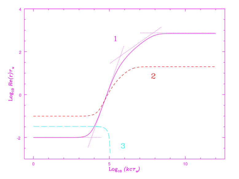
Figure 2: The growth rate as a function of the wave number depicted for three examples. In all three examples shown $v_{s}=10^{-5}c$ and $\alpha=1/2$. In example 1: $\Delta v_{0}=3\times 10^{-4}$ and $\tau_{e\gamma}=0.01\tau_{u}$, in example 2: $\Delta v_{0}=1\times 10^{-4}$ and $\tau_{e\gamma}=0.1\tau_{u}$, while in example 3: $\Delta v_{0}=1\times 10^{-5}$ and $\tau_{e\gamma}=1/30\tau_{u}$. The first two examples correspond to case A of table 1 while the third example for which $\delta v_{0}<v_{s}/\alpha$ corresponds to case B in the table. Only in the former two cases do we find that the growth rate is increased tremendously for large values of $k$. The curve of example 1 has the approximate behaviour corresponding to the four different regions of case A marked with small dotted lines in addition to the exact value of the root. In the four different regions, we have $k\propto const,k^{2},k^{1/2},const$. They do not exist in example 3, and while they do exist in the second example, the behaviour is not as clear as in the first one.

We are interested in the integrated effect of the growth rate in the time interval between a given $t_{0}$ and a given later time $t_{1}$. Hence, we define the following growth parameter:

$$G(k,\hat{\bf n})=\int_{t_{0}}^{t_{1}}\Re(r(k,\hat{\bf n}))dt.$$ (33)

If the rate given by eq. 32 is larger than all other inverse timescales of the system on which the value of the rate can change (i.e., both the expansion and the recombination timescales) then the growth factor of the isothermal waves is approximately given by:

$${\delta_{t_{1}}(k,\hat{\bf n})\over\delta_{t_{0}}}\approx\exp(G(k,\hat{\bf n})).$$ (34)

The recombination time $\Delta t\equiv t_{1}-t_{0}$ is the shortest timescale on which the growth rate changes. As a consequence, the condition for the approximation to hold can be written as $\Re(r)\gg\Delta t^{-1}$, and it can be translated through eq. 33 to $G\gg 1$.

We proceed to investigate the rate of growth in two ways:

• The nonlinear growth rate equation (eq. 34) is averaged over the distribution of perturbation amplitudes and direction of motion in order to get the average growth of the amplitude of the waves.

• We explore systems that reach nonlinear amplitudes by examining the volume fraction that does develop nonlinearities and the possible effects triggered by these nonlinear regions.

4.1 Average Growth

We now proceed to estimate the average growth of amplitude of small scale waves for which $k\ga k_{\infty}$. Although the physical scale is small enough not to be directly detectable in the near future, these modes have the fastest growth rate and are therefore most interesting.

The averaging procedure of the amplification described by equation 34 should be divided into two separate averages over two distributions. First, the expression should be averaged over the various possible propagation directions since unlike the nonlinear case, the dispersion relation is now a function of the direction of ${\bf k}$ (with respect to the direction of the large scale shear) and not only its absolute value. Second, the growth function is found for a given local value of the shear, however, it is certainly not linear in its amplitude and one should therefore average over the distribution of large scale shears.

We first average expression 34 over the $4\pi$ possible directions of $\hat{\bf n}$ (the direction of ${\bf k}$) while keeping in mind that $G$ is linearly proportional $\hat{\bf n}\cdot\hat{\bf n}_{0}$. We get:

$$\left\langle{\delta_{t_{1}}(k,\hat{\bf n})\over\delta_{t_{0}}}\right\rangle_{\hat{\bf n}}=\int d\hat{\bf n}{\delta_{t_{1}}(\hat{\bf n})\over\delta_{t_{0}}}$$ (35)

$$\phantom{\left\langle{\delta_{t_{1}}(k,\hat{\bf n})\over\delta_{t_{0}}}\right\rangle_{\hat{\bf n}}}=\int d\hat{\bf n}\exp(G_{\infty}(k)(\hat{\bf n}\cdot\hat{\bf n}_{0}))={\sinh(G_{\infty}(k))\over G_{\infty}(k)}$$

with $G_{\infty}(k)=G(k,\hat{\bf n}=\hat{\bf n}_{0})$, i.e., its maximum value.

Next, we proceed to average over the distribution of shears $\Delta{\bf v}_{0}$. This distribution will clearly depend on the form of the density distribution. The natural choice for the latter is a Gaussian distribution. Although it does not necessarily have to be the case, it is the theoretically most reasonable distribution expected for the density fluctuations. The distribution of the absolute value of the shears is similar in form to the distribution of the absolute velocities calculated from density perturbations in large scale structure (e.g. Coles and Lucchin §18.3), that is, if the distribution for the density fluctuations is Gaussian then it will be Guassian for the components of the shear vector in each axis, and the distribution for the absolute value will be given by a Maxwellian distribution. If the root mean square of $G_{\infty}$ is $G_{rms}$, the distribution itself is:

$$P(G_{\infty})=\sqrt{54\over\pi}{G_{\infty}^{2}\over G_{rms}^{3}}\exp\left[-{3\over 2}\left(G_{\infty}\over G_{rms}\right)^{2}\right].$$ (36)

The average perturbation growth factor is therefore:

$$\left\langle{\delta_{t_{1}}\over\delta_{t_{0}}}\right\rangle_{all}$$ (37)

$$~{}~{}~{}~{}~{}=\int_{0}^{\infty}\sqrt{54\over\pi}{G_{\infty}^{2}\over G_{rms}^{3}}\exp\left[-{3\over 2}\left(G_{\infty}\over G_{rms}\right)^{2}\right]{\sinh(G_{\infty})\over G_{\infty}}dG_{\infty}$$

$$~{}~{}~{}~{}~{}=\exp\left(G_{rms}^{2}\over 6\right)\equiv{\cal A}(G_{rms}).$$

The function ${\cal A}(G_{rms})$ describes the amplification factor of the fluctuations. Clearly, for $G_{rms}$ much less than or of order unity, the effect is small or negligible. Moreover, the numerical values obtained, such as a 10% increase for $G=1$, are only approximate since the required condition $G\gg 1$ for the validity of eq. 34 is not fulfilled. Nonetheless, already at $G_{rms}=5$, small scale isothermal fluctuations will amplify by almost 2 orders of magnitude. They will grow by 5 orders of magnitude for $G_{rms}=8$ and for $G_{rms}=12$ the growth will be a staggering 10 orders of magnitude. Note that if the growth is saturated when the amplitude reaches nonlinearity then the average growth is meaningful only if the amplified amplitude is less than unity. Moreover, unlike the case when $G_{rms}\sim 1$, the solution here is much more accurate because regions that contribute the most to the growth are those in the high $G_{\infty}$ tail, where the approximate solution is valid. For example, the average growth when $G_{rms}=8$ is of 5 orders of magnitude and the main contribution originates from $G_{\infty}\sim\ln(10^{5})\approx 11.5\gg 1$.

Also worth mentioning is that in the averaging procedure over the fluctuation distribution, we are essentially averaging an exponential function $\sim\exp(G_{\infty})$; thus, if the distribution for the amplitudes does not fall fast enough for large values of $G_{\infty}$ (which is proportional to $\delta\rho/\rho$), the averaging integral diverges. Such a divergence occurs if the high $\delta\rho/\rho$ tail is for example a power law. The implication is that there will always be a finite volume (i.e., volumes that are not exponentially small) where nonlinearity can be reached if the distribution has a wide tail. A wide tail can in this case be any distribution with a power law tail or even a distribution with an exponential tail, provided the tail of the distribution is in the form $\propto\exp(-G_{\infty}/G_{0})$ with $G_{0}>1$.

4.2 The nonlinear regions

The large exponential growth associated with small regions where the shear is large, is of high importance. In these regions that are small for a modest value for $G_{rms}$, the growth may be large enough as to amplify waves out of the linear regime and let the nonlinear evolution of these wave commence. Consequently, it is interesting to estimate what fraction of space will actually be filled with nonlinear waves by the end of recombination.

The largest growth factor in a given region is given by $\sim\exp(G_{\infty})$. Thus, if the typical small scale fluctuation amplitude before amplification is initially $\delta_{0}$, then only if $\delta_{0}\exp(G_{\infty})\ga 1$ will there be waves that grow out of linearity, i.e., only if $G_{\infty}\ga-\ln\delta_{0}$. If the density fluctuations are Gaussian, the distribution of growth factors $G_{\infty}$ is Maxwellian and given by eq. 36. The fraction of space in which there are waves that reach nonlinearity is then given by

$${\cal F}(\delta_{0},G_{rms})=\hskip-2.0pt\int_{-\ln\delta_{0}}^{\infty}\sqrt{54\over\pi}{G_{\infty}^{2}\over G_{rms}^{3}}\exp\left[-{3\over 2}\left(G_{\infty}\over G_{rms}\right)^{2}\right]dG_{\infty}$$

$$~{}~{}={\rm erfc}\left(-{3\over 2}{\ln\delta_{0}\over G_{rms}}\right)-\sqrt{6\over\pi}\exp\left(-{3\over 2}\left(\ln\delta_{0}\over G_{rms}\right)^{2}\right){\ln\delta_{0}\over G_{rms}}.~{}$$ (38)

Here erfc denotes the complementary error function. The function $\cal F$ is plotted in figure 3. As an example, for $G_{rms}\sim 5$, $\delta_{0}$ should be roughly $10^{-4}$ to have 1% of the volume reach nonlinearity.

If we could observationally detect all the regions in the background microwave sky that reach nonlinearity (see e.g. §5) then the absolute number of regions showing nonlinearity will be given by the fraction that does develop it multiplied by the total number of statistically independent regions. The latter number is roughly $4\pi\ell^{2}$ with $\ell$ the multipole order corresponding to the typical shear producing wavelengths. By taking a co-moving $k\sim 0.1Mpc^{-1}$ as the typical correlation length for the shear producing zones (see e.g. §5 or fig. 7) we get:

$$\ell\approx(6000~{}h^{-1}Mpc)k\sim 1000,$$ (39)

namely, to get a statistically significant number of regions, one must have:

$${\cal F}(\delta_{0},G_{rms})\gg{1\over 4\pi\ell^{2}}\sim 10^{-7}.$$ (40)

Evidently, for our example of $G\approx 5$, any initial isothermal perturbations that has $\delta_{0}\ga 10^{-6}$ is theoretically detectable and will produce at least 100 different nonlinear regions. If the primordial spectrum of fluctuations is isothermal and flat, and the expectation for $\delta_{0}$ is $\sim 10^{-4}$ then for any $G_{rms}>3$ one should in future be able to detect the effect. For $G\ga 10$ more than 50% of the universe reaches nonlinearity at $z\sim 1000$. In the case where the isothermal wave amplitude has the smallest plausible value, namely when the primordial spectrum is flat and adiabatic and the Press-Vishniac (1979) effect produces isothermal waves with an amplitude $\delta_{0}\sim 10^{10}-10^{-8}$, the effect will be detectable for any $G_{rms}\ga 7.5$.

Figure 3: The fraction of regions that reach nonlinearity – ${\cal F}(\delta_{0},G_{rms})$ as a function of $Log_{10}(1/\delta_{0})/G_{rms}$. Any fraction less than $\sim 10^{-6}$ will be theoretically impossible to detect and correlate with gradients in the CMBR at a $3\sigma$ level, as there are only about $10^{7}$ statistically independent regions for which the shear is substantially different and uncorrelated.

5 Estimating the effect in actual cosmological scenarios

The largest attainable growth parameter is roughly:

$$G_{\infty}\approx{\alpha\over 2}{{\Delta v_{0}}\over v_{s}}{\Delta t\over\tau_{e\gamma}}.$$ (41)

where $\Delta t$ is the approximate duration of decoupling. $v_{s}$ is the isothermal sound speed which at recombination is about 4.8 orders of magnitude less than the speed of light. Therefore, when recombination commences and $\tau_{e\gamma}\sim 10^{-2}\tau_{u}$ (for an approximate duration of $\Delta T\approx 10^{-1}\tau_{u}$), the shear velocity should be about $3\times 10^{-5}c$ to get a 2 order of magnitude increase and $6\times 10^{-5}c$ to get as much as a 10 orders of magnitude increase. As recombination continues, the shear increases while $1/\tau_{e\gamma}$ and the optical depth decrease roughly by the same factor, such that the rate of growth is effectively unchanged during this period, even though the opacity changes by more than two orders of magnitude.

The interesting question that will ultimately determine the fate of the small scale fluctuations is therefore a quantitative one – what is the exact value (i.e. the exact r.m.s.) of the shear exerted by large scales and what is the integrated rate equal to?

To answer the quantitative question, a numerical simulation for the behaviour of the large scale modes was carried out. The numerical code is a modification of the COSMICS code developed by Bertschinger and Ma. The code was used to integrate the linearised equations of general relativity, matter and radiation in the synchronous guage, and subsequently normalize the power spectra to the COBE measured quadrupole moment. A description of the equations solved and the numerical algorithm used can be found in Bertschinger (1995) and Ma & Bertschinger (1997). With the modification, the maximum growth rate given by eq. 32 is calculated and integrated to give the growth parameter.

The evolution of each co-moving large scale wave vector $k$ is followed over the course of the particular scenario’s cosmological history. For each $k$ integrated, the code calculates the evolution of the wave amplitude of the various species in the primordial soup, including among other, the angular moments of the photon distribution $\Delta_{\ell}(k,t)$. These are to be precise, the Fourier and Legendre decomposition of the photon brightness temperature perturbation $\Delta({\bf x},{\bf{\hat{n}}},t)\equiv\Delta T/T$ of the photons traveling in the direction of ${\bf\hat{n}}$; more specifically, they are defined through:

$$\Delta({\bf x},{\bf{\hat{n}}},t)\hskip-1.0pt=\hskip-3.0pt\int d^{3}ke^{i{\bf k}\cdot{\bf x}}\sum_{\ell=0}^{\infty}(-1)^{\ell}(2\ell+1)\Delta_{\ell}({\bf k},t)P_{\ell}({\bf\hat{k}}\cdot{\bf\hat{n}}).~{}$$ (42)

The program also integrates the appropriate unnormalized growth factor:

$$g_{\infty}(k,t)=\int_{0}^{t}{\alpha\over 2}{{\Delta v_{0}}\over v_{s}}{dt\over\tau_{e\gamma}},$$ (43)

where $\Delta v_{0}$ is the unnormalized shear.

To normalize both $\Delta_{\ell}(k,t)$ and $g_{\infty}(k,t)$, one should take into account the original, primordial power spectrum $P(k)=Ak^{4-n}$. When $n=1$ the power index corresponds to a flat Harrison-Zel’dovich power spectrum for which the total power per decade is constant. We normalize the spectrum to fit the measured COBE quadrupole moment. This is achieved through the separation of the angular correlation function $C(\theta)$ into its moments:

$$C(\theta)=\sum_{\ell}{2\ell+1\over 4\pi}C_{\ell}P_{\ell}(\cos\theta),$$ (44)

with $P_{\ell}$ the $\ell$’th Legendre polynomial, and writing the moments as a function of the normalized photon power distribution functions:

$$C_{\ell}=4\pi\int d^{3}kP(k)\Delta_{\ell}^{2}(k).$$ (45)

The quadrupole moment is related to the second moment $C_{2}$ of the angular correlation function by the definition:

$$Q_{rms-PS}\equiv T_{0}\left(5C_{2}\over 4\pi\right)^{1/2},$$ (46)

through which the constant $A$ of the power spectrum can be normalised. The value used for the quadrupole moment is $Q_{rms-PS}=18\mu K$ . The r.m.s. of $G_{\infty}$ can then be related to the unnormalized growth rate (eq. 43) through the expression:

$$G_{rms}^{2}=\int d^{3}kP(k)g_{\infty}^{2}(k).$$ (47)

A few cosmological scenarios were checked, all of which correspond to flat universes. Typical results are summarised in figures 4-7. In figure 4 we find the various physical parameters that affect the large scale shear. Figures 5 and 6 depict the unnormalized growth rate and its integrated value (the growth parameter) as a function of time for several co-moving wavenumbers in a standard CDM model (run 1). The last figure describes the integrated growth parameter as a function of co-moving wavenumber for two scenarios - a standard CDM and a mixed Hot-Cold dark matter scenario. We find that most of the contribution comes from a co-moving $k\sim 0.1~{}Mpc^{-1}$ but a significant contribution arises from scales that are smaller or larger by as much as an order of magnitude (or even more in the case of CDM).

The scenarios simulated are summarised in table 2. We find that the typical r.m.s. of $G_{\infty}$ varies from slightly less than unity to more than 5, i.e., the average growth of the small scale isothermal waves in flat cosmologies can range from 10% to 2 orders of magnitude, depending on the particular scenario.

Run	Model	$\Omega_{b}$	$\Omega_{c}$	$\Omega_{\Lambda}$	$\Omega_{\nu}$	$n$	$G_{rms}$
1	std. CDM	.05	.95	–	–	1	5.1
2	std. CDM	.02	.98	–	–	1	4.7
3	tilted. CDM	.05	.95	–	–	.9	4.2
4	Mixed HCDM	.05	.75	–	.2	1	0.9
5	$\Lambda$-CDM	.05	.55	.4	–	1	2.8

Table 2: Summary of the numerical results. All models are flat (curvature free) universes with a Hubble constant of $H_{0}=66km~{}sec^{-1}Mpc^{-1}$ and with adiabatic initial perturbations.

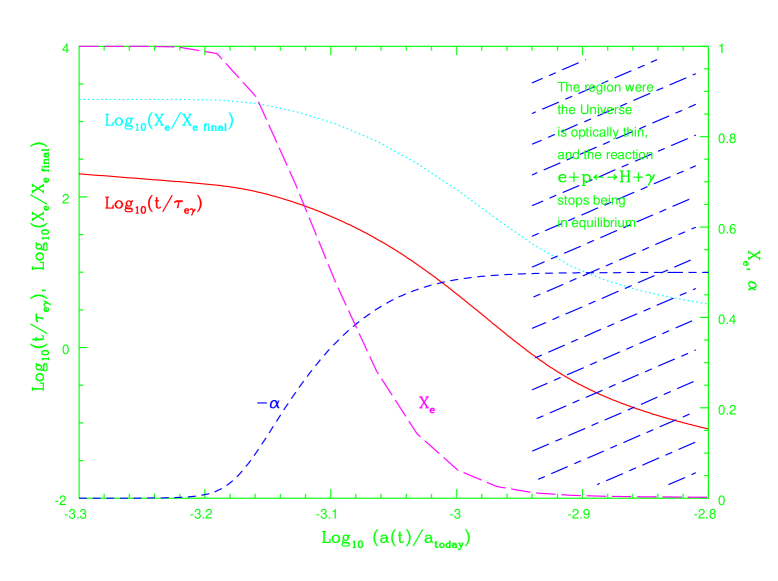
Figure 4: The various physical variables that affect the net shear in the system and its effect on small scales as a function of expansion radius of the universe for a sCDM model with $H_{0}=66~{}km~{}s^{-1}~{}Mpc^{-1}$ and $\Omega_{b}=0.05$. The variables are $\alpha=\partial\log X_{e}/\partial\log\rho$ which directly affects the strength of the force induced on small scales, $X_{e}$, the number of free electrons to which the total force is proportional, $t/\tau_{e\gamma}$ gives the mean free path of an electron in the photon “fluid” to horizon scale ratio, while $X_{e}/X_{e~{}final}$ is the ionisation to residual ionisation ratio. If it is much greater than unity, the reaction $e+p\longleftrightarrow H+\gamma$ is still in equilibrium and the solution is valid .

Figure 5: The (unnormalized) evolution of the instability growth rate $g_{\infty}(k,t)$ as a function of the universe expansion scale for five different wave numbers; namely, the contribution to the large scale shear from various wavelengths during the time of recombination. For sub-Horizon scales which are not too small, waves with larger $k$ oscillate more times during recombination and cancel out some of their contribution. However, when $k$ is increased further, the optical depth corresponding to one wavelength falls below unity and the radiation fluid and baryon fluid stop oscillating synchronously. As the baryon fluid loses its radiation support, its oscillations decreases, as can be seen in the figure. As a consequence, the contribution from large wavenumbers does not fall as fast as $1/k$, as is evident in fig. 8. The scenario is a standard CDM with $H_{0}=66~{}km~{}s^{-1}~{}Mpc^{-1}$, $\Omega_{b}=0.05$ and a flat adiabatic primordial spectrum (run 1).

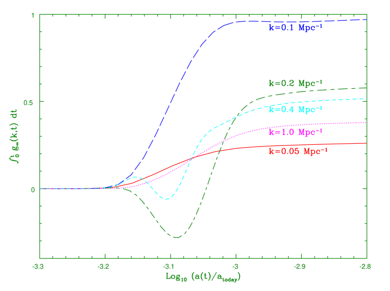
Figure 6: The same as the previous figure except that plotted are the time integrated growth rates.

Figure 7: The (unnormalized) integrated growth rate as a function the co-moving wavenumber $k$ for two cases. One is the standard CDM (run 1) while the other is a mixed Hot-Cold dark matter (run 4), with parameters given in table 2.

6 Can early small scale structure formation be measured?

We have found that small scale perturbations can under certain conditions be enormously amplified. The strong enhancement of particular waves leads to the following questions: First, if the required conditions do prevail and the amplification factor is more than enough to drive the perturbation out of the linear regime, at what point will the growth process stop? Second, if this process did in fact take place early in our universe, could it have left a mark on the CMBR that is detectable today? And third, could the process have had other implications on structure formation in the early universe?

It is difficult to precisely estimate when the growth saturates. The simplest estimate to when the growth process ceases is as the wave reaches the nonlinear regime, a point at which our linear treatment breaks down anyway. Clearly, when $\delta\rho/\rho$ is of order unity, the different speeds of sound at different parts of the wave can create shocks that will dissipate the waves’ acoustic energy into thermal energy. When $\delta\rho/\rho\sim 1$, the acoustic energy of isothermal waves is of order the thermal energy of the gas alone (In adiabatic waves the energy is of order the thermal energy of the gas and radiation). At the time of recombination, the heat capacity is very large because a large amount of energy is needed to reionise the Hydrogen. Thus, after recombination, when the temperature is of order but less than the recombination temperature $T\la T_{rec}\approx 0.26eV$, injecting an amount of order the thermal energy of the plasma will ionise at most only $\sim T_{rec}/E_{ion}\approx 0.26eV/13.6eV\approx 1/50$ of the Hydrogen atoms. The free electrons released by ionization rescatter photons and leave a mark in the CMBR.

Heating the plasma back to the recombination temperature implies that the plasma and the microwave background are not in equilibrium anymore. The plasma consequently upsets the Planck distribution of the radiation through the number conserving Compton scattering process. The process is evident from Kompaneets’ equation (1957) and its cosmological application by Sunyaev and Zel’dovich (1969). The dimensionless parameter describing the importance of the effect is the parameter $y$ defined as:

$$y={k\left<T_{e}\right>\over m_{e}c^{2}}\int^{t}\sigma_{T}n_{e}cdt,$$ (48)

with standard notations. $n_{e}$ denotes the number of free electrons. The analysis of the COBE data revealed no deviation from a Planckian spectrum and set a limit of (Fixsen et al. 1996):

$$y\la 1.5\times 10^{-5}~{}~{}~{}(95\%CL).$$ (49)

If the fraction of ionised electrons increases to $\iota_{e}\sim 1/50$, and the temperature $T$ increases to $\tau T$ with $\tau\sim 1$, one can show that the resulting $y$ parameter should be of order (e.g. Peebles, 1993):

$$y\sim 2\times 10^{-11}(\tau-1)(1+z)^{5/2}h\Omega_{b}\Omega^{-1/2}\iota_{e}.$$ (50)

with $z\sim 1000$ at recombination. Thus,

$$y_{max}\sim 4\times 10^{-6}h_{0.75}{\Omega_{b}}_{0.05}\Omega^{-1/2}.$$ (51)

If through the appropriate nonlinear treatment it would be found that the kinetic energy of the saturated waves is larger than the thermal energy then the energy, disspated is larger and $y_{max}$ should be increased correspondingly. If on the other hand the dissipation is found to take place on smaller time scales than the universe’s age at the time, $\tau-1$ is smaller and it reduces $y_{max}$. The actual values cannot be found from our linear analysis.

The aforementioned value for the $y$ parameter is however only in regions (and directions in the sky) where the gradient at recombination was large enough to have isothermal waves reach saturation. The average $y$ will be smaller and given by:

$$y_{avr}=y_{max}{\cal F}\left(\log\delta_{0}\over\log G\right).$$ (52)

Unless the fraction $\cal F$ of the sky that reaches nonlinearity is of order unity, the $y_{avr}$ is too small to be detectable by present means. Nevertheless, investigations that correlate $y$ with the gradients in future sub-degree maps will be able to detect smaller values for $y$.

If the observations rule out the existence of such structure then the theory imposes strict limits on the cosmological parameters, including the fact that the fluctuation distribution function does not have a power law tail. However, it can predict black-body deformations correlated with the CMBR gradients (i.e., a specific correlation). If indeed this is the case, it will be proven as the origin for small scale structure, and it could be used for setting strict limits on cosmological parameters.

7 Exotic Possibilities

More exotic possibilities for the fate of the nonlinear regions rely on the fact that the sub-Jeans sized objects formed through the radiative instability during recombination can later on gravitationally collapse. The typical wave numbers that experience the large amplification are those with a wavelength larger than the Jeans scale by at least an order of magnitude. If they exist in the linear regime they are unstable and collapse when $z\sim 10$, however, these wave lengthes are already nonlinear at $z\sim 1000$ and may easily collide and collapse long before their linear cousins will. Compact objects of order of the Jeans scale can therefore form and collapse at very high redshifts $10\la z\la 1000$. What will the fate of these objects be? They might collapse into massive Black holes, they can also burn and release a few$\times 10^{-5}$ of their energy while doing so (Bond et al. 1984). These nonlinearities may perhaps form globular cluster like clusters or maybe even seeds for AGN engines.

Another possibility is that the nonlinear objects form structure on larger scales through the large energy they release and a chain reaction of explosions that they ignite (Ostriker & Cowie, 1981), they can then prompt the collapse of galaxies in the expanding shells and form voids. Although the peculiar velocity and the $y$-distortion prediced for the simplest of these models are both too high (Levin, Freese & Spergel, 1992), the inclusion of continuous or multi-cycled detonation waves in the explosion model can lead to large voids with a diameter larger than 10 Mpc, a peculiar velocity of roughly $100~{}km~{}sec^{-1}$ and a $y$-distortion less than the limit set by COBE (Miranda & Opher, 1997). If these explosions can indeed be ignited, only a very small fraction of the universe needs to reach the nonlinear regime by the end of recombination in order to have dramatic effects on the formation of large scale structure.

8 Feedback on larger scales

The next question to address is whether the effect can also affect the large scales. Since energy is conserved, large scales will be affected if the energy transferred to the smaller scales is comparable to the original energy in the large scales. The energy per unit mass in the large scale waves is roughly given by $(\delta\rho_{ad}/\rho)^{2}v_{(a)}^{2}/2$ while the energy per unit mass in the small scale isothermal waves is roughly $(\delta\rho_{iso}/\rho)^{2}v_{(i)}^{2}/2$. Inspection of eq. 12 reveals that when the small isothermal waves have a dimensionless amplitude of order unity over a large fraction of the universe and $G_{rms}\sim 1$, the energy content in both types of waves is comparable. A significant fraction of the energy in the large scales can therefore be transferred to the small scales.

Apparently, an exact treatment is beyond the scope of the linear analysis developed here and the unknown nonlinear physics can at most be phenomenalised using few parameters and a simple demonstrative model.

Using the terminology and approximations of §2, one can express the original energy per unit mass in the large scales as $A_{l}^{2}G_{rms}^{2}\times v_{(i)}^{2}/2$. Under the approximation of §2, we have $A_{l}=4$, however, for optically thin large scale waves the energy in the waves is different and $A_{l}$ can change. The energy in the isothermal waves is $A_{s}^{2}\times v_{(i)}^{2}/2$ and the energy growth rate is $2G_{rms}A_{s}^{2}/\Delta t\times v_{(i)}^{2}/2$.

Next, we assume the energy damping rate of the small scale waves to be of the form:

$$\left.{dE\over dt}\right|_{damping}\equiv{A_{d}\over\Delta t}A_{s}^{\epsilon}\times v_{(i)}^{2}/2.$$ (53)

$\Delta t$ is the duration of recombination. $A_{d}$ and $\epsilon$ are parameters that represent the unknown physics. Both parameters can depend on the wavelength of the unstable isothermal waves. $A_{d}$ should be of order unity for waves with a period of $\sim\Delta t$, but otherwise unknown. The power $\epsilon$ with which the damping depends on the amplitude of the isothermal wave is also unknown but should satisfy $\epsilon>2$ if it is characterised with only one power index and if it is to be more important on the nonlinear scales than on the linear ones.

If the value of $G_{rms}$ before the instability commences is large enough then a large fraction of the volume leaves the nonlinear regime. The critical value for this to take place is

$$G_{rms}\ga-\ln(\delta\rho_{iso}/\rho).$$ (54)

The simplest simplifying assumption is that the isothermal waves will saturate at a level where the energy growth rate is equal to the dissipation rate. The small scale amplitude $A_{s}$ will then be given by

$$A_{s}=\left(G_{rms}\over A_{d}\right)^{1\over\epsilon-2}.$$ (55)

Compare now the energy in the large scales with the total energy that can be dissipated. When the latter energy is larger, all the energy in the large scales can be dissipated. The condition for it to take place is:

$$\left\{\begin{array}[]{c l}G_{rms}\la 2^{\epsilon-2}A_{d}^{2/(4-\epsilon)}A_{l}^{2/(4-\epsilon)}&{\rm for}~{}\epsilon<2~{}{\rm or}~{}\epsilon>4\\ G_{rms}\ga 2^{\epsilon-2}A_{d}^{2/(4-\epsilon)}A_{l}^{2/(4-\epsilon)}&{\rm for}~{}2<\epsilon<4\end{array}\right.$$ (56)

When $2<\epsilon<4$, an initial value of $G_{rms}$ that satisfies the above condition will imply that the amplitude of the large scale fluctuation can be reduced until $G_{rms}$ does not comply with the above condition. For other values of $\epsilon$, the initial value of $G_{rms}$ must be smaller than a critical value in order to satisfy the above condition, in which case, the large scale amplitude will apparently be reduced arbitrarily. In fact, $G_{rms}$ continues to decrease until the shear drops below the critical value separating between the two cases, at which moment the instability turns off. Since $\tau_{e\gamma}\sim 1$ at the end of recombination (see e.g. figure 4), the switching off will take place at $G_{rms}\sim 1$. To summarise, two possibilities for the damping of large scale waves seem to exist depending on the power $\epsilon$ relating the dependance of the damping rate with the amplitude of the isothermal wave. In the first case, any $G_{rms}$ larger than roughly the critical value given by eq. 56 will be reduced to a value of order of critical value provided that it satisfied eq. 54 as well. In the second case, any $G_{rms}$ which satisfies both eq. 56 and eq. 54, will be reduced to $G_{rms}\sim 1$.

As an elucidation, one can numerically solve a simplified toy model for the process. The transfer of energy from the large scales into the small scales and then the dissipation by small scale nonlinearities can be simplified and described with the two differential equations:

$${d\over dt}\left(A_{l}^{2}G_{rms}(t)^{2}\right) = -{2G_{rms}(t)\over\Delta T}A_{s}(t)^{2}$$ (57)

$${d\over dt}\left(A_{s}(t)^{2}\right) = +{2G_{rms}(t)\over\Delta T}A_{s}(t)^{2}-{A_{d}\over\Delta T}A_{s}(t)^{\epsilon}.$$

Figs. 8a & 8b describe the numerical results for the integration of the two differential equations when $\epsilon=3$, $A_{d}=1$, $A_{l}=4$, for initial fluctuations of $\delta\rho_{iso}/\rho=10^{-5}$ and different initial values of $G_{rms}$. By comparing to the numerical results to eq. 56, it is clear that the analytical estimate is an over simplification of the differential equations, which too are a simplification of the real physics. Nevertheless, the main conclusion is that for a large range of an initial large-scale amplitudes, it is possible to have almost all the energy dissipated into smaller scales and subsequently have it dissipated through nonlinear processes. The large scales then reach their natural lower limit – the value for which the large scale shear switches off the instability.

Figure 8: The two panels represent the results of the numerical integration of the two approximate differential equations describing the evolution of the energy in the large scales ($A_{l}^{2}G_{rms}^{2}\times v_{(i)}^{2}/2$) and in the small scales ($A_{s}^{2}\times v_{(i)}^{2}/2$). The initial small scale amplitude before the instability takes place is $A_{s}(t=0)=10^{-5}$. Also, $\epsilon=3$, $A_{d}=1$ and $A_{l}=4$. The evolution of $A_{s}(t)$ and $G_{rms}(t)$ is depicted in panel a for various initial values of $G_{rms}$. Note that only part of the recombination period $\{0,\Delta t\}$ is shown. The same cases are drawn with the same line type in both parts. Panel b depicts the final values at the end of recombination – $A_{s}(t=\Delta t)$ and $G_{rms}(t=\Delta t)$. For the switching between cases A & B of table 1, it was assumed that the critical shear corresponds to $G_{rms}=1$. It can however be somewhat larger or smaller.

The implications are very interesting. The measured fluctuations in the microwave background radiation reflect the large scale structure after the fluctuations were reprocessed by the instability during recombination. In other words, the value oberved does not necessarily reflect the pre-recombination value of the fluctuations. It is possible to have an initially large large-scale amplitude, induce nonlinear small scale structure and eventually reduce the large scale amplitude.

9 Discussion

We have analysed the nonlinear growth of small scale isothermal fluctuation through the induced effect that large-scale perturbations have. The equations are solved through the separation of the large scale inhomogeneities into smaller regions where they can be considered uniform, and the shear $\Delta v_{0}$ exerted by the large scales is constant in space. This can be performed because the waves that interest us are waves with very small wavelengths and a very small propagation speed, such that over the integration time, the waves practically remain in the same region of space.

Small scale isothermal waves are found to be unstable if the large scale shear velocity between the “photon fluid” and the baryon fluid is larger than roughly twice the isothermal speed of sound at the time of recombination. A period when the logarithmic derivative of the opacity with respect to the density does not vanish but is $-1/2$ instead. When the shear is smaller than the critical value, the solution found is qualitatively the same as the solution for the completely decoupled equations. The shear in this case may induce some quantitative corrections but the behaviour of the system does not change. The behaviour of the system is however radically different if the shear is larger than a critical value. For wavelength shorter than the roughly the Jeans scale, the growth rate increases with $k$ and it saturates when $\tau_{e\gamma}=\tau_{o}$, i.e., at a scale which is a few times smaller than the Jeans scale. The maximal growth rate attained is:

$$r_{\infty}={\alpha\over 2}{\Delta v_{0}\over v_{s}}{1\over\tau_{e}{\gamma}}.$$ (58)

If $r_{\infty}$ is much larger than all other rates in the system, it can be easily integrated over the duration of decoupling $\Delta t$. The growth factor obtained is then:

$${\delta_{1}\over\delta_{0}}\approx\exp(G_{\infty})=\exp\left(\left\langle{\alpha\over 2}{\Delta v_{0}\over v_{s}}{1\over\tau_{e}{\gamma}}\right\rangle_{t}\Delta t\right),$$ (59)

with the brackets denoting a temporal average. The isothermal waves are unstable because their sound speed is very small. Consequently, the acoustic energy in a wave with a given amplitude is very small and the amount of work needed to increase its amplitude isn’t large, in fact, it is so small that nonlinear effects start to take place already at $\delta\rho/\rho\sim 10^{-5}~{}{\rm to}~{}10^{-4}$!

Even more surprising is the fact the the typical shears found in typical cosmological scenarios is exactly at the verge of having nonlinear effects take place! If the amplitude of the large scale fluctuations would have been an order of magnitude larger, then any isothermal perturbations, however small, could have been amplified right into the nonlinear regime. On the other hand, if the typical amplitude would have been a few times smaller, the effect would have been completely meaningless.

For typical cosmological scenarios normalized to COBE, the growth parameter is roughly $G_{rms}\sim 1-5$, e.g., for an $\Omega=1,~{}\Omega_{b}=0.05,~{}h=.66$ CDM model one finds $G_{rms}\approx 5$, if the spectral index is tilted to $n=0.9$, one finds $G_{rms}\approx 4$, if a hot component is added at a 20% level to the untilted model, it falls to $G_{rms}\sim 1$.

The fate of the regions that do reach nonlinearity is still an open question. Do these regions collapse and form black holes? Do they form an early generation of massive stars? Do they release enough energy to the environment and affect it, or perhaps, even form structure on much larger scales? Although some speculations of what might occur do exist in the context of early small scale structure formation, it is not entirely clear. Moreover, nonlinear hydrodynamic simulations is probably unavoidable if we are to really solve the problem. The only relatively certain consequence is that the dissipation taking place after recombination heats the matter and it is likely to ionise it, raise its temperature to the ionisation temperature and leave an imprint on the CMBR in the form of a deviation from a Planckian spectrum. In scenarios where $G_{rms}\ga 5$, isothermal perturbations with an amplitude of as low as $\delta\rho_{iso}/\rho\sim 10^{-6}$ will be in fact theoretically detectable in the future. An amplitude of $\delta\rho_{iso}/\rho\sim 10^{-4}$ will leave 1% of the background sky with a detectable deviation. This fraction can change considerably if the density perturbations are not Gaussian.

The detection of deviations from a Planckian spectrum or the placing of an upper limit for them can result with interesting implications. Any deviations found will first of all directly prove the existence of primordial isothermal fluctuations. Second, such a detection will place stringent limits on cosmological parameters, as only those scenarios that produce a large enough $G_{rms}$ are capable of producing nonlinear structure, and because the amount of nonlinearity is extremely sensitive to $G_{rms}$, it is also sensitive to the exact cosmological parameters. Third, if the cosmological parameters are known with an large accuracy (for example, through the fitting of the CMBR spectrum) then the primordial isothermal perturbation spectrum at very large $k$’s can be estimated.

Even if no detection of a deviation from a Planckian spectrum is found, one can place limits on cosmological parameters. Moreover, if in the future it will be found that the cosmological parameters actually correspond to a high $G_{rms}$ model, one will be able through the lack of detection of a $y$-parameter to place extremely powerful limits on the amplitude of the isothermal component of the primordial spectrum. Through the Press & Vishniac effect, limits can also be placed on the adiabatic spectrum.

Another interesting implication is the possibility of transferring enough energy from the large to the small scales and considerably change the amplitude of the large-scales. This possibility relies on whether a significant volume fraction can be amplified out of the linear regime and on the maximum dissipation rate of nonlinear isothermal waves. Under favourable circumstances, the large scale amplitude can be significantly reduced such that $G_{rms}$ calculated from the observed large scale fluctuations would only be of order unity. The fact that the observed fluctuations in the CMBR correspond to values of this order raises a very interesting question. Why do the values of $G_{rms}$ corresponding to the observed fluctuations happen to fall in a small region around unity? Is it because the universe was created with a fluctuation spectrum corresponding to this region, or, is it because $G_{rms}$ that evolved from the initial cosmological parameters was actually larger but it was naturally reduced to the oberved value?

One can summarise the several plausible scenarios according to both the value of $G_{rms}$ predicted by the cosmological model and the amplitude $\delta=\delta\rho_{iso}/\rho\approx 10^{-10}-10^{-5}$ of the sub Jeans scale isothermal fluctuations before the advent of recombination, these possibilities are:

1. If $G_{rms}$ is of order unity or less, the typical growth of isothermal waves is at most a few $e$-folds. The effect will be insignificant as the predicted micro degree size fluctuations are neither fluctuations of the temperature nor on a scale measurable in the near future. Moreover, there are no implications at all to structure formation.

2. For a value of $G_{rms}\ga-(\ln\delta)/3\approx 4-8$, the effect will be measurable as patches in the CMBR with a distorted Planckian spectrum. As long as $G_{rms}\la-\ln\delta\approx 10-20$, only a small fraction of the universe would have reached nonlinearity and formed small scale structure by the end of recombination. Under certain circumstances however, it can lead to large scale structure formation through explosive amplification.

3. For a value of $G_{rms}$ such that $G_{rms}\ga-\ln\delta\approx 10-20$, a large fraction of the universe reaches nonlinearity by the end of recombination and small scale structure is subsequently formed in most of the universe soon after recombination. The large scale spectrum is damped by transferring a significant amount of energy to the small scales, thus, the $G_{rms}$ measured from the damped spectrum is smaller than the $G_{rms}$ calculated when neglecting this process. In some cases, $G_{rms}$ will be reduced to a values of order unity and it will mimic values on the boundary between the first and second scenarios. Note that it will not affect fluctuations in components that decouple from the matter-radiation fluid before recombination (e.g. dark matter fluctuation).

The analysis presented here is the first step in the investigation of the radiation-matter interaction instability. More accurate integration is needed to improve the actual transfer function for isothermal waves. The analysis here was restricted to the evaluation of $G_{rms}$ and it does not include the actual rates which are $k$ dependent. This approximation overestimates the rate of growth of finite sized $k$’s. In the present paper we have simulated the freezing of the instability due the freezing of recombination by stopping the integration abruptly at a given $z$. However, the equilibrium conditions and therefore the switching off of the effect depend on the isothermal wavelength as well. By assuming this assumption, we have actually underestimated the contribution from waves of order the Jeans size.

Many of the possible implications depend on the quantitative behaviour of of the nonlinearities once they are reached. A numerical hydrodynamic study of large amplitude waves will certainly help us understand of the fate of the nonlinear objects and the possible implications they have on large scale structure as well.

References

- [1]
- [2] Bennett C. L., Banday, A. J., Gorski, K. M., Hinshaw, G., Jackson, P., Keegstra, P., Kogut, A., Smoot, G. F., Wilkinson, D. T., & Wright, E. L., 1996, ApJ, 464, L1
- [3] Bertschinger, E., 1995, COSMICS code release, published electronically as astro-ph/9506070.
- [4] Blumenthal, G. R., Faber, S. M., Primack, J. R., & Rees M. J., Nature 311, 517.
- [5] Bond, J. R., Arnett, W. D., & Carr, B. J., 1984, ApJ, 280, 825
- [6] Coles, P. & Lucchin, F. 1995, “Cosmology - The Origin and Evolution of Cosmic Structure” (Wiley)
- [7] Davis, M., Efstathiou, G., Frenk, C. S., White, S. D. M., 1985, ApJ, 292, 371.
- [8] Fixsen, D. J., Cheng, E. S., Gales, J. M., Mather, J. C., Shafer, R. A., & Wright, E. L., 1996, ApJ, 473, 576
- [9] Fixsen, D. J., Hinshaw, G., Bennet, C. L., & Mather, J. C., 1997, ApJ, 486, 623
- [10] Kolb, E. W. & Turner, M. S., 1990, “The Early Universe” (Addison Wesley)
- [11] Kompaneets, A. S., 1959, Soviet Physics - JETP 4, 730
- [12] Levin, J. J., Freese, K., & Spergel, D. M., 1992, ApJ, 389, 464
- [13] Liddle, A. R., & Lyth, D. H., 1993, Phys. Rep. 231, 1.
- [14] Lifshitz, 1946, J. Phys. USSR, 10, 116
- [15] Ma, C.-P. & Bertschinger, E., 1995, Ap. J., 455, 7
- [16] Miranda, O. D., & Opher, R., 1997, ApJ, 482, 573
- [17] Ostriker, J. & Cowie, L.L., 1981, ApJ, 243, L127
- [18] Peebles, P. J. E., 1980, The Large-Scale Structure of the Universe (Princeton: Princeton Univ. Press)
- [19] Peebles, P. J. E., 1982, ApJ, 258, 415.
- [20] Peebles, P. J. E., 1993, “Principles of Physical Cosmology” (Princeton: Princeton University Press)
- [21] Penzias, A. A., & Wilson, R., 1965, ApJ, 142, 419
- [22] Press, W.H. & Vishniac, E.T., 1979, Nature, 279, 137
- [23] Primack, J. R., 1997, in Proceedings of the Jerusalem Winter School, edited by A. Dekel & J. P. Ostriker (Cambridge: Cambridge Univ. Press), chap. 1. Also as astro-ph/9707285.
- [24] Shaviv, N. J. & Levin, Y., 1998, In preparation
- [25] Silk, J., 1967, Nature, 215, 1155.
- [26] Smoot, G. F., et al., 1990, ApJ, 360, 685.
- [27] Turok, N., 1996, ApJ., 473, L5.
- [28] Weinberg, S., 1972, Gravitation and Cosmology (New York: Wiley)
- [29] White, M., Scott, D., & Silk, J., 1994, Annu. Rev. Astron. Astrophys., 32, 319.
- [30] Zel’dovich, Ya. B. & Sunyaev, R. A., 1969, Ap. Space Sci. 4, 301