A method to determine the parameters of black holes in AGNs
and galactic X-ray sources with periodic modulation of variability

Abstract

We propose a simple and unambiguous way to deduce the parameters of black holes which may reside in AGNs and some types of X-ray binaries. The black-hole mass and angular momentum are determined in physical units. The method is applicable to the sources with periodic components of variability, provided one can assume the following: (i) Variability is due to a star or a stellar-mass compact object orbiting the central black hole and passing periodically through an equatorial accretion disk (variability time-scale is given by the orbital period). (ii) The star orbits almost freely, deviation of its trajectory due to passages through the disk being very weak (secular); the effect of the star on the disk, on the other hand, is strong enough to yield observable photometric and spectroscopic features. (iii) The gravitational field within the nucleus is that of the (Kerr) black hole, the star and the disk contribute negligibly.

Submitted to The Astrophysical Journal Semerák, de Felice, & Karas A method to determine the parameters…

1 Introduction

There is an ever-growing theoretical and observational evidence that the dark masses present in some galactic nuclei and X-ray binaries are black holes (Rees 1998). Several ways have been suggested of how to deduce the properties of these black holes. The first rough estimates of their mass were based on energy considerations and limits implied by the shortest variability timescale (e.g. Begelman, Blandford, & Rees 1984). More precise methods became possible with modern observational techniques like HST, VLBI and X-ray satellites. The aim of the present paper is to propose and further discuss a method to determine the parameters of a black hole in a system with two periodic components in the observed signal which are due to orbital motion of a stellar object and its passages through the accretion disk of the hole. We start with a brief summary of the subject.

In galactic nuclei, the existence and size of the dark central mass are deduced from the curve of the central surface brightness of the nuclei and from the spatial distribution and dynamics of surrounding gas and stars (see Kormendy & Richstone 1995 for a review and references). In particular, the standard model for active galactic nuclei (AGNs) with a black hole and an accretion disk (e.g. Rees 1984; Blandford & Rees 1992) has been further supported when the nuclear gas in several active galaxies was found to be in a gravity-dominated nearly circular motion in a disk (e.g. Jaffe et al. 1993; Gallimore, Baum, & O’Dea 1997). Rotation curves of the observed nuclear gas disks indicate a central compact dark mass of some (2.0–3.5)$\times$$10^{9}M_{\odot}$ in M 87 (NGC 4486) (Merritt & Oh 1997; Macchetto et al. 1997), of about 4.9$\times$$10^{8}M_{\odot}$ in NGC 4261 (Ferrarese, Ford, & Jaffe 1996), and of 3.6$\times$$10^{7}M_{\odot}$ in NGC 4258 (Miyoshi et al. 1995; Maoz 1995).

The observed excess of quasars at high redshifts has stimulated a search for black holes in quiescent galaxies, since they may have been both the engine and then the residue of a former activity (Haehnelt & Rees 1993). In this case the most reliable present data come from the observations of stellar motion (van den Bosch & de Zeeuw 1996). Velocity profiles of several stellar nuclear disks offer strong evidence for black holes — of 2.6$\times$$10^{6}M_{\odot}$ in our own Galaxy (Genzel et al. 1997; cf. Mezger, Duschl, & Zylka 1996), of 2$\times$$10^{9}M_{\odot}$ in NGC 3115 (Kormendy et al. 1996a), of 1$\times$$10^{9}M_{\odot}$ in NGC 4594 (the Sombrero galaxy) (Kormendy et al. 1996b), of 3$\times$$10^{6}M_{\odot}$ in M 32 (van den Marel et al. 1997), and probably also of 6$\times$$10^{8}M_{\odot}$ in NGC 4486B (Kormendy et al. 1997).

However, current optical and radio studies still probe only regions above $10^{4}\div 10^{5}$ gravitational radii of the putative holes which is by far not enough to resolve any imprints of the relativistic effects due to the collapsed centre, and in particular to deduce the rate of its rotation.

Information from within the region of a few tens of gravitational radii have been brought by X-ray satellite observations of a sample of Seyfert 1 galaxies (Nandra et al. 1997 and references therein; see also Fabian 1997 for a survey, and Tanaka et al. 1995 for the best-quality measurement from MCG-6-30-15). These observations yielded the profiles of the fluorescent iron K$\alpha$ emission line which is likely to be induced by illumination of the very inner parts of an accretion disk by a source off the disk plane (e.g. Matt, Perola, Piro, & Stella 1992; Petrucci & Henri 1997). Indeed, the observed broad profile skewed to lower energies is best explained in terms of the Doppler and gravitational redshifts (Fabian et al. 1995); the exact origin of the illuminating source remains unclear. Evidence for smallness of the emitting regions also comes from the resolved rapid variability of the K$\alpha$ lines (Nandra et al. 1997, and references therein). Note that recently Bao et al. (1997) reminded another unique (and measurable) feature of black hole sources involving accretion disk: the energy-dependent variability of polarization of their X-rays, originally discussed by Stark & Connors (1977).

A way to estimate parameters of the central black hole is strongly related to the source variability. It is assumed, in fact, that a time delay between variations of the emission line strength of the AGN and that of the continuum can be due to the time travel between the central source and the surrounding line-emitting gas. Radial distance and velocity of propagation of the disturbances impose limits on the black-hole mass (Blandford & McKee 1982; Krolik et al. 1991), but the resulting estimates inherit uncertainties of the underlying assumptions. Alternatively, it has been proposed to deduce the masses of the central nuclear bodies from temporal changes of the observed emission lines (Stella 1990), while rotational parameters from the position, intensity, width (Hameury, Marck, & Pelat 1994; Martocchia & Matt 1996), and profile of the lines (Bromley, Chen, & Miller 1997; Dabrowski et al. 1997; Reynolds & Begelman 1997; Rybicky & Bromley 1998; cf. also Bao, Hadrava, & Østgaard 1994 and 1996). The X-ray photometric light-curve profile from a hot spot orbiting not far from the horizon also reflects rotation of the black hole (Asaoka 1989; Karas 1996).

Similar research has been focused on galactic X-ray binaries where a central engine was also proposed, namely an accretion disk fed by overflow from a secondary star. Here the evidence for a black hole involves non-stellar appearance (“invisibility”) of one of the components, the presence of X-radiation, variability, spectral features (mainly the presence of relatively strong ultrasoft component and of hard X-ray tail), and of course a large lower limit on mass of the dark component ($\gtrsim 3M_{\odot}$), deduced from the orbital parameters of the (stellar) companion (namely from the mass function of the system). (See the surveys in Lewin, van Paradijs, & van den Heuvel 1995; the reviews of black-hole binaries with a thorough list of references have also been given by Barret, McClintock, & Grindlay 1996; Charles 1997. Later results are due to Beekman et al. 1996 and 1997; Orosz & Bailyn 1997.)

It has been proposed recently to infer the parameters of the dark component from observable behaviour of the disk. An observable modulation of the X-ray emission may be caused by disk vibrations whose lowest frequency depends on the mass and rotation of the hole (Nowak et al. 1997 and references therein). Zhang et al. (1997) proposed, also on the basis of the standard thin accretion disk model, how the angular momentum (spin) of the black hole in an X-ray binary could be inferred from the strength of an ultrasoft X-component. Very recently Cui, Zhang, & Chen (1998) have proposed “that certain types of quasi-periodic oscillations (QPO) observed in the light-curves of black-hole binaries are produced by X-ray modulation at the precession frequency of accretion disks, because of relativistic dragging of inertial frames around spinning black holes”. Given the mass of the hole, they are able to derive its spin by comparing the computed disk precession frequency with that of the observed quasi-periodic oscillations. This mechanism requires a warped accretion disk, the assumption that clearly calls for further investigation (Marković & Lamb 1998). Scheme for the source variability discussed in the present paper is different from that which has been proposed for QPOs in the above-mentioned papers. Here, an orbiting companion of the black hole is involved — the assumption which restricts variability time-scales relevant for the model.

Narayan, McClintock, & Yi (1996), and Narayan, Garcia, & McClintock (1997) argued that the black-hole X-ray binaries could also be recognized according to a larger variation in luminosity between their bright and faint states than is expected in the sources with neutron stars. This way of identifying black holes follows from the low radiative efficiency of advection-dominated accretion flows which could occur around black holes (with greater “sucking-in” power and no solid surface) rather than around other compact objects. Various under-luminous accretion-powered astrophysical systems, mainly quiescent transient X-ray sources and low-luminosity galactic nuclei, could be interpreted as black holes with advection-dominated accretion disks (see Lasota & Abramowicz 1997 for a survey); Reynolds et al. (1996) suggested that advection-dominated mode of the final stages of accretion could also account for the “quiescence” of the black hole in M 87. The lack of a hard surface of a black hole also plays crucial role in an alternative explanation by King, Kolb, & Szuszkiewicz (1997) of X-ray transients which are dynamical black-hole candidates, namely in terms of a weaker (stabilizing) irradiation of the disk by the central accreting source.

In the present paper we propose a method applicable, under certain assumptions, to the black-hole sources with periodic components of variability. It provides, unambiguously, both the mass and the specific angular momentum of the black hole in physical units. We start from the model of possible periodic variability of black-hole sources which considers a thin accretion disk lying in the hole’s equatorial plane, and an object (a “star”) which intersects the disk periodically while orbiting about the centre. Such a system is characterized by two angular frequencies — that of azimuthal revolution of the star and that of its latitudinal oscillation about the equatorial plane. Both frequencies are in principle measurable at infinity, the azimuthal one from spectrophotometry, while the latitudinal one from photometry provided that the passages of the star produce a strong enough modulation of the source. Karas & Vokrouhlický (1994) illustrated, by Fourier analysis of simulated photometric data, how the respective two peaks can be recognized in the power spectrum. This model was cultivated notably in connection with the NGC 6814 galaxy whose putative variability, however, was later recognized as being due to a source in our Galaxy. Other possible targets are discussed in the current literature. For example, optical outbursts in the blazar OJ 287 have recently been modelled in terms of a black-hole binary system by Villata et al. (1998). (The source exhibits several time-scales: feature-less short-term variability, 12-yr cycle, and, possibly, a 60-yr cycle.) These authors, however, presume both components to be of comparable masses while in our calculation frequencies are determined under assumption that the secondary is much less massive than the primary (cf. also Sundelius et al. 1997). As another example, a 16-hr periodicity in the X-ray signal from the Seyfert galaxy IRAS 18325-5926 was described by Iwasawa et al. (1998).

Let us suppose that the disk has only a weak dynamical influence on the star and that stellar tides are negligible (the star is assumed much smaller than the typical curvature radius of the field around) as well as gravitational radiation and self-gravity both of the disk and of the star itself. Then the worldline of the star is very close to a geodesic in a pure gravitational field of the central rotating black hole. This is described by the Kerr metric which reads (Misner, Thorne & Wheeler 1973, p. 878), in Boyer-Lindquist spheroidal coordinates ($t,r,\theta,\phi$), in geometrized units (in which $c=G=1$, $c$ being the speed of light in vacuum and $G$ the gravitational constant) and with the ($-$+++) signature of the metric tensor ($g_{\mu\nu}$),

$${\rm d}s^{2} = -\frac{\Delta\Sigma}{\cal A}\,{\rm d}t^{2}+\frac{{\cal A}}{\Sigma}\,\sin^{2}\theta\;({\rm d}\phi-\omega_{\rm K}{\rm d}t)^{2}$$ (1)

$$+\frac{\Sigma}{\Delta}\,{\rm d}r^{2}+\Sigma{\rm d}\theta^{2},$$

where $M$ and $a$ denote mass and specific rotational angular momentum of the source and

$$\Delta=r^{2}-2Mr+a^{2},\;\;\;\Sigma=r^{2}+a^{2}\cos^{2}\theta,$$ (2)

$${\cal A}=(r^{2}+a^{2})^{2}-\Delta a^{2}\sin^{2}\theta,\;\;\;\omega_{\rm K}=2Mar/{\cal A}.$$ (3)

It has been demonstrated (Syer, Clarke, & Rees 1991; Vokrouhlický & Karas 1993, 1998) that under the above-described circumstances the stellar orbit undergoes three secular changes: a decrease of the semi-major axis (the star spirals towards the centre due to the loss of energy in collisions with the disk), circularization (the orbit becomes spherical, $r={\rm const}$), and a decrease of the amplitude of precession of the orbital plane about the equatorial plane of the centre (the orbit gradually declines into the disk plane). Since the time scale for circularization is typically found shorter than, or of the same order as, the time scale necessary to drag the orbit into the disk, one can expect that at late stages of evolution of the hole-disk-star system the star follows a nearly equatorial spherical geodesic. This stage is also the one in which the star stays for a relatively long time.

In the next section we discuss relevant properties of a precessing orbit in the Kerr spacetime. Then, in Sect. 3, we derive simple relations which appear to be appropriate for practical study of the relevant objects. Equations further simplify if the object orbits not very close to the black hole, as discussed in Sect. 4. Our method employs also the observed emission-line profiles which were vastly studied in recent literature; we summarize the relevant formulae and results in Appendix A.

2 The Orbiting Star as a “Pharaoh’s Fan”

For a general spherical geodesic in the Kerr spacetime, the frequencies of the azimuthal and latitudinal motion are given by rather complicated formulas involving elliptic integrals (Wilkins 1972; Karas & Vokrouhlický 1994). However, the formulas simplify considerably in the case of a nearly equatorial geodesic. The azimuthal angular velocity $\omega={\rm d}\phi/{\rm d}t$ (with respect to an observer at rest at radial infinity) can be approximated by that of the equatorial circular geodesic (Bardeen, Press, & Teukolsky 1972),

$$\omega_{\pm}=(a+1/y_{\pm})^{-1},$$ (4)

where $y_{\pm}=y(\omega_{\pm})=\pm\sqrt{M/r^{3}}$ are the corresponding values of the “reduced frequency”, in general defined by $y=\omega/(1-a\omega)$ (de Felice 1994), and the upper/lower sign corresponds to prograde/retrograde orbit. The angular frequency $|\Omega|$ of (small) harmonic latitudinal oscillations about the equatorial plane is given, for a spherical orbit with general (but of course steady) radial component of acceleration, by

$$\Omega^{2}=\left(u^{t}/r\right)^{2}\left\{\Delta\omega^{2}+2y_{\pm}^{2}\left[a-(r^{2}+a^{2})\,\omega\right]^{2}\right\},$$ (5)

where

$$\left(u^{t}\right)^{-2} = -g_{tt}-2g_{t\phi}\omega-g_{\phi\phi}\omega^{2}$$ (6)

$$= 1-2Mr\Sigma^{-1}(1-a\omega\sin^{2}\theta)^{2}$$

$$-(r^{2}+a^{2})\,\omega^{2}\sin^{2}\theta$$

is the time component of the corresponding four-velocity, and $\omega={\rm{}const}$. The expression (5) was obtained by de Felice & Usseglio-Tomasset (1996), in studying the behaviour of a gedanken apparatus baptized “Pharaoh’s fan” (de Felice & Usseglio-Tomasset 1992), as a result of the analysis of the equation of relative deviation; for a simpler derivation by perturbation of the equatorial circular orbit, see Semerák & de Felice (1997).

We will briefly describe the “Pharaoh’s fan” because the equations describing its behaviour are relevant also for the present work. The device consists of a monopole test particle in a non-friction short narrow pipe which constrains the particle’s motion in two spatial dimensions but leaves it free in the remaining direction. It was considered with the purpose to provide a space traveller with a measurement which, together with several other quasi-local experiments, yields a complete and non-ambiguous information about spacetime and about the orbit (Semerák & de Felice 1997). When the observer is moving on a (generally non-Keplerian) equatorial circular trajectory in the Kerr field and has the pipe turned to latitudinal direction, symmetrically to the orbital (i.e. equatorial) plane, the centre of the pipe is the particle’s stable equilibrium position. If released after being perturbed slightly off the equilibrium, the particle harmonically oscillates (“the Fan waves”) about the equatorial plane, with the proper frequency $|\Omega|$. This cannot be made vanish by any choice of the angular velocity $\omega$, since, in Kerr spacetime, it is not possible to orbit freely on circular orbits at a constant non-equatorial latitude (de Felice 1979). Except for the case $a=0$ (the Schwarzschild spacetime around a nonrotating centre), $\Omega^{2}$ is not equal to the square of the proper azimuthal frequency, $(u^{t}\omega)^{2}$, as a result of the “dragging” effect of mass currents existing within the rotating source (Lense & Thirring 1918; Wilkins 1972).

While the problem itself of the astronaut’s orientability in black-hole fields is yet of a limited practical usefulness, a question was raised (de Felice & Usseglio-Tomasset 1992; Semerák & de Felice 1997) whether some kind of correspondence could be established between the local experiments and the data which can be measured “at infinity”. In the case of the AGNs or stellar-size X-ray sources, such a link is provided by the orbiting star as discussed above since it plays the role of the “Pharaoh’s fan”; in fact, the frequency of disk crossing would just be twice the Fan’s frequency $|\Omega|$. (Since the star is free also in the radial direction, no pipe is necessary to constrain it.) We must also realize that what can in principle be inferred from (photometric) observations is not the proper frequency $|\Omega|$, but rather the value measured by a distant observer, given by $|\Omega_{\infty}|=|\Omega|/u^{t}$. ¿From eqs. (4)–(5) the explicit expression is

$$\Omega_{\infty}^{2}=\omega_{\pm}^{2}\,(1-4ay_{\pm}+3a^{2}/r^{2}).$$ (7)

3 The Set of Equations for Determining $M$, $a$ and $r$

A different kind of information can be obtained from the analysis made by Fanton, Calvani, de Felice, & Čadež (1997, Sect. 7) relating the quantities which are observable in the integrated spectrum of an accretion disk to the parameters of the hole–disk system. A stationary disk produces the well-known double-horn line profile which is presumably modulated by the star-disk interaction at a certain radius (see Appendix for details). Approximating the star as an emitting point-like source on a circular equatorial geodesic, the observed frequency shift $g$ of each emitted photon can be written in terms of its direction cosinus $e_{\hat{\phi}}$ (azimuthal component of the unit vector along the direction of emission of a given photon, measured in the emitter’s local rest frame) as

$$g\equiv\frac{\nu_{\rm{}obs}}{\nu_{\rm{}em}}=u^{t}\left[1-2M/r+y_{\pm}\left(a+\sqrt{\Delta}\,e_{\hat{\phi}}\right)\right],$$ (8)

where

$$\left(u^{t}\right)^{-2}=1-3M/r+2ay_{\pm}$$ (9)

from (5) and (4). One of the most important attributes of a spectral line is its width; this arises from the different frequency shifts $g$ carried by the photons which reach the observer at infinity. Since $g$ depends on the emission cosinus $e_{\hat{\phi}}$, the maximum broadening of the line which could be measured as a result of an integration over one entire orbit, is a measure of the variation $\delta g$ corresponding to the maximum range of variability of $e_{\hat{\phi}}$ compatible with detection at infinity. If we call the latter $\delta{}e_{\hat{\phi}}$, we have from (8)

$$(\delta{g})=(\delta e_{\hat{\phi}})\,u^{t}\omega_{\pm}\sqrt{\Delta}$$ (10)

and thus

$$\delta^{2}\equiv\frac{(\delta g)^{2}}{(\delta e_{\hat{\phi}})^{2}}=\omega_{\pm}^{2}r^{2}\,\frac{1-2M/r+a^{2}/r^{2}}{1-3M/r+2ay_{\pm}}\;.$$ (11)

It is clear that $\delta{}e_{\hat{\phi}}$ can be at most 2 but, in realistic situations, it varies significantly with the inclination angle $\theta_{\rm{o}}$ of the black hole–disk system with respect to the line of sight. (It also depends, though only weakly, on the rotational parameter $a$ and the radius of emission $r$.) From a numerical ray-tracing analysis (Fanton 1997, private communication) it is found that $\delta e_{\hat{\phi}}$ ranges from $(\delta e_{\hat{\phi}})_{\rm min}\simeq 0.4$ to $(\delta e_{\hat{\phi}})_{\rm max}\simeq 2$ as $\theta_{\rm{o}}$ goes from $\simeq 0^{\circ}$ to $\simeq 90^{\circ}$, hence one can fix as observables the extreme values of $\delta$, $\delta_{\rm max}=2.5\,\delta g$ and $\delta_{\rm min}=0.5\,\delta g$, (corresponding to a line of sight nearly polar in the former case and nearly equatorial in the latter one). If the line width $\delta g$ is measured, then formulas (4), (7) and (11) provide a closed system of ordinary equations which yields the parameters $M$, $a$ and $r$ in terms of the observable quantities $\omega_{\pm}$, $|\Omega_{\infty}|$ and $\delta$.

These equations can be solved for $a$, $r^{2}$ and $y_{\pm}$, for example:

$$a = \omega_{\pm}^{-1}-y_{\pm}^{-1},$$ (12)

$$r^{2} = \frac{3\,(1-\omega_{\pm}/y_{\pm})^{2}}{4\omega_{\pm}y_{\pm}+\Omega_{\infty}^{2}-5\omega_{\pm}^{2}},$$ (13)

where $y_{\pm}$ is determined by quartic equation

$$34y_{\pm}^{4}-By_{\pm}^{3}+Cy_{\pm}^{2}-Dy_{\pm}+E=0$$ (14)

with

$$B = \frac{4}{\omega_{\pm}}\,(\delta^{2}\omega_{\pm}^{2}+23\omega_{\pm}^{2}-2\Omega_{\infty}^{2}),$$ (15)

$$C = 21\delta^{2}\omega_{\pm}^{2}+76\omega_{\pm}^{2}+7\delta^{2}\Omega_{\infty}^{2}+3\Omega_{\infty}^{2}$$ (16)

$$+\Omega_{\infty}^{4}/\omega_{\pm}^{2},$$

$$D = \frac{2}{\omega_{\pm}}\;\left[18\delta^{2}\omega_{\pm}^{4}+12\omega_{\pm}^{4}+5\delta^{2}\omega_{\pm}^{2}\Omega_{\infty}^{2}\right.$$ (17)

$$\left.+11\omega_{\pm}^{2}\Omega_{\infty}^{2}-(\delta^{2}+1)\,\Omega_{\infty}^{4}\right],$$

$$E = 5\omega_{\pm}^{4}(4\delta^{2}+3)$$ (18)

$$+(\omega_{\pm}^{2}-\Omega_{\infty}^{2})(\delta^{2}\Omega_{\infty}^{2}-7\omega_{\pm}^{2})-\Omega_{\infty}^{4}.$$

Evidently it would be rather cumbersome to solve eq. (14) analytically and one better finds the result numerically for each given set of data $\omega_{\pm}$, $|\Omega_{\infty}|$ and $|\delta|$.

Let us note that in the Schwarzschild case, $a=0$, eqs. (4) and (7) reduce to

$$\omega_{\pm}=y_{\pm}=\pm|\Omega_{\infty}|=\pm\sqrt{M/r^{3}}$$ (19)

and eq. (11) reads

$$\delta^{2}=r^{2}\omega_{\pm}^{2}\,\frac{1-2r^{2}\omega_{\pm}^{2}}{1-3r^{2}\omega_{\pm}^{2}}\,.$$ (20)

The physical solution of this equation is

$$r^{2}=(4\omega_{\pm}^{2})^{-1}\left[3\delta^{2}+1-\sqrt{(3\delta^{2}+1)^{2}-8\delta^{2}}\right],$$ (21)

$M$ following then from (19) as $M=r^{3}\omega_{\pm}^{2}$.

4 A Simple Explicit Solution for $r^{2}{\gg}a^{2}$

$a/M$	$r/M$	$\omega_{+}$	$\Omega_{+}$	$\tilde{a}/\tilde{M}$	$\tilde{r}/\tilde{M}$
0.30	5	0.0871	0.0827	0.300	5.8
	10	0.0313	0.0307	0.301	10.6
	20	0.0111	0.0110	0.300	20.5
	40	0.0039	0.0039	0.300	40.5
0.60	5	0.0848	0.0772	0.616	5.5
	10	0.0310	0.0300	0.606	10.4
	20	0.0111	0.0109	0.602	20.4
	40	0.0039	0.0039	0.601	40.4
0.85	5	0.0831	0.0735	0.925	5.3
	10	0.0308	0.0294	0.868	10.3
	20	0.0110	0.0108	0.855	20.4
	40	0.0039	0.0039	0.851	40.4
1.00	5	0.0821	0.0716	1.200	5.3
	10	0.0306	0.0291	1.033	10.3
	20	0.0110	0.0108	1.008	20.3
	40	0.0039	0.0039	1.002	40.4

1

Table 1: Illustration of accuracy of approximative relations; $\tilde{a}/\tilde{M}$ and $\tilde{r}/\tilde{M}$ are estimates based on eqs. (25)–(26). Notice that acceptable precision is reached for $r\gtrsim 10M$.

Due to processes of tidal disruption close to the horizon (Frank & Rees 1976; Marck, Lioure, & Bonazzola 1996; Diener et al. 1997) and in general due to rather violent conditions near the inner edge of the disk where most of the radiation is produced, the star probably cannot orbit, in the manner required above, on radii of the order of the centre’s gravitational radius ($\simeq{M}$). On the other hand, the radius must not be too large since this would prevent us to recognize any relativistic effect and even to cover a sufficient number of periods in the observations. It is then relevant to suppose that the star orbits at some $r\gtrsim 10M$, and typically $r\sim 30M$.

One can verify that some terms in eqs. (4), (7) and (11) are then very small when compared with the rest. Ignoring these small terms, one arrives at a simplified set of relations which keeps an acceptable precision of the resulting parameters without need to solve the fourth-order equation (14). Exact equations can only then be used to improve the estimates. It is suitable to choose some particular approximation according to what precision one desires at each of the quantities $M$, $a$, $r$, and also according to precision of each of the input data $|\omega_{\pm}|$, $|\Omega_{\infty}|$, $|\delta|$. For instance, since $ay_{\pm}<1/30$, we can take

$$\omega_{\pm}\doteq y_{\pm}(1-ay_{\pm}),\;\;\;y_{\pm}\doteq\omega_{\pm}(1+a\omega_{\pm})$$ (22)

(for the determination of $M$ from the known $r$, or vice versa, it is even sufficient to neglect $ay_{\pm}$ altogether and use just Schwarzschild equation). Also $\frac{a^{2}/r^{2}}{2M/r}<\frac{1}{20}$, but the other relevant bounds are rather weak, namely

$$\frac{a^{2}/r^{2}}{ay_{\pm}}=\frac{ay_{\pm}}{M/r}=\frac{a}{\sqrt{Mr}}<\frac{1}{5}\,,$$ (23)

so one must be careful when making neglections in eqs. (7) and (11); in particular, neglecting the term $a^{2}/r^{2}$ in eq. (7), a very simple formula for $a$ is obtained just by combination with eq. (4),

$$a=\frac{1}{\omega_{\pm}}\,\frac{\omega_{\pm}^{2}-\Omega_{\infty}^{2}}{5\omega_{\pm}^{2}-\Omega_{\infty}^{2}}\,,$$ (24)

but this turns out to yield inaccurate estimates.

Let us present an example of a simple and satisfactory approximation. (We denote the approximative values by a tilde.) Suppose the observed signal is produced by a star on a prograde orbit (plus sign in relevant relations). Setting the fraction in eq. (11) equal to unity, one obtains an approximative value for the radius,

$$\tilde{r}=\delta/\omega_{+};$$ (25)

within the considered range of $a$ and $r$, the error is 6.5% at maximum (for $a=0$ and $r=10M$) but typically only 1.3% (corresponding to $a=0.8M$, $r=30M$). Substituting $\tilde{r}$ and $\omega_{+}$ in place of $r$ and $y_{+}$ in eq. (7), one approximates $a$ by

$$\tilde{a}=\frac{\delta}{3\omega_{+}}\left[2\delta-\sqrt{4\delta^{2}-3(1-\Omega_{\infty}^{2}/\omega_{+}^{2})}\right].$$ (26)

$\tilde{M}$ is then given by eq. (4):

$$\tilde{M}=\frac{\omega_{+}^{2}\tilde{r}^{3}}{(1+\tilde{a}\omega_{+})^{2}}=\frac{\delta^{3}}{\omega_{+}(1+\tilde{a}\omega_{+})^{2}}\;.$$ (27)

The most desired information, namely the values of $\tilde{a}/\tilde{M}$ and $\tilde{r}/\tilde{M}$, follow by obvious combinations from the deduced $\tilde{a}$, $\tilde{r}$ and $\tilde{M}$. The results of this approximation are illustrated in Table 1 for several typical $a$ and $r$, together with the respective values of the observable frequencies.

tab1

Before using the above formulas for some particular set of real data, one must realize that they are written in geometrized units. We remark that the relevant quantities in physical units are obtained by the following conversions:

$$\frac{M^{\rm phys}}{M^{\rm phys}_{\odot}} = \frac{M}{1.477\times 10^{5}{\rm cm}}\,,$$ (28)

$$a^{\rm phys}=ca,\; \;r^{\rm phys}=r;$$ (29)

also

$$\frac{a}{M}=\frac{a^{\rm phys}}{GM^{\rm phys}/c}\,,\quad\frac{r}{M}=\frac{r^{\rm phys}}{GM^{\rm phys}/c^{2}}\,.$$ (30)

To obtain frequency in physical units [Hz] (either from $\omega$ or $\Omega$), one uses the relation

$$f^{\rm phys}=\frac{\omega^{\rm phys}}{2\pi}=\frac{c\omega}{2\pi}=(4.771\times 10^{9}{\rm cm\cdot s^{-1}})\,\omega.$$ (31)

In usual notation of relativistic astrophysics the (geometrized) frequencies are scaled by $M^{-1}$, as in Tab. 1. Numerical values thus obtained must be multiplied by a factor

$$\frac{c}{2\pi M}=(3.231\times 10^{4}{\rm Hz})\,\left(\frac{M}{M_{\odot}}\right)^{\!-1}$$ (32)

to get the frequency in [Hz].

5 Discussion

In the present paper, we outlined general features of our method; an application to particular sources will be discussed separately (work in progress). We will conclude by brief comments on several important points.

First, although the method described above in principle yields all the relevant quantities, it might be combined advantageously with independent determination of some of the parameters. In particular, knowing $M$, one can deduce $a/M$ and $r/M$ from eqs. (26) and (25).

Observed emission-line profiles from relativistic accretion disks around black holes have recently attracted great interest and they play a significant role also in our method. Apart from the well-known double-horn feature (Laor 1991), characteristics of the lines depend on rather uncertain properties of accretion flows, e.g. on advection velocity (Fukue & Ohna 1997), limb-darkening law (Rybicki & Bromley 1997) and shape of the disk (Pariev & Bromley 1997). One therefore needs to investigate a broad range of models to determine widths, required in our model, and to reject unacceptable profiles. We present some results in this direction in the Appendix.

Crucial point in our considerations is the (quasi)-periodic variability of the black-hole–disk source. Periodic modulation of the accretion flow is the most likely signature for a stellar companion close to the central black hole (Podsiadlowski & Rees 1994). Each star’s passage through the accretion disk pulls some amount of gaseous material out of the disk (Zurek, Siemiginowska, & Colgate 1994). This material temporarily covers the innermost region of the disk and modulates the observed radiation (both continuum and line). It can thus be anticipated that a variable signal is recognized in the X-ray band, however, details of the mechanism remain rather uncertain. Note that also the star may be affected by the collisions and tidal forces considerably — it may lose its outer layers or even become disrupted (Frank & Rees 1976; Marck, Lioure, & Bonazzola 1996; Diener et al. 1997; Loeb & Ulmer 1997). A stripped stellar core is an intense source of (ir)radiation which may survive for many orbital periods (Rees 1998). In any case, we assumed here that the star is only weakly affected by the disk, i.e. that its orbit may well be approximated by a nearly equatorial spherical geodesic.

Radiation from the presumed accretion disks can be modulated by their precession, vibrations and various instabilities. It is also very well possible that the disks are covered by numerous irregularities (phenomenologically designated as bright spots), contributing to the featureless short-term X-ray variability which is indeed observed (Abramowicz et al. 1991; Mangalam & Wiita 1993). Then our scheme must anticipate that well-separated, profound irregularities develop on the disk surface (due to stellar passage) and survive several orbital periods.

Although no AGN or black-hole X-ray binary with clear periodic variability is currently known, the cases of rapidly variable K$\alpha$ line (Iwasawa et al. 1996; Yaqoob et al. 1996), and that of quasi-periodic AGNs (Papadakis & Lawrence 1993; Lehto & Valtonen 1996; Stothers & Sillanpää 1997; Valtonen & Lehto 1997) and X-ray sources (Callanan et al. 1992; Pavlenko et al. 1996; Belloni et al. 1997; Steiman-Cameron & Scargle 1997; Iwasawa et al. 1998) suggest that some periodic components are present in the signal. Thus we conclude with M. J. Rees (1998): “There is a real chance that someday observers will find evidence that an AGN is being modulated by an orbiting star, which would act as a test particle whose orbital precession would probe the metric in the domain where the distinctive features of the Kerr geometry should show up clearly.”

Appendix A Appendix

This Appendix summarizes effects which influence formation of observed line profiles. We have systematically studied a large set of synthetic emission-line profiles from an accretion disk around a rotating black hole which are needed for comparisons with observational data in the above-described method. Various properties of observed radiation from a source near a black hole have been discussed by many authors using different approximations, starting with classical papers by Cunningham (1976), Laor (1991), and more recently by, e.g., Fanton et al. (1997). Our aim was twofold: (i) to determine the range of redshift factor affecting the predicted line profiles under different situations; (ii) to see how sensitive the results are to uncertainties in current models of the disk emission. We considered regions with different radial distance from the central black hole and took into account also non-negligible radial motion of gaseous material, different local profiles of emission lines and the disk shape. Typical results are illustrated in Figures 1–4.

The model of the disk is characterized by radiation intensity $I_{\rm em}$ emitted locally from its surface in the equatorial plane at frequency $\nu_{\rm em}$,

$$I_{\rm em}(\nu_{\rm em};r_{\rm em},\theta_{\rm em})=F(r_{\rm em})\varphi_{1}(\nu_{\rm em})\varphi_{2}(\vartheta),$$ (33)

where $F(r_{\rm{}em})$ is total radiation flux at the disk surface, $\varphi_{1}(\nu_{\rm{}em})$ is the emissivity profile in frequency, $\varphi_{2}(\vartheta)$ is the limb-darkening law; $\vartheta$ denotes the angle between the ray and direction normal to the disk in LDF. We have classified different models according to following parameters:

fig1 fig2 fig3 fig4 tab2

1. Local radiation flux, $F(r_{\rm em})$. We examined: (i) power-law dependence $F(r_{\rm em})\propto{r_{\rm em}}^{-\beta}$ ($\beta={\rm const}$); (ii) standard Novikov & Thorne (1973) model.

2. Emissivity profile in frequency, $\varphi_{1}(\nu_{\rm em})$. We examined two cases: (i) Gaussian profiles $\varphi_{1}(\nu_{\rm em})$ $\propto$ $\exp[-\varepsilon(\nu_{\rm em}-1)]^{2}$ ($\varepsilon={\rm const}$). The frequency profile is normalized to maximum at unit local frequency [thus the term $(\nu_{\rm em}-1)$]. (ii) Asymmetric profiles which account for self-irradiation of the disk (this topic was discussed by several authors but effects of irradiation of the disk are still an open problem; cf. Petrucci & Henri 1997; Dabrowski et al. 1997).

3. Angular dependence of the local emissivity (limb-darkening law), $\varphi_{2}(\vartheta)$. We examined: (i) $\varphi_{2}(\vartheta)\propto 1+\epsilon\mu$; $\mu=\cos\theta$, $\epsilon={\rm const}$ ($\epsilon=0$ corresponds to locally isotropic emission). (ii) $\varphi_{2}(\vartheta)\propto\mu\log(1+1/\mu)$ (Ghisellini, Haardt, & Matt 1994).

Ray-tracing of the light trajectories was performed in the Kerr geometry with corresponding redshift function $g$ being given by

$$g = \frac{\hat{p}_{\alpha}\hat{\eta}^{\alpha}}{p_{\alpha}\eta^{\alpha}}\;=\;g^{tt}\hat{\eta}_{t}+g^{t\phi}\left(\hat{\eta}_{\phi}-\xi\hat{\eta}_{t}\right)$$ (34)

$$-g^{\phi\phi}\xi\hat{\eta}_{\phi}+g^{rr}\hat{\eta}_{r}\hat{p}_{r}/p_{t}\,,$$

and

$$\cos\vartheta=-\frac{p_{\alpha}n^{\alpha}}{p_{\alpha}\eta^{\alpha}}\;.$$ (35)

Here, $p^{\alpha}$ and $\eta^{\alpha}$ denote respectively the four-momenta of the photon and of the emitting material in the disk, and analogously $\hat{p}^{\alpha}$ and $\hat{\eta}^{\alpha}$ that of the photon and of the observer at $r\rightarrow\infty$; $n^{\alpha}$ denotes a unit space-like vector perpendicular to the disk surface.

The resulting synthetic lines are characterized by observed radiation flux (count rate) as a function of energy. Predicted profiles are shown in figures 1–4 (background is subtracted and flux is normalized to maximum). Characteristics of the line profiles can be represented in terms of the following parameters:

1. Normalized centroid energy $E^{\rm c}$ (Matt, Perola & Piro 1991) which is determined by energy distribution $N(E)$ of the line photons:

   $$E^{\rm c}=N^{-1}\int{}N(E)E{\rm d}E\,,\quad{}N=\int{}N(E)\,{\rm d}E\,;$$ (36)

   $E^{\rm c}$ characterizes the shift of the line energy (notice that $E^{\rm c}$ is not the standard energy centroid which is defined through the continuum flux).

2. Ratio of line widths (of the observed width to the width in LDF) $\delta\sigma$. Here, geometrical line width $\sigma(E^{\rm{}c})$ is defined by

   $$\sigma^{2}(E^{\rm c})={N^{-1}\int{}N(E)(E-E^{\rm c})^{2}{\rm d}E}\;.$$ (37)

   Broadening of the line corresponds to $\delta\sigma>1$.

3. Normalized (to the unit continuum flux) equivalent width

   $$W=\int{}N(E)E\,{\rm d}E\,.$$ (38)

4. Energy $F^{\rm{c}}$ of the line center, given by

   $$\int_{0}^{F^{\rm c}}N(E)E\,{\rm d}E=\int_{F^{\rm c}}^{\infty}N(E)E\,{\rm d}E\,.$$ (39)

5. Energy of the maximum count rate, $F^{\rm m}$.

In Fig. 1, the emitted line profile (in the local frame corotating with the disk material) is indicated by shading; here, it is the Gaussian line originating in a thin Keplerian disk. Photon energy is normalized to unity and indicated on the horizontal axis. Locally emitted radiation flux is isotropic ($\epsilon=0$) and decreases as $\propto{r^{-1/2}}$. The thick solid curve corresponds to the observed profile from the whole disk which extends between $r_{\rm{in}}=6M<r<25M=r_{\rm{out}}$. Contributions from three equally wide regions between $r_{\rm{in}}$ and $r_{\rm{out}}$ are shown by thin solid curve (inner part of the disk), dot-dashed curve (central part), and the dashed curve (outer part). In Fig. 2, parameters are the same except for local velocity of the material which has advective component $v_{r}=v_{\phi}=0.4v_{\rm{+}}$; $v_{\rm{+}}$ is the local corotating Keplerian orbital velocity, $v_{r}$ and $v_{\phi}$ are three-velocity components in the frame corotating with the disk material. (Numerical value of $v_{\phi}/v_{r}$ is model-dependent; here, it has been chosen for the sake of comparison with Fukue & Ohna 1997; Watanabe & Fukue 1996 suggested an alternative scheme of an advective corona.) Profiles given in Fig. 3 are constructed as in Fig. 1 but for locally anisotropic radiation ($\epsilon=2$), and similarly Fig. 4 illustrates profiles from the disk with both radial flow and locally anisotropic radiation.

Parameters characterizing geometrical shapes end energy shift of the profiles from all four figures are summarized in Tab. 2. All the line profiles in this example have $F^{\rm{c}}_{0}=E^{\rm{c}}_{0}=1$, $W_{0}=105$ in the local disk frame (subscript “0”). Much more extensive set of predicted profiles and corresponding tables are available in the electronic form from the authors.

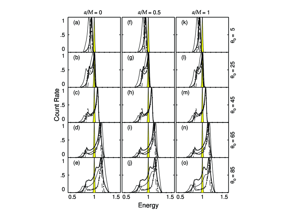
Figure 1: Synthetic emission-line profiles from a thin Keplerian disk with locally isotropic radiation and for three values of the black-hole dimensionless angular momentum: $a/M=0$ (left column), $a/M=0.5$ (center), and $a/M=1$ (right). Observer’s inclination $\theta_{\rm o}$ acquires values between $\theta_{\rm o}=0^{\rm{}o}$ (pole-on view) and $90^{\rm{}o}$ (edge-on). See the text for a detailed description and Tab. 2 for characteristics of the profiles.

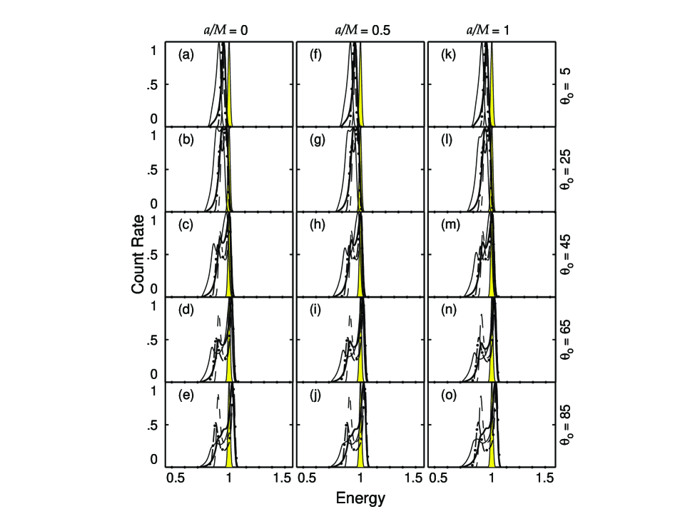
Figure 2: As in Fig. 1 but for a disk with radial component of the flow velocity comparable to the azimuthal component.

Figure 3: As in Fig. 1 but for locally anisotropic radiation.

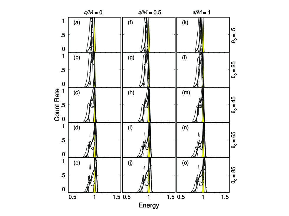
Figure 4: As in Fig. 2 but for locally anisotropic radiation.