The first section discusses a recalibration of the luminosity–linewidth technique and its use in a determination of ${\rm H}_{0}$. The recalibration introduces (i) new cluster calibration data, (ii) new corrections for reddening as a function of inclination, and (iii) a new zero-point calibration using 13 galaxies with distances determined via the cepheid period–luminosity method. It is found that H${}_{0}=82\pm 16$ km s^-1 Mpc^-1 (95% confidence).

The second section concerns a dynamic measurement of $\Omega_{0}$. The non-linear Least Action method can be used to reconstruct the orbits galaxies have followed to reach their current positions. The three free parameters of the models are M/L, age of the Universe, and a measure of the possible extended nature of dark halos compared with the distribution of light. Models are constrained by 900 observed distances. Best $\chi^{2}$ fits are for models with M/L values consistent with $\Omega_{0}=0.25\pm 0.2$.

The concept of ‘antibiasing’ is introduced in an attempt to reconcile this low estimate of $\Omega_{0}$ with the results from linear analyses. It is argued that M/L values in elliptical-rich regions are a factor of $7$ larger than those in spiral-rich regions. Hence, whereas it is commonly thought that there is the bias that mass is more extended than light, there may be a cosmologically important regime where there is the antibias of mass more concentrated than light. This possibility makes the inferrance of $\Omega_{o}$ from $\beta$ unclear.

1 The Hubble Constant

The Hubble Space Telescope (HST) has been used by three separate groups to detect cepheid variables in external galaxies, measure the luminosities of those stars, and determine distances to the host nebulae (Sandage et al. 1992; Freedman et al. 1994; Tanvir et al. 1995). The correlations between the global luminosities of galaxies and rotation velocities (Tully & Fisher 1977) are thought to produce good relative distances, but at the time of my previous calibrations of the zero-points in various wavebands (Pierce & Tully 1988, 1992) there were only five nearby galaxies with distance estimates based on observations of cepheids with ground-based telescopes. Now there are 13 suitable galaxies with cepheid distance determinations. The HST cepheid programs are about half completed. An interum recalibration of the zero-point at $B,R,I$ bands is provided in this paper.

Two other improvements are made. More optical, near-infrared, and radio HI data is available so the calibration samples are larger and more complete. Also, the spectral coverage provided by $B,R,I$,$K^{\prime}$ photometry leads to a better specification of the obscuration properties of galaxies.

1.1 The Cluster Samples

Malmquist bias caused by a magnitude limit (Malmquist 1920) can be neutralized if one has a suitable calibration sample. There are three requirements: one, the sample should be complete to an absolute magnitude limit fainter than the targets to be subsequently studied; two, the intrinsic properties of the calibrators should be statistically similar to the targets; three, the quality of the observations should be similar. With sufficient effort the completeness requirement can be met, and with sufficient care the quality of the observed material should be comparable between data sets. It is impossible to be certain that the intrinsic properties of the calibrators are truly representative but there can be some confidence in this proposition if several alternative calibration samples, representative of different environments, have consistent correlation slope and scatter characteristics.

The current calibration uses 89 galaxies in three rather different clusters. The obvious advantage of clusters is the possibility to achieve completeness within a volume to an absolute magnitude limit. The disadvantage is that cluster galaxies may be systematically different from those in the field. Two of the ‘clusters’ used in this study are poor specimens as clusters and were chosen because the environments are arguably the same as the ‘field’. The Ursa Major Cluster contains 62 galaxies with $M_{B}^{b,i}<-16.5^{m}$, no ellipticals, only 10 S0-S0/$a$ types, and the rest are spirals and irregulars with normal HI content. The cluster has no central core, the radial velocity dispersion is only $\sim 150$ km/s so a crossing time is $\sim 0.5{\rm H}_{0}^{-1}$, and it can be inferred that the region is in an early stage of collapse (Tully et al. 1996). Excluding galaxies with $i<45^{\circ}$, ${\rm T}<{\rm S}a$, and interacting/peculiar, leaves a sample of 37 objects. The Pisces ‘cluster’ has been used frequently for distance scale studies (Aaronson et al. 1986; Han & Mould 1992) but it, too, is composed mainly of HI-rich galaxies scattered about several insubstantial knots of early systems and may more properly be viewed as a prominent section of an intracluster filament (Sakai, Giovanelli, & Wegner 1994). Excluding galaxies with $i<60^{\circ}$, ${\rm T}<{\rm S}a$, interacting, or with insufficient $S/N$ in the HI signal leaves a sample of 25 objects with $M_{B}^{b,i}<-19^{m}$. The third sample comes from the Coma Cluster, certainly a very rich and dense environment quite unlike the field. A calibration based only on this cluster would be subject to justifiable criticism. However, it is found that the properties of the correlations are compatible between this extreme environment and the others which is an argument that the methodology works over a wide range of environmental conditions. The same exclusions as with Pisces leaves a sample of 27 objects with $M_{B}^{b,i}<-19.3^{m}$. In sum, 89 galaxies are used in the present analysis that satisfy magnitude completeness criteria. About 20 galaxies are missing from a truly complete sample to the present limits because the HI detections currently have insufficient $S/N$.

1.2 Revised Reddening Corrections

Photometry in four bands from $B$ to $K^{\prime}$, available for the UMa and Pisces samples, make it possible to refine the corrections that must be made for obscuration as a function of inclination. The most sensitive tests use deviations from mean color-magnitude correlations involving $K^{\prime}$. More inclined galaxies tend to be redder because of obscuration. Deviations from mean luminosity–linewidth correlations (more inclined galaxies tend to be fainter) can be used for independent but somewhat less sensitive tests.

Reddening may be different for different classes of galaxies. Giovanelli et al. (1995) have presented a strong case for a luminosity dependence among spiral systems. There is enough information now available to specify the gross characteristics of this dependency. The results from the 4-band color-magnitude analysis confirms the Giovanelli et al. claim. A simple linear dependence of the amplitude of reddening with magnitude is advocated at this time. The enhanced corrections toward the bright end of the luminosity–linewidth relations causes a steepening of the correlations, particularly at the shorter wavelength bands. As a consequence, there is a considerably weaker color dependence of the slopes than experienced previously. The new reddening corrections are discussed by Tully et al. (1998).

1.3 Zero-Point Calibration

The neutralization of Malmquist bias is achieved with regressions that accept errors in the distance independent variable (ie, the linewidths) in a sample that is complete to a limit in the distance dependent variable (ie, magnitudes). At a given magnitude, galaxies on either side of the mean linewidth are equally accessible. It is found that the slopes of the regressions on linewidth are compatible between the three cluster samples. Hence, it seems justified to slide the separate cluster correlations in magnitude to find the relative distance differences that result in a common correlation. A further constraint is provided by the requirement that the relative distances agree between the measurements at different passbands: the agreement between the $B,R,I$ filters is $0.03^{m}$ rms. We definite the slopes of the correlations and measure the relative distances of the three clusters. Pisces is determined to be $2.55^{m}$ farther away than UMa and Coma is determined to be $3.33^{m}$ farther away than UMa.

In the regime with $M_{B}^{b,i}<-16.5^{m}$, there are now 8 galaxies with HST cepheid measurements to add to 5 galaxies with ground-based distance determinations from cepheid observations. These 13 galaxies lead to luminosity–linewidth correlations that are consistent with the combined cluster slopes with even less scatter. There is no contradiction to the proposition that the calibrators are similar to the cluster galaxies in properties and provide a reasonable zero-point determination to the magnitude scale.

1.4 A Determination of H₀

The $R$ band luminosity–linewidth relation for the three clusters and calibrator data sets is displayed in Figure 1. Relations with similar scatter exist at $I$ and $K^{\prime}$ and, with greater scatter, at $B$. The calibrators have not been observed at $K^{\prime}$ so, as yet, only relative distances can be obtained at that band. The Ursa Major Cluster has a distance modulus of 31.33, or 18.5 Mpc. From the relative distances of the clusters, Pisces is at 60 Mpc and Coma is at 86 Mpc. Han & Mould (1992) report the mean redshifts of these clusters in the microwave background frame to be 4771 km s^-1 and 7186 km s^-1, respectively. The Pisces and Coma regions are sufficiently distant that their velocities may be a close approximation to the Hubble expansion. The distances to these clusters indicate H${}_{0}=80$ and $84$ km s^-1 Mpc^-1, respectively.

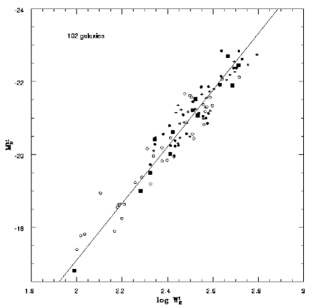
Figure 1.  : $R$-band luminosity–linewidth relation. The linewidth parameter $W_{R}^{i}$ is a transformation from the observed HI 20% linewidth to a value statistically equal to twice the maximum rotation velocity. Symbols denote the various samples: open circles–UMa, filled circles–Pisces, stars–Coma, filled boxes– calibrators with cepheid distances.

Statistical errors are estimated to be 8% from the typical rms scatter of $0.40^{m}$ and the numbers of objects in the samples. There is about a 7% uncertainty due to possible peculiar velocities of the two distant clusters. The present zero-point assumes a modulus of 18.50 for the Large Magellanic Cloud, uncertain to 10%. Systematic errors are estimated to be $<10\%$ from the observation that the scatter in the luminosity–linewidth relations is $\sim 0.4^{m}$ in case after case with consistency in slopes between different environments. Hence, systematics, apart from occasional blunders in photometry, are probably not a large fraction of the scatter; ie, $<1/2\times 0.4^{m}\sim 0.2$.

These results are $\sim 13\%$ higher than other recent recalibrations of luminosity–linewidth correlations (Mould et al. 1996; Giovanelli et al. 1997). Lower values of H₀ are coming from the distances found by the HST measurements of cepheids which tend to give host luminosities that are brighter at a given linewidth than found for the objects studied from the ground. Maybe it is just small numbers. There is about a 15% increase of the distance scale measured in this study from the new zero-point calibration.

On the other hand, there is a partially offsetting effect that comes about through the new absorption corrections. More luminous, highly inclined galaxies are made brighter. The galaxies in Pisces and Coma tend to be brighter than in UMa and the samples are restricted to more inclined systems in these clusters. Hence, overall they receive larger corrections and the cummulative effect is to give them smaller distances by roughly 8%.

Compared with earlier measurements, the new cepheid calibration has caused an increase in distances, but the revised reddening corrections has lead to smaller distances at larger redshifts. The overall mix produces a lower H₀ than before but only by $\sim 7\%$. It is sobering to see these systematics of order 10% and to appreciate that even these matters we know about are not well resolved. A current estimate of the Hubble parameter is H${}_{0}=82\pm 16$ km s^-1 Mpc^-1 (95% confidence) from the luminosity–linewidth method. This error does not include uncertainty in the zero-point attributable to the distance of the LMC. There is work yet to be done.

2 The Density Parameter

The measurements of galaxy distances can give a map of deviations from the Hubble expansion, something a few of us might find more interesting than the Hubble Constant issue. These deviant, or peculiar velocities are taken to arise from gravitational irregularities. Flows of galaxies are responding to perturbations on scales of tens of megaparsecs. Studies of these flows provide the opportunity to make a kinematic measurement of the distribution of dark matter on megaparsec scales and a determination of the cosmological density parameter $\Omega_{0}={\rm(mean~{}density)/(critical~{}density)}$.

2.1 The Method of Least Action

Shaya, Peebles, & Tully (1995) describe a non-linear method for the reconstruction of the orbits of a catalog of mass tracers. The orbits follow trajectories that extremize the ‘action’, the time integral of the Lagrangian. Boundary conditions on the orbits are the observed current sky positions and redshifts and the initial conditions that peculiar velocities were negligible. A choice of mass-to-light ($M/L$) ratio transforms the observed luminosities of the tracers into masses. These masses tug on each other over the age of the Universe. The Least Action model predicts a distance for each tracer. These model predictions are compared with observed distances in roughly 30% of cases. The match between model and observed distances provides a measure of the quality of the model.

At present, three parameters define a model. In the simplest case, there need only be two parameters. If mass is very closely coupled to the light then it is sufficient to identify only an $M/L$ ratio and an age of the Universe to specify the time that the masses pull on each other. A third parameter can be introduced to address the complexity of biasing. If matter is more widely spread than the light then close-passing halos might begin to merge. The effective masses will be reduced from the true masses. A gimic to recover the true masses is to introduce a ‘softening parameter’. Inside the scale of this parameter forces are reduced from the $r^{-2}$ expectation, so mass requirements are driven up.

2.2 Application to Simulations and the Real Universe

The Least Action procedure has been appplied to a standard Cold Dark Matter N-body simulation (Bond, Kofman, & Pogosyan 1996) to test if the method recovers the known $\Omega_{0}=1$ property of the model. If, naively, mass is assumed to be concentrated at the locations of the halo tracers then the Least Action reconstruction fails to recover all the mass. The known mass is recovered, however, if the softening parameter is taken to be $\sim 400$ km s^-1. Halos begin to inter-penetrate on roughly this scale.

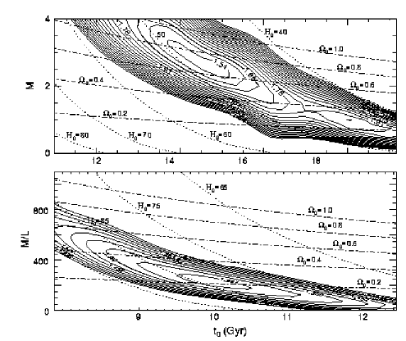
Figure 2.  : Top. $\chi^{2}$ map of Least Action models of a standard CDM N-body simulation. The vertical mass scale is in arbitrary units defined such that the true mass of the simulation is recovered with $M=4$. The heavy contour is at the $2\sigma$ level. Curves of $\Omega_{0}$ and H₀ are superposed. In this case, the force softening occurs on scales less than 250 km s^-1 which is too small to optimally recover the known parameters $M=4$, $\Omega_{0}=1$, H${}_{0}=50$. Bottom. Application to the real data. Force softening occurs on scales less than 300 km s^-1 in this case, slightly less than the case that produces the minimum $\chi^{2}$.

The same procedure has now been applied to the real Universe. A catalog of 3030 galaxies within 3000 km s^-1 describes the distribution of matter. Complex orbits are avoided by grouping galaxies in dense regions. A total of 1323 groups/galaxies are identified that should never have intersected with each other. The distribution of a combination of rich clusters and sources selected from complete redshift surveys drawn from the InfraRed Astronomy Satellite provide a description of tidal fields on scales greater than 3000 km s^-1. The consistancy of the model distances are tested by comparison with 900 measured distances. Most of these observed distances come from application of the luminosity–linewidth correlations discussed in the previous section but 50 distances come from either cepheids, or surface brightness fluctuations (Tonry, Ajhar, & Luppino 1990), or planetary nebula luminosity functions (Jacoby, Ciardullo, & Ford 1990).

In the simplest no-biasing case with mass distributed closely like the light then the Least Action procedure results in best fits with very low densities: $\Omega_{0}=0.14\pm 0.10$ (95% confidence). The error estimate is within the context of the no-bias assumption. Systematic uncertainties attributable to biasing are considerably larger. When the third parameter was admitted, $\chi^{2}$ fits improved with increasing values of the softening parameter until an optimum value of $\sim 400$ km s^-1 is reached. In this case, $\Omega_{0}=0.25\pm 0.2$. The uncertainty is larger, only approximate, and dominated by the vagaries of biasing. The $\chi^{2}$ fits for models near, but not quite, optimum are illustrated in Figure 2. Though a lot more intercomparisons between N-body simulations and the real data are required, it is reasonably convincing that the real world is not described by the standard CDM model.

2.3 Antibiasing

The concept of biasing in the distribution of galaxies (Kaiser 1984) arises from the reasonable possibility that starlight and dark matter may not always be strongly correlated in position. Dynamical interpretations of galaxy flows from linear analyses (Dekel, Bertschinger & Faber 1990; Hudson 1994; Davis, Nusser, & Willick 1996) measure the parameter $\beta$, with the relation to the physical parameter of interest $\Omega_{0}=(\beta b)^{1.7}$ where $b$ is the so-called ‘bias’ parameter: $b={\rm(observed~{}fluctuations)/(true~{}mass~{}fluctuations)}$. Experience with cosmological simulations and common sense give the appreciation that dark matter could be more widely distributed than the light of stars. The great voids in the distribution of galaxies may not be entirely empty of matter. In this scenario, the observed fluctuations in the galaxy distribution are a larger fraction of the mean than the fluctuations in the total mass. Hence, $b>1$ and $\Omega_{0}>\beta^{1.7}$.

At issue is why, by-and-large, the linear dynamical studies are claimed to give evidence for high values of $\Omega_{0}$, in the range $0.5-1$, (Dekel et al. 1990; da Costa et al. 1997; though $\beta$ values have been tending downward, see Riess et al. 1997) whereas the non-linear Least Action analysis persists in giving values well below closure. The non-linear analysis gives a direct measure of masses, hence of $\Omega_{0}$ with a suitable normalization, and the possibility of biasing in the measurement of masses is addressed within the modeling, for example, by the ’force softening’ trick. The premise with the linear analyses has been that the bias factor has the property $b\geq 1$. Here, the possibility is raised that $b<1$, that is, that mass fluctuations could be more concentrated than the light in some circumstances.

The evidence comes from the Least Action modeling of regions of collapse, particularly the infall region around the Virgo Cluster. There are galaxies falling on first approach toward the cluster with line-of-sight velocities with respect to the cluster of up to +900 and -600 km s^-1. These galaxies are not in the cluster; they are off the cluster in projection in the ‘southern extension’. Distance measurements show conclusively that they are within the infall region around Virgo rather than at the foreground or background ‘triple-value’ location outside the infall region. The envelope of peculiar velocities as a function of angular separation puts a strong constraint on the mass of the Virgo Cluster of $\sim 1.3\times 10^{15}M_{\odot}$ if the cluster is at a distance of 16 Mpc. This result implies $M/L\sim 1000M_{\odot}/L_{\odot}$. There is evidence of similarly high $M/L$ requirements in other elliptical-rich environments such as the Eridanus, Fornax, and Centaurus clusters.

There is the strong implication from the Least Action modeling that elliptical-rich environments have very large $M/L$ ratios. On the other hand, the $M/L$ values for the vast bulk of the mass tracers cannot be nearly so high. Indeed, if the elliptical-rich clusters are given the implicated high $M/L$ values then the residual mass requirements for the spiral-rich systems is modestly reduced. Best $\chi^{2}$ fits are coming in with $M/L\sim 150M_{\odot}/L_{\odot}$. Hence there is the extraordinary implication that $M/L({\rm E})\sim 7M/L({\rm S})$ where E means elliptical-rich environment and S means spiral-rich environment. This result was already found with the Virgo infall study by Tully & Shaya (1984). That earlier analysis used a non-linear but spherically symmetric model. It could have been feared that the approximation to symmetry gave an insecure result but the non-parametric Least Action model shows the earlier conclusion was sound.

Roughly 8% of the $B$ light within 3000 km s^-1 comes from elliptical-rich clusters. However, with a factor of 7 boost, some 40% of the mass could be in these knots! Roughly 10% of galaxies are in rich clusters, but maybe a much larger percentage of the collapsed matter is in these rich clusters. If so, then the bias factor is $<1$ at least in high density regions.

It is not hard to think of reasons why $M/L$ values might be considerably higher in dense clusters than in low density locations. Stellar populations are older and redder. Tidal stripping may have pulled stars out of galaxies in clusters and there is evidence that there might be a comparable number of stars in the intra-cluster space as in the galaxies. There are more baryons in hot intracluster gas than in stars in rich clusters. Gas in the primordial cloud around field galaxies will continue to rain down onto those galaxies perhaps even to the present epoch. By contrast, if a galaxy falls into a cluster then the gas from its primordial cloud cannot reach that galaxy because of the Roche limit set by the tidal field of the cluster (Shaya & Tully 1984). The gas supplies the intra-cluster medium not the galaxy.

It is plausible that the bias factor is a complicated function of environment, spatial scale, and passband. Mass may be more extended than light in low density regions and more concentrated than light in high density regions. Since the former effect has been called ‘biasing’, the latter effect can be called ‘antibiasing’. The claim made here is that the latter effect may be much more extreme than suspected, to the degree that it puts the sense of the correction $\beta\rightarrow\Omega_{0}$ in doubt.

3 References

Aaronson, M., Bothun, G., Mould, J.R, Huchra, J.P, Schommer, R.A., &

Cornell, M.E. 1986, Ap.J., 302, 536.

Bond, J.R., Kofman, L., & Pogosyan, D. 1996, Nature, 380, 603.

da Costa, L.N., Nusser, A., Freudling, W., Giovanelli, R., Haynes, M.P.,

Salzer, J.J., & Wegner, G. 1997, astro-ph/9707299.

Davis, M., Nusser, A., & Willick, J. 1996, Ap.J., 473, 22.

Dekel, A., Berschinger, E., & Faber, S.M. 1990, Ap.J., 364, 349.

Freedman, W.L. et al. 1994, Nature, 371, 757.

Hudson, M.J. 1994, M.N.R.A.S., 266, 468.

Giovanelli, R., Haynes, M.P., Salzer, J., Wegner, G., da Costa, L., & Freudling,

W. 1995, A.J., 110, 1059.

Giovanelli, R., Haynes, M.P., da Costa, L., Freudling, W., Salzer, J.J., &

Wegner, G. 1997, Ap.J., 477, L1.

Han, M.S. & Mould, J.R. 1992, Ap.J., 396, 453.

Jacoby, G.H, Ciardullo, R., & Ford, H.C. 1990, Ap.J., 356, 332.

Kaiser, N. 1984, Ap.J., 284, L9.

Malmquist, K.G. 1920, Medd. Lund Astron. Obs., Ser. 2, No. 22.

Mould, J., Sakai, S., Hughes, S., & Han, M. 1996, in The Extragalactic

Distance Scale, A.S.P. Series, ed. M. Livio.

Pierce, M.J., & Tully, R.B. 1988, Ap.J., 330, 579.

Pierce, M.J., & Tully, R.B. 1992, Ap.J., 387, 47.

Sakai, S., Giovanelli, R., & Wegner, G. 1994, Ap.J., 108, 33.

Sandage, A., Saha, A., Tammann, G.A., Panagia, N., & Macchetto, F.D.

1992, Ap.J., 401, L7.

Shaya, E.J., & Tully, R.B. 1984, Ap.J., 281, 56.

Shaya, E.J., Peebles, P.J.E., & Tully, R.B. 1995, Ap.J., 454, 15.

Tanvir, N.R., Shanks, T., Ferguson, H.C., & Robinson, D.T.R. 1995,

Nature, 377, 27.

Tonry, J.L., Ajhar, E.A., & Luppino, G.A. 1990, A.J., 100, 1416.

Tully, R.B., & Fisher, J.R. 1977, Astron. Astrophy., 54, 661.

Tully, R.B., Pierce, M.J., Huang, J.S., Saunders, W., Verheijen, M.A.W.,

Witchalls, P.L. 1998, to be submitted to A.J..

Tully, R.B., & Shaya, E.J. 1984, Ap.J., 281, 31.

Tully, R.B., Verheijen, M.A.W., Pierce, M.J., Huang, J.S., & Wainscoat,

R.J. 1996, A.J., 112, 2471.