Galaxy Formation and Evolution. I.
The Padua TREE-SPH code (PD-SPH)

Abstract

In this paper we report on PD-SPH the new tree-sph code developed in Padua. The main features of the code are described and the results of a new and independent series of 1-D and 3-D tests are shown. The paper is mainly dedicated to the presentation of the code and to the critical discussion of its performances. In particular great attention is devoted to the convergency analysis. The code is highly adaptive in space and time by means of individual smoothing lengths and individual time steps. At present it contains both dark and baryonic matter, this latter in form of gas and stars, cooling, thermal conduction, star formation, and feed-back from Type I and II supernovae, stellar winds, and ultraviolet flux from massive stars, and finally chemical enrichment. New cooling rates that depend on the metal abundance of the interstellar medium are employed, and the differences with respect to the standard ones are outlined. Finally, we show the simulation of the dynamical and chemical evolution of a disk-like galaxy with and without feed-back. The code is suitably designed to study in a global fashion the problem of formation and evolution of elliptical galaxies, and in particular to feed a spectro–photometric code from which the integrated spectra, magnitudes, and colors (together with their spatial gradients) can be derived.

The PD-SPH code

1 Introduction

The conventional picture of star formation in elliptical galaxies is one in which the galaxies and their stellar content formed early in the universe and have evolved quiescently ever since. This view is supported by the apparent uniformity of elliptical galaxies in photometric and chemical appearance (cf. Matteucci 1997 for a recent review) and the existence of scaling relations, e.g. the fundamental plane (cf. Bender 1997). In contrast, the close scrutiny of nearby elliptical galaxies makes evident a large variety of morphological and kinematic peculiarities and occurrence of star formation in a recent past (Schweizer et al. 1990, Schweizer & Seitzer 1992, Rampazzo et al. 1996). All this leads to a different picture in which elliptical galaxies are formed by mergers and/or accretion of smaller units over a time scale comparable to the Hubble time. Furthermore, strong evolution in the population of early type galaxies has been reported by Kauffmann et al. (1996) which has been considered to support the hierarchical galaxy formation model (Kauffmann et al. 1993, Baugh et al. 1996).

Tracing back the formation mechanism of elliptical galaxies from the bulk of their chemo-spectro-photometric properties is a cumbersome affair because studies of stellar populations in integrated light reveal only luminosity weighted ages and metallicities, and are ultimately unable to distinguish between episodic (perhaps recurrent) and monolithic histories of star formation and between star formation histories in isolation or interaction.

As nowadays most of the properties of elliptical galaxies have been studied with sophisticated chemo-spectro-photometric models in which the dynamical process of galaxy formation is reduced to assuming either the closed box or infall scheme and a suitable law of star formation (Arimoto & Yoshii 1987, 1989; Bruzual & Charlot 1993; Bressan et al. 1994; Worthey 1994; Einsel et al. 1995; Tantalo et al. 1996; Bressan et al. 1996; Gibson 1996a,b,c; Gibson 1997; Gibson & Matteucci 1996; Tantalo et al. 1997).

In contrast, the highly sophisticated dynamical models of galaxy formation (Hernquist & Katz 1989; Davis et al. 1992; Katz 1992; Steinmetz & Müller 1993; Navarro & White 1993; Nelson & Papaloizou 1994; Katz, Weinberg & Hernquist 1995; Navarro & Steinmetz 1997; Haehnelt et al. 1996a,b; Steinmetz & Mueller 1995; Navarro et al. 1996; Steinmetz 1996a,b and references), owing to the complexity of the problem are still somewhat unable to make detailed predictions about the chemo-spectro-photometric properties of the galaxies in question.

Attempts to bridge the two aspects of the same problem are by Theis et al. (1992 and references) and most recently by Contardo, Steinmetz & Fritze-v-Alvensleben (1997 in preparation).

This paper is the first of a series dedicated to the study of this complex problem in a self-consistent fashion, in which the formation and evolution of galaxies, together with their chemo-spectro-photometric properties, stem from a unique model able to predict a number of observable quantities to be compared with real data. The project aims to build dynamical models of disk-like and elliptical galaxies by means of the SPH (Smoothed Particle Hydrodynamics) technique, in which the effects of different initial conditions and basic physical processes, such as star formation, heating of the gas by various mechanisms (supernova explosions, stellar winds, UV fluxes), cooling of this by radiative atomic and molecular agents, interplay between dynamics and thermodynamics (feed-back), and chemical enrichment of the inter-stellar medium are taken into account. The models allow for the presence of dark matter and the effect of this on the gravitational field, which is described using Barnes & Hut (1986) treecode. The rates of star formation and chemical enrichment as function of space and time resulting from the dynamical models are meant to feed chemical-spectro-photometric models which should provide the kind of data (luminosities, integrated spectral energy distributions, broad band colors, line strength indices, etc.) to be compared with real observations for nearby and high redshift galaxies.

In this paper we present the first step toward this articulated analysis of the problem, i.e. the tool to construct dynamical models, and describe in some detail the numerical algorithm and the key physical ingredients. The dynamical models are based on the SPH technique, one of the most popular and efficient tool of modern studies of numerical hydrodynamics, and in astrophysical context of structures and galaxy formation. In the following we will refer to the SPH code we have developed as the Padua SPH (PD-SPH).

When SPH is coupled with an efficient scheme to compute gravity (like tree codes), it becomes a powerful tool to investigate physical situations of enormous complexity such as for instance, the formation and evolution of a galaxy (in the isolation picture) and/or the interaction-merge of galaxies (in the hierarchical scenario). The lagrangian nature of the method allows us to follow the evolution of physical quantities at all scales, provided that sufficient resolution is ensured.

The plan of the paper is as follows. Section 2 gives a detailed description of the code. Section 3 discusses tests in one dimension, i.e. the results for the Riemann problem and the convergency analysis, whereas section 4 contains tests performed in three dimensions. Section 5 presents the first astrophysical application, i.e. the collapse of a galaxy made of gas and dark matter in presence of initial solid body rotation. Section 6 thoroughly presents non–adiabatic processes, such as thermal conduction, radiative cooling, and heating by Type I and II supernova explosions, and stellar winds and ultraviolet radiation from massive stars that have used as source or sink of energy in our models. We adopt cooling rates that take the effect of metallicity into account. In Section 7 we describe the results obtained from our cooling prescription and compare them with those from metal independent cooling rates. Section 8 describes our prescriptions for the star formation rate and feed-back (rate of energy input from supernovae, stellar wind, and UV emission), and rate of chemical enrichment. Section 9 presents the results for two disk-like galaxies: the first case is with no feed-back of any type, whereas the second case is with feed-back. These models are not meant to represent real galaxies, first because the initial conditions are not derived from a cosmological context, second because the total number of particles is small owing to limitations in the computing facilities. The models are indeed meant to test the code response to various physical inputs. Nevertheless, despite the present limitations, the results are very promising. Finally, Section 10 presents some concluding remarks and outline the perspectives of future studies.

2 The PD-SPH code

PD-SPH is a TREE–SPH code, written in Fortran 90 (cf. Carraro 1995 & Lia 1996), conceptually similar to those described by Hernquist & Katz (1989) and Nelson & Papaloizou (1994). A 1-D version of the SPH code is in parallel form, and it has already been tested on the Cray T3D parallel computer hosted by CINECA (Benincà & Carraro 1995).

Schematically, PD-SPH uses $\rm SPH$ to solve the equations of motion for the gas component, and the Barnes & Hut (1986) octo-tree to compute the gravitational interactions. In this section we describe in some details the structure of the code and its basic ingredients.

It is widely known that SPH is a method standing on two basic ingredients: an interpolation using a kernel, and a Monte–Carlo evaluation of the physical quantities (Monaghan 1985). All relevant variables are interpolated in the following way:

$$\left\langle f({\vec{r}})\right\rangle=\int W({\vec{r}}-{\vec{r}}^{\prime},h)f({\vec{r}}^{\prime})\,d{\vec{r}}^{\prime},$$ (1)

where the integral is extended over the whole space and $W$ is a function generally referred to as the interpolating kernel; $h$ is the smoothing length determining the spatial region within which variables are smoothed, and governing the spatial resolution of the method.

The kernel is a spherically symmetric function strongly peaked at $\vec{r}=\vec{r}^{{}^{\prime}}$. It is easy to prove (Benz 1990) that these properties make SPH a second order technique, in which the estimate of any function is given by

$$\left\langle f({\vec{r}})\right\rangle=f({\vec{r}})+c(\nabla^{2}f)h^{2}+O(h^{3}).$$ (2)

This estimate is made in lagrangian formalism summing up the contributions of all the particles within $2\times h$, which represent the so–called neighbors.

2.1 Interpolating kernel

Three types of kernel can basically be found in literature: exponential, gaussian and spline; see Benz (1990) for more details. We have adopted the spline–kernel of Monaghan & Lattanzio, (1985):

$$W(r,h)=\frac{1}{\pi h^{3}}\left\{\begin{array}[]{ll}1-\frac{3}{2}u^{2}+\frac{3}{4}u^{3},&\mbox{se $0\leq u\leq 1$;}\\ \frac{1}{4}(2-u)^{3},&\mbox{se $1\leq u\leq 2$;}\\ 0.&\mbox{otherwise,}\end{array}\right.$$ (3)

and the supergaussian–kernel of Gingold & Monaghan, (1982):

$$W(r,h)=\frac{1}{\pi^{3/2}h^{3}}(\frac{5}{2}-u)exp(-u^{2}),$$ (4)

where $u=|{\vec{r}}|/h$.

The super–gaussian kernel is built up forcing the second order term in eq. (2) to be zero, It can be shown that this kernel corresponds to a fourth order interpolation. This kernel becomes negative for $r/h>\sqrt{5/2}$ (Benz 1990) and does not find an immediate physical interpretation.

Moreover, while the spline kernel is defined on a compact support, the super–gaussian kernel needs an artificial cut–off to limit the number of neighbors utilized in the estimate of the physical quantities. First, we checked both kernels (see Section 3 for details) and finally adopted the spline-kernel. In our code it is stored as a look–up table.

2.2 Evolution of the smoothing length and the search of neighbor particles

In SPH the spatial resolution is fixed by the smoothing length $h$. In our code $h$ is kept variable both in space and time according to Benz (1990)

$$\frac{dh}{dt}=-\frac{1}{3}\frac{h_{i}}{\rho_{i}}\frac{d\rho_{i}}{dt}=\frac{1}{3}h{\vec{\nabla}}{\vec{v}}.$$ (5)

This equation is added to the set of equations to be solved at any time–step. The main drawback of this approach is that in situations in which strong density gradients are present, it is not possible to keep under control the number of neighbors. Typically this number should be about 40–50 (Steinmetz & Müller 1993).

One possible solution is to artificially increase or decrease $h$ in order to keep fixed the neighbor number, but this involves several iterations if – as in our case – the tree-code is used to look for neighbors. As a consequence of this, the computational time gets often unacceptably long.

To cope with this difficulty, we have decided to maintain the above scheme when the neighbor number is lower than 40, and switch to the Nelson & Papaloizou (1994) formalism when the neighbor number is greater than 80. Accordingly the new smoothing length $h$ is

$$h_{i}=\frac{1}{N_{far}}\sum_{n=1}^{N_{far}}\frac{1}{2}|\vec{r}_{i}-\vec{r}_{n}|$$ (6)

where $N_{far}$ are the $n$ most distant nearest neighbors. We assume $N_{far}=10$.

There is another drawback in the Benz (1990) formalism that deserves some attention. The space–time variation of the smoothing length generally hampers the strict conservation of energy when terms involving the space derivatives of $h$ are not included. $\nabla h$ terms are essentially small correction (cf. the thorough discussion by Nelson & Papaloizou 1994), which do not significantly improve upon the conservation of energy.

Moreover the momentum conservation has been secured at an acceptable level of confidence also by symmetrizing the search of the nearest neighbors. In brief, a candidate particle $i$ is considered as a neighbor of $j$ if the following conditions are met

$$|{\vec{r}}_{i}-{\vec{r}}_{j}|<2\cdot h_{i}$$

or

$$|{\vec{r}}_{i}-{\vec{r}}_{j}|<2\cdot h_{j}.$$

Figure 1: Result of the shock tube problem using super-gaussian kernel (left panel) and spline kernel (right panel). In both cases 400 particles have been used. The arrow indicates the so–called blip in the pressure profile

2.3 Hydrodynamical equations

In PD-SPH, the particle forces and the specific energy are computed by means of the following equations

$$\frac{d\vec{v}_{i}}{dt}=-\sum_{j=1}^{N}m_{j}\left(\frac{\sqrt{P_{i}P_{j}}}{\rho_{i}\rho_{j}}+\Pi_{ij}\right)\times$$

$$\frac{1}{2}\left({\vec{\nabla}}_{i}W(r_{ij},h_{i})+\vec{\nabla}_{i}W(r_{ij},h_{j})\right))$$ (7)

and

$$\frac{du_{i}}{dt}=\sum_{j=1}^{N}m_{j}\left(\frac{\sqrt{P_{i}P_{j}}}{\rho_{i}\rho_{j}}+\frac{1}{2}\Pi_{ij}\right){\bf v}_{ij}\times$$

$$\frac{1}{2}\left({\vec{\nabla}}_{i}W(r_{ij},h_{i})+\vec{\nabla}_{i}W(r_{ij},h_{j})\right)+\Gamma_{R}-\frac{\Lambda_{C}}{\rho},$$ (8)

in which we adopt the arithmetic mean for the pressure gradient as in Hernquist & Katz (1989). Furthermore, in eq. (8) the first term represents the heating rate of mechanical nature (it is shortly indicated as $\Gamma_{M}$), the second term $\Gamma_{R}$ is the total heating rate from all sources apart from the mechanical ones, and the third term $\Lambda_{C}/\rho$ is the total cooling rate by many physical agents. These latter two will be discussed below in more detail. In the above equations $\vec{v}_{ij}=\vec{v}_{i}-\vec{v}_{j}$, and $\Pi_{ij}$ is the viscosity tensor defined as

$$\Pi_{ij}=\left\{\begin{array}[]{ll}\frac{-\alpha c_{ij}\mu_{ij}+\beta\mu_{ij}^{2}}{\rho_{ij}},&\mbox{if $(\vec{v}_{i}-\vec{v}_{j})\cdot(\vec{r}_{i}-\vec{r}_{j})>0$}\\ 0.&\mbox{otherwise,}\end{array}\right.$$ (9)

where

$$\mu_{ij}=\frac{h_{ij}({\vec{v}}_{i}-{\vec{v}}_{j})({\vec{r}}_{i}-{\vec{r}}_{j})}{|{\vec{r}}_{i}-{\vec{r}}_{j}|^{2}+\epsilon h_{ij}^{2}}.$$ (10)

Here $c_{ij}=0.5(c_{i}+c_{j})$ is the sound speed, $h_{ij}=0.5(h_{i}+h_{j})$, and $\alpha$ and $\beta$ are the viscosity parameters, usually set to 1.0 and 2.0, respectively. The factor $\epsilon$ is fixed to 0.01 and is meant to avoid divergencies.

As amply discussed by Navarro & Steinmetz (1997) this formulation has the disadvantage of not vanishing in the case of shear dominated flows, when $\vec{\nabla}\cdot\vec{v}=0$ and $\vec{\nabla}\times\vec{v}\neq 0$. In such a case, spurious shear viscosity can develop, mainly in simulations involving a small number of particles. To reduce the shear component we adopt the Balsara (1995) formulation of the viscosity tensor

$$\tilde{\Pi}=\Pi_{ij}\times\frac{f_{i}+f_{j}}{2},$$ (11)

where $f_{i}$ is a suitable function defined as

$$f_{i}=\frac{|<{\vec{\nabla}}\cdot{\vec{v}}>_{i}|}{|<{\vec{\nabla}}\cdot{\vec{v}}>_{i}|+|<{\vec{\nabla}}\times{\vec{v}}>_{i}|+\eta c_{i}/h_{i}},$$ (12)

and $\eta\approx 10^{-4}$ is a parameter meant to prevent numerical divergencies.

2.4 Time integration and stability criteria

Particle positions and velocities are updated, as in Hernquist & Katz (1989), using the leapfrog integrator and the multiple time–step scheme. The integration is of the second order in time, and proceeds as in the classical scheme.

Firstly an estimate of the velocity $\tilde{\vec{v}}_{i}^{n+1/2}$ is obtained from

$$\tilde{\vec{v}}_{i}^{n+1/2}={\vec{v}}_{i}^{n}+0.5\Delta t_{i}{\vec{a}}_{i}^{n-1/2}.$$ (13)

This is used to compute time-centered accelerations, ${\vec{a}}_{i}^{n+1/2}$, from which particle velocities and positions are updated

$${\vec{v}}_{i}^{n+1}={\vec{v}}_{i}^{n}+\Delta t_{i}{\vec{a}}_{i}^{n+1/2}$$ (14)

$${\vec{r}}_{i}^{n+1/2}={\vec{r}}_{i}^{n-1/2}+\Delta t_{i}{\vec{v}}_{i}^{n}.$$ (15)

The energy equation is explicitly solved, unless sink or source terms are present, and particle energies are advanced in the same manner as positions.

Time steps are calculated according to the Courant condition

$$\Delta t_{C,i}={\cal C}\frac{h_{i}}{h_{i}\left|\vec{\nabla}\cdot\vec{v}_{i}\right|+c_{i}+1.2(\alpha c_{i}+\beta max_{j}\left|\mu_{ij}\right|)},$$ (16)

with $\cal C$ $\approx 0.3$.

In presence of gravity, a more stringent condition on the time steps is required. According to Katz, Weinberg & Hernquist (1995), the additional criterion has to be satisfied

$$\Delta t_{G,i}=\eta\cdot MIN(\frac{\eta\epsilon}{|\vec{v}|},(\frac{\epsilon}{|\vec{a}|})^{1/2}),$$ (17)

where $\epsilon$ is the gravitational softening parameter and $\eta$ is another parameter usually set to 0.5. The final time step to be adopted is the smallest of the two

$$\Delta t_{i}=MIN(\Delta t_{C,i},\Delta t_{G,i}).$$ (18)

While the use of the multiple time step scheme may significantly speed up the code (Steinmetz 1995), sometimes the interpolations of non active particles may affect the energy conservation (see Section 4).

Figure 2: The number of particles involved in the blip versus the total number of particles in the simulation. $N_{blip}$ is on logarithmic scale

Figure 3: Blow-up of the contact discontinuity in the pressure profile. The left panel (a) shows the results obtained from adopting the super–gaussian kernel and the force term from Gingold & Monaghan (1983). The central (b) and right (c) panels show the same but for standard formalism for the pressure gradient and the super–gaussian and spline kernel, respectively. The dashed line is the analytical solution

Figure 4: Convergency test. The differences $\Delta$ between the numerical and analytical solutions for pressure and velocity profiles as a function of the total number of particle in the simulation

3 1-D numerical tests

The classical 1-D test to which SPH codes are compared is the Riemann shock tube problem. We use this test not only to check whether our code works properly, but also to analyse its convergency performances. The classical reference for this test is Gingold & Monaghan (1983), to whom we refer for the initial conditions of the problem. The time–steps and the smoothing lengths are constant, and fixed to 0.05 and 0.025, respectively. In other words, the smoothing lengths are set to be two times the maximum inter–particles separation. The particle masses (0.003125 in our case) are obviously chosen in such a way that the density and pressure profiles are matched (Gingold & Monaghan, 1983). The kernel is suitably normalized using the normalization constant $\frac{2}{3h}$ (see for instance Hernquist & Katz 1989.)

Figure 5: Convergency test. The differences $\Delta$ between the numerical and analytical solution in each of the four regions defined in the text. Open circles and crosses are for the minimum and maximum pressure. The continuous line represents the analytical solution

In Fig. 1 we show the results for pressure, density, velocity, and entropy of a simulation of the shock tube problem obtained using 400 particles and both the spline and super-gaussian kernel (right and left panels, respectively). The aim is to check whether using different kernels it might possible to eliminate the so called blip in the pressure profile (indicated by an arrow in Fig. 1). The nature of the blip is well known, and it is the signature of the contact discontinuity in the shock. In practice the pressure is discontinuous at this point, and the correspondent smoothed value $<Pr>$ is expected to be somewhat lower and higher at the left and right side of the contact discontinuity, respectively (Gingold & Monaghan 1983). Even if in our simulation the shock is broadened over a $4\times h$ region, the blip occurs as the signature of the unphysical step in the pressure.

We find that even using the super-gaussian kernel the blip albeit smoothed out does not disappear. In contrast to Gingold and Monaghan (1983), we are not able to eliminate the blip even using their new formulation for the pressure force

$$\frac{\nabla Pr}{\rho}=\rho^{\gamma-2}\left[\nabla(Pr\rho)+(\gamma-1)Pr\nabla\rho\right].$$ (19)

Instead of trying other expressions for the pressure gradient, once adopted a certain combination of kernel and pressure gradient, we prefer to run simulations with a different number of particles to check whether the SPH code can eventually recover the analytical solutions when larger and larger numbers of particles are used.

In Fig. 2 we show the number, $N_{blip}$, of particles involved in the blip as a function of the total number of particles $N_{tot}$ in the simulation. $N_{\it blip}$ is the number of particles counted in a searching sphere of radius equal to $2\times h$ near the blip location, and it is normalized to the total number $N_{tot}$. The results are as expected, in the sense that $N_{\it blip}$ strongly decreases at increasing $N_{tot}$, or equivalently at decreasing smoothing scale. These experiments show that the blip survives because of the still insufficient resolution.

In Fig. 3 we show the results of simulations performed using different combinations of kernels and gradient pressure terms. The region of interest is blown up for the sake of better understanding. Panel (a) is for super–gaussian kernel and the functional expression for $\frac{\nabla P}{\rho}$ by Gingold & Monaghan (1983). Panels (b) and (c) show the same but using the standard formalism for the pressure gradient, and adopting super–gaussian and spline kernel, respectively. In all the three panels the blip is clearly visible.

Figure 6: Adiabatic collapse: the evolution of the radial velocity profile (in units of $v_{\star}=(\frac{GM}{R^{2}})^{1/2}$) as a function of the age. The selected ages are the same as in Hernquist & Katz (1989)

Figure 7: Adiabatic collapse: the evolution of the specific internal energy profile (in units of $u_{\star}=\frac{GM}{R}$) as a function of the age. The selected ages are the same as in Hernquist & Katz (1989)

We notice, in particular, that the first combination of kernel and pressure gradient yields the best results, even if the numerical solution strongly departs from the analytical one. In the case with super–gaussian kernel and standard pressure gradient (panel b), the step in pressure is exactly the opposite of what is expected. Finally, in contrast with Gingold & Monaghan (1983), the inclusion of thermal conduction (cf. Lia 1996) does not eliminate the pressure step. Most likely, the blip is a feature intrinsic to the SPH smoothing itself.

As far as testing the convergency is concerned, we proceed as follows. We select four regions in the pressure profile, derive the maximum and minimum values from the numerical solutions at increasing number of particles in the simulation, and compare them with the analytical one. We choose the pressure as test physical quantity because of its sensitivity to the numerical technique. The pressure in fact is computed from the smoothed density and energy, instead of being directly smoothed out.

The four selected regions are the undisturbed warm fluid at the left of the shock (1), two regions near the shock, to the left (2) and to the right (3), respectively, and a region just to the right of the blip (4). These regions are centered at the linear coordinate $X$ = -0.6, -0.2, +0.04 and +0.2, respectively. The particles considered in the pressure evaluation are those contained in the $2\times h$ searching sphere.

The differences between numerical and analytical solutions are shown in Figs. 4 and 5.

In Fig. 4 we show the pressure (left) and velocity (right) differences $\Delta$ between numerical and analytical solutions at increasing number of particles in the simulation. The plotted differences are the mean of their values in the four test regions. As expected, the largest differences occur in the pressure profile. The four panels of Fig. 5 show the maximum and minimum values of the pressure in the four regions at increasing total number of particles as indicated. In each panel the horizontal line shows the analytical case by definition.

All these numerical tests prove the quick convergency of the numerical solution to the analytical one, and compared with the similar experiments by other authors, show that satisfactory agreement is achieved.

Finally, we like to report that the strong double–shocks tube experiment (cf. Steinmetz & Müller 1993) has also been successfully performed (Carraro 1995).

Figure 8: Adiabatic collapse. Upper panel: conservation of the potential (dashed-dotted line), kinetic (dotted line), thermal (dashed line), and total energy (continuous line). Lower panel: conservation of the total angular momentum

4 3-D numerical tests

In three dimensions we consider the adiabatic collapse of an initially non-rotating isothermal gas sphere. This is a standard test for SPH codes (Hernquist & Katz 1989; Steinmetz & Müller 1993; Nelson & Papaloizou 1994). To facilitate the comparison of our results with those by the above authors, we adopt the same initial model and the same units ($M=R=G=1$). The system consists of a $\gamma=5/3$ gas sphere, with an initially isothermal density profile:

$$\rho(r)=\frac{M(R)}{2\pi R^{2}}\frac{1}{r},$$ (20)

where M(R) is the total mass inside the sphere of radius R. Following Evrard (1988), the profile is obtained stretching an initially regular cubic grid by means of the radial transformation

$$r_{i}^{old}\Rightarrow r_{i}^{new}=(\frac{r_{i}^{old}}{R})^{3}R.$$ (21)

Alternatively it is possible to use the acceptance-rejection procedure by Hernquist & Katz (1989). The total number of particles used in this simulation is 2176. All the particles have the same mass. The initial specific internal energy is set to $u=0.05GM/R$.

4.1 Gravity

In PD-SPH, the newtonian forces are calculated using the Barnes–Hut tree-code (Barnes & Hut 1986). Tree-code is also used to perform the search of neighbors. We always include the multipole expansion, and smooth out the acceleration and the potential by means of the Hernquist & Katz (1989) formalism. We adopt the opening angle $\theta=0.8$, and tie the gravitational softening parameter $\epsilon$ to the particle number by looking at the mean inter-particle separation at half-mass radius. In the simulations below $\epsilon\approx 0.15$.

4.2 Description of the tests

The temporal evolution of the system is shown in the various panels of Figs. 6 and 7 which display the radial velocity and the specific internal energy, respectively. Each panel shows the variation of the physical quantity under consideration (in suitable units) as a function of the normalized radial coordinate at different time steps. These (in units of the dynamical time scale of the system) are exactly the same as in Hernquist & Katz (1989).

The initial low internal energy is not sufficient to support the gas cloud which starts to collapse. Approximately after one dynamical time scale a bounce occurs. The system can be described as an isothermal core plus an adiabatically expanding envelope pushed by the shock wave generated at the stage of maximum compression. After about three dynamical times the system reaches virial equilibrium with total energy equal to a half of the gravitational potential energy.

The temporal evolution of the potential and kinetic energies, and the total angular momentum is shown in Fig. 8. As pointed out by Nelson & Papaloizou (1994) the energy conservation, expressed as $\frac{\Delta E}{E}$ is $\approx 8\%$. This uncertainty is caused by neglecting $\nabla h$ terms and using multiple time steps. In brief, when the number of active particle gets too small, this causes fluctuations that may affect the energy conservation. Evolving the system with an unique time step for all the particle lowers the uncertainty on the energy conservation down to about $5-6\%$. As far as the angular momentum is concerned, this is conserved within one percent. Going back to the panels of Figs. 6 and 7 the present results agree fairly well with the mean values of the Hernquist & Katz (1989) models provided that the effects of the different number of particles are taken into account. For example the shock is located at the radial distance $0.18\leq r/R\leq 0.25$ in the models with age $t\approx 0.88$ (cf. the velocity panels of Fig. 6). The thermal energy slowly increases for $r/R\leq 0.1$ (cf. the panels of Fig. 7). Finally, at the time of maximum compression ($t\approx 1.1$), the dynamical range in the time steps is $20:1$. The scatter shown by the velocity and internal energy in the post shock phases is caused by the relative small number of particles, and the use of the multiple time step scheme. Similar scatter is present also in Steinmetz & Muller (1993) and Nelson & Papaloizou (1994).

Table 1: CPU time percentage in the adiabatic collapse.

Section of the code	Hernquist & Katz	This work
Gravitational computation	43.28	42.63
SPH computation	27.63	26.37
Search of the nearest neighbors	24.43	26.22
Tree construction	4.50	4.28
Miscellaneous	0.16	0.50

The above numerical tests have been performed on a Digital ALPHA OSF/1 workstation. It took about 5400 seconds of CPU time for 1019 time steps. It is worth comparing the CPU times required by different sections of our code with those by Hernquist & Katz (1989) . The comparison is summarized in Table 1. It appears that the fraction of CPU time spent in key sections of our code agrees with those of the Hernquist & Katz (1989) code.

5 Dark matter

We consider now a collapsing cloud of gas and dark matter with initial solid body rotation. The inclusion of dark matter is an important step, because it is known to play a key role in any modern theory of galaxy formation and evolution (cf. Frenk et al. 1996, Persic & Salucci 1997).

Initially, the dark matter particles have the same spatial distribution of the gas particles. Both in fact are obtained stretching an initial regular cubic grid (Evrard 1988). Therefore, dark matter and gas initially obey the same density profile.

Figure 9: Adiabatic collapse: the evolution of the dark matter component as a function of time in the X-Z plane. Time is in code units

Figure 10: Adiabatic collapse: the evolution of the baryonic component as a function time in the X-Z plane. Time is in code units

Figure 11: Collapse of a clump of gas and dark matter. Upper panel: conservation of the potential (dashed-dotted line), kinetic (dotted line), thermal (dashed line), and total energy (continuous line). Lower panel: conservation of the total angular momentum

This is a source of a technical difficulty with the tree-code algorithm because when two particles occupy the same position, the tree-code is not able to distinguish among them, when trying to divide the volume into elementary cells each of which containing either only one particle or no particles at all. This difficulty does not of course occur with the binary tree-code algorithm (cf. Benz et al. 1989). To handle this problem within a single tree-code scheme, we force the tree-code to consider a subdivision as an elementary cell also when two particles are enclosed provided that they are of different nature. This implies that every particle needs an additional flag specifying the species.

The system under consideration simulates a spherical galaxy whit total mass and radius of $10^{12}M_{\odot}$ and 100 kpc, respectively. In addition, the system is supposed to be made of equal numbers (2176) of particles in form of baryons and dark matter but with different individual mass such that the total mass fraction of baryons is 0.1 the total mass of the galaxy.

We adopt an initial solid body rotation around the Z–axis with angular velocity $\omega\approx 0.5$ which corresponds to a frequency of about 1 complete rotation in 10 free–fall time scales. So the effects of rotation get sizable during the collapse. This rotation corresponds to adopting the dimensionless spin parameter

$$\lambda=\frac{J|E|^{1/2}}{GM^{5/2}}=0.08$$

is somewhat larger than the value expected from the tidal torque in the hierarchically clustering universe theories, i.e. $\lambda\approx 0.05$ (White 1984, Steinmetz & Bartelmann 1996).

The gravitational softening parameters $\epsilon$ for gas and dark matter are in code units (see below) 0.002 and 0.010 to which 200 pc and 1 kpc correspond, respectively. They have been fixed on the basis of the Evrard (1988) relation

$$\frac{Gm}{\epsilon}\ll\frac{GM}{R}.$$ (22)

The parameter $\epsilon$ is kept constant in time for each individual particle. However if in a cell two particles of different nature (gas and DM) co–exist, the softening parameter is the mass weighted mean value.

Tests similar to those described below can be found in Navarro & White (1993) to which our results can be compared. In this context, the most salient result of the Navarro & White (1993) calculations is the different evolutionary behaviour of the dark matter and baryonic components. The same results are recovered here as shown in Figs. 9 and 10, respectively. In our models, however, the difference is less pronounced because of the lower initial spin as compared to $\lambda=0.10$ in Navarro & White (1993). In brief, dark matter gets a more flattened spatial distribution than the baryonic component. In fact equidensity contours of the baryons must coincide with equipotentials which are much rounder than contours of equal total density. It is worth recalling that observational hints for flatter dark halos have been found in galaxies like NGC 5907 (Sackett et al. 1994), NGC 4244 (Olling 1996), and NGC 891 (Becquaert & Combes 1997).

6 Non adiabatic processes

As far as the evolution of the gaseous component is concerned, all non adiabatic processes but artificial viscosity are of paramount importance. They drive in fact the energy and momentum loss or gain of these ”particles”. Since the final target is to follow the evolution of a real galaxy, processes like cooling and heating, star formation, and feed-back play a dominant role, and must be included from the very beginning in order to obtain results worth to be compared with observational data. Unfortunately, some of these processes are not yet well understood. The physics of star formation, in particular, is far from being assessed so that parameterizations of this basic process are imposed.

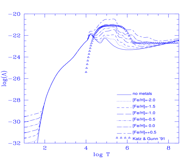
Figure 12: Net cooling rate $\Lambda_{C}/n^{2}$ in ergs $\rm cm^{-3}~{}s^{-1}$ as a function of temperature. $n$ is the number density of particles. The cooling rate is from Sutherland & Dopita (1993) for $T\geq 10^{4}$, Hollenbach & McKee (1979) and Tegmark et al. (1996) for $100\leq T\leq 10^{4}$, and Caimmi & Secco (1986) and Theis et al. (1992) for $T\leq 100$ K. Each curve corresponds to a different metallicity as indicated. For comparison the cooling rate by Katz & Gunn (1991) is superposed (open triangles)

In this section we present in some detail our assumptions concerning thermal conduction and cooling processes of the gaseous component, which are known to regulate the energy budget of a fluid element. They are included in the energy equation as source terms.

6.1 Thermal conduction

Thermal conduction is calculated according to the formalism developed by Monaghan & Lattanzio (1991)

$$\frac{1}{\rho}\vec{\nabla}\cdot(\rho q\vec{\nabla}u).$$ (23)

The translation of it into the SPH language is

$$\sum_{j=1}^{N}m_{j}\frac{(q_{i}-q_{j})(u_{i}-u_{j})\vec{r}_{ij}\cdot\vec{\nabla}W(\vec{r}_{ij},h)}{\rho_{ij}(r_{ij}^{2}+\eta^{2})},$$ (24)

where $q$ is the thermal conductivity function. This is in turn evaluated as

$$q_{i}+q_{j}=gh(c_{ij}-4\cdot\mu_{ij}),$$ (25)

In the above relations, $\eta$ is a parameter securing that the denominator of relation (25) remains different from zero, and and $g$ is another suitable parameter set equal to 0.25.

Thermal conduction is expected to be effective in situations of strong shocks, and/or ”wall heating” when two flows or two fluid elements collide. Thermal conduction is a source of heating in the energy equation (see below).

6.2 Cooling

Radiative cooling is the crucial mechanism responsible for condensation and collapse of baryonic gas into galaxies and, inside galaxies, for the occurrence of star formation. Cooling processes are rather well known, and have already been included in current models of galaxy formation and evolution albeit in different detail. See for instance Katz, Weinberg & Hernquist (1995) for a very accurate treatment of cooling processes of different nature. Among the various cooling agents we recall: (i) the radiative cooling by atomic and molecular processes; (ii) the inverse Compton mechanism in presence of microwave background radiation.

Radiative cooling. The most commonly used radiative cooling functions are those by Katz & Gunn (1991) because they are analytical and continuous with their first derivatives. These radiative cooling functions are calculated assuming the typical helium abundance by mass Y=0.25. They do not contain, however, the dependence on metallicity which in contrast is expected to be important during the evolution of a galaxy, as a natural consequence of the chemical enrichment. To cope with this drawback of the Katz & Gunn (1991) cooling functions, we adopt here those elaborated by Chiosi et al. (1997). In brief, these cooling function $\Lambda_{C}(u_{i},\rho_{i},Z_{i})$ are derived from literature data, and include different radiative processes. For temperatures greater than $10^{4}$ K they lean on the Sutherland & Dopita (1993) tabulations for a plasma under equilibrium conditions and metal abundances [Fe/H]=-10 (no metals), -3, -2, -1.5, -1, -0.5, 0 (solar), and 0.5. For temperatures in the range $100\leq T\leq 10^{4}$ the dominant source of cooling is the $H_{2}$ molecule getting rotationally or vibrationally excited through a collision with an $H$ atom or another $H_{2}$ molecule and decaying through radiative emission. The data in use have been derived from the analytical expressions of Hollenbach & McKee (1979) and Tegmark et al. (1996). Finally, for temperatures lower than 100 K, starting from the relation of Theis et al. (1992) and Caimmi & Secco (1986), they corporate the results of Hollenbach & McKee (1979), and Hollenbach (1988) for CO as the dominant coolant. The following analytical relation in which the mean fractionary abundance of CO is given as a function of [Fe/H], is found to fairly represent the normalized cooling rate (i.e. $\Lambda_{C}(CO)/n^{2}$ with $n$ the number density of particles)

$${\Lambda_{C}(CO)}=1.6\times 10^{-29}10^{([Fe/H]-1.699)}T^{0.5}~{}~{}\rm erg~{}cm^{3}~{}s^{-1}.$$ (26)

The normalized cooling rate (in units of $erg~{}cm^{3}~{}s^{-1}$) over the whole temperature range is shown in Fig. 12, in which the effects of the metallicity are clearly visible. It is worth mentioning that no re-scaling of the cooling rate from the various sources has been applied to get the smooth curves shown in Fig. 12. For the purposes of comparison, we display in Fig. 11 the cooling rate of Katz & Gunn (1991). The major point of disagreement is soon evident because their cooling rate which by definition is for a zero-metal composition actually lies well above the zero-metal curve of Sutherland & Dopita (1993). This implies that Katz’ & Gunn’s (1991) cooling is unphysically more efficient in situations of nearly zero metallicity, such as the protogalactic phase.

Figure 13: Testing cooling: the final distribution in $X-Z$ plane for gas particles in simulations with different cooling prescriptions. The right panel is for the cooling rate by Katz & Gunn (1991), whereas the left panel is for the cooling prescription described in the text

Figure 14: Cooling radiation (in code units): the solid line is with the cooling rate by Katz & Gunn (1991), whereas the dashed line is for the cooling rate used in this paper

Figure 15: Conservation of energy and angular momentum in a collapsing galaxy with the cooling rate adopted in this paper. The model is the same as in the left panel of Fig.13

Inverse Compton. We do not take into account inverse Compton cooling because of its strong dependence on redshift (Ikeuchi & Ostriker 1986). During the protogalactic phase of the evolution of a galaxy, from which we start our simulations, the inverse Compton cooling has already got much lower than the radiative cooling, so that it can be neglected.

Although the cooling rate has been derived over a wide range of temperatures from a few degree to above $10^{8}$, in reality only the portion above a suitable temperature $T_{min}$ can be used in model calculations because of the maximum resolution achievable in the N-body simulations. This limit is derived from imposing that the Jeans mass does not fall below a critical value, which is conventionally assumed to be the mass of four gas particles (cf. Katz & Gunn 1991). The limit temperature is given by the Bonnor-Ebert expression (Ebert 1955, Bonnor 1956)

$$T_{min}=0.89553\left[\left(\frac{4m_{p}}{\rho_{g}}\right)^{2/3}-\left(\frac{\pi\epsilon_{g}^{3}}{3}\right)^{2/3}\right]\frac{\mu m_{H}G}{k}\rho_{g},$$ (27)

where $m_{p}$ is the mass of a baryonic particle, $k$ is the Boltzmann constant, $\mu$ and $\epsilon$ are the mean molecular weight and the gas gravitational softening parameter, respectively.

The limit temperature $T_{min}$ is locally computed for every gas particle. Finally, the cooling functions are stored in the code as look-up tables.

6.3 Heating

Heating of the gas is caused by many processes among which we consider the thermalisation of the energy deposit by supernova explosions (both Type I and II), stellar winds from massive stars, the ultraviolet flux from massive stars, the cosmic ultraviolet flux, and finally sources of mechanical nature.

Supernovae. The rate of supernova explosions $R_{SNI,II}(t)$ over the time interval $\Delta t$ is calculated according to standard prescriptions (cf. Bressan et al. 1994; Tantalo et al. 1996, 1997; Greggio & Renzini 1983 for Type I SN in particular). Knowing the amount of energy released by each SN explosion, the total energy injection over the time interval $\Delta t$ is the sum of two terms, $E_{SNI}$ and $E_{SNII}$, of type

$$E_{SNI,II}=\int_{\Delta t}\epsilon_{SNI,II}R_{SNI,II}(t^{\prime})dt^{\prime},$$ (28)

where $R_{SNI,II}(t)$ is the number of supernovae per unit time, and $\epsilon_{SNI,II}$ is the energy injected per SN explosion. This formulation slightly differ from the one commonly adopted in chemical models of galaxies, in which $\epsilon_{SNI,II}$(t) is the thermalisation law of SN remnants include of the cooling processes (cf. Bressan et al. 1994, Tantalo et al. 1996, and Gibson 1995). In our scheme, first cooling effects are left to the energy budget equation, second owing the limitations implicit in the N-body technique we are not yet able to resolve the star forming fluid to the level of individual stars but only to that of massive cluster-like structures in which star can be formed according to a given initial mass function (see below). Therefore, following in detail the thermalisation law of SN is impossible. A reasonable compromise is obtained by using sufficiently small time steps (cf. also Chiosi et al. 1997 for a similar approach). The explicit formulations for $R_{SNI,II}(t)$ will be presented in the next section.

Stellar winds. The rate of energy injection by stellar winds is

$$E_{W}=\int_{\Delta t}\epsilon_{W}R_{W}(t^{\prime})dt^{\prime},$$ (29)

where $R_{W}$ is the number of stars per unit time expelling their envelopes during the time interval $\Delta t$ and, in analogy with the SN remnants, $\epsilon_{W}$ is the kinetic energy of stellar winds. A losing mass star is expected to deposit into the interstellar medium the energy

$$\epsilon_{W0}=\eta\times{M_{ej}(M)\over 2}({Z\over Z_{\odot}})^{0.75}\times v(M)^{2},$$ (30)

where $M_{ej}(M)$ is the amount of mass ejected by each star of mass $M$, $v(M)$ is the velocity of the ejected material, and $\eta$ is an efficiency factor of the order of 0.3 (Gibson 1994 and references therein). The calculation of the rate $R_{W}(t)$ is postponed to the next section.

Ultraviolet flux from massive stars. The rate of energy injection from the ultraviolet flux emitted by massive stars is

$$E_{UV}=\int_{\Delta t}\epsilon_{UV}R_{UV}(t^{\prime})dt^{\prime},$$ (31)

where $R_{UV}$ is the number of massive stars per unit time whose mass is the range $10~{}\div~{}120~{}M_{\odot}$, and $\epsilon_{UV}$ is the amount of ultraviolet energy emitted by each star. To calculate $\epsilon_{UV}$ the following procedure is adopted. We suppose that massive stars are located on the zero age main sequence, i.e. obeying well known mass-luminosity-effective temperature relationships, $L/L_{\odot}(M/M_{\odot}$) and $T_{eff}(M/M_{\odot}$). In principle, there should be an additional dependence on the chemical composition which, however, can be neglected here. The relationships $L/L_{\odot}(M/M_{\odot}$) and $T_{eff}(M/M_{\odot}$) are taken from the library of stellar models/isochrones of Bertelli et al. (1994 and references therein). For the sake of simplicity we can approximate the spectral energy distribution of any such stars as pure black body emission of given $T_{eff}$, for which we can immediately estimate the fraction $F_{UV}(M)$ of flux emitted short-ward of 4000 Å (our range for UV light) by a star of mass M. The UV flux emitted by each star is

$$\epsilon_{UV}=F_{UV}(M)\times L(M),$$ (32)

where $L$ is the total luminosity of the star. Once again the calculation of $R_{UV}(t)$ is postponed to the next section.

Cosmic UV radiation. As far as $UV$ radiation field is concerned, its effects have been thoroughly investigated by Navarro & Steinmetz (1996) who reached the conclusion that the cosmic $UV$ radiation plays some role only when the gas has already accreted onto the protogalaxy from the surrounding medium. Heating by cosmic UV radiation is not included in the present models. In this context, it is worth recalling that all models in which the cosmic UV radiation is the sole source of heating face the so-called overcooling problem (cf. Navarro & Steinmetz 1996).

Total radiative heating. The total heating rate due to radiative processes $H_{R}(u_{i},\rho_{i},Z_{i})$ to be included in the energy budget equation (see below) is

$$H_{R}={E_{SNI}+E_{SNII}+E_{W}+E_{UV}\over\Delta t}$$ (33)

Mechanical heating. In principle there are various mechanical processes that contribute to heat gas particles. Two of them have been explicitly taken into account in the basic energy equation (8). They have been shortly referred to as $\Gamma_{i,M}$ and are general functions of type $\Gamma_{i,M}(u_{i},\rho_{i},Z_{i})$.

6.4 More details on the energy equation

At this stage of the analysis we can write down the detailed expression of the energy equation in all its components. To this aim we need only to convert the radiative heating into the conventional SPH formalism

$$\Gamma_{R,i}(u_{i},\rho_{i},Z_{i})=\sum_{j}H_{R,j}\times{m_{j}\over\rho_{j}}W(i,j)$$ (34)

with obvious meaning of the symbols. The final energy equations is

$${du_{i}\over dt}=\Gamma_{M,i}+\Gamma_{R,i}(u_{i},\rho_{i},Z_{i})-{\Lambda_{C,i}(u_{i},\rho_{i},Z_{i})\over\rho_{i}}$$ (35)

with

$$\Gamma_{R,i}(u_{i},\rho_{i},Z_{i})=H_{C,i}(u_{i},\rho_{i},Z_{i})+H_{R,i}(u_{i},\rho_{i},Z_{i})$$ (36)

where $\Gamma_{R,i}$ the sum of thermal conductivity and all radiative heating sources. The energy $u_{i}$ is per unit mass, whereas all other quantities are per unit mass and time.

The functional dependence of the cooling term imposes an implicit solution of the energy equation. This is performed using an hybrid scheme, i.e. a combination of the Newton-Raphson and bisection methods. The associated second order updating of the thermal energy follows the technique of Hernquist & Katz (1989).

Finally, it is worth mentioning that under high cooling efficiency situations can be met in which the energy may become negative. To cope with this unphysical result of mere numerical nature we impose that a gas particle cannot lose more than a half of its thermal energy per time step (Hernquist & Katz 1989).

7 Testing cooling prescriptions

In this section we show an ideal galactic model in which no star formation, no chemical enrichment, and no energy deposit from the various sources are let occur. This model is meant to show the net results of different prescriptions for the cooling rate. The model has zero-metal content and apart from the cooling rate, it is identical to that by Katz & Gunn (1991) so that the comparison is possible.

We simulate the collapse of a spherical galaxy with mass of $10^{12}M_{\odot}$ and radius of 100 kpc. Like in the previous test the baryon fraction is 0.1, while the initial gas temperature is $10^{4}~{}^{o}\rm K$. In this simulation, time, spatial coordinates, energy, and density are expressed in the following units: $\rm[time]=7.41\times 10^{8}year$, $\rm[space]=100~{}\rm kpc$, $\rm[energy]=4.30\times 10^{14}erg~{}gr^{-1}$, and $\rm[density]=1.61\times 10^{-25}gr~{}cm^{-3}$. The temporal evolution of the models has been followed up to the age of 2.2 dynamical times ($\ approx1.6Gyr$).

The results are schematically presented in Figs. 13 and 14. Fig. 13 shows the distribution of particles on the $X-Z$ plane at three different ages (in code units) for our cooling rate, left panels, and Katz & Gunn (1991), right panels, whereas Fig. 14 compares the cooling radiation for the two assumptions for the cooling rate.

As the zero-metal cooling rate of Sutherland & Dopita (1993), on which our prescription stands for temperatures above $10^{4}$ K, is much less efficient than that of Katz & Gunn (1991), this easily explains why significantly longer time scales are need to form disk structures (cf. Fig. 13), and the much lower amount of radiated energy (cf. Fig. 14).

Finally, in Fig. 15 we show the conservation of total energy and angular momentum as a function of time for the case with the new cooling rate. The small decrease of the total energy at increasing time is caused by the lost of thermal energy radiated away by cooling processes (for comparison see the detailed trend of energies in Fig. 11). Angular momentum is conserved within 5% accuracy (see also Fig. 11 for comparison).

8 Going toward complete models: star formation, feed-back, and chemical enrichment

Implementing star formation into N-body simulations of galaxies is a cumbersome affair, reflecting partly our poor knowledge of this fundamental process, and partly the limitations still imposed by N-body technique itself.

To accomplish the task two basic steps are required: firstly we need to determine the star formation rate (SFR), and secondly we must treat the effects of the star formation on the interstellar medium (the so-called feed-back).

Figure 16: Simulation of a disk-like galaxy with no feed-back: the spatial distribution of gas (left panel) dark matter (central panel) and stars (right panel). Starting from the bottom the three panels of each raw refer to ages of 0.5, 2.5, and 5 Gyr

8.1 Star formation rate

To include star formation in the N-body scheme two important informations are needed: firstly we have to set suitable conditions under which stars can form, secondly we must express the SFR law governing the efficiency at which gas is turned into stars (cf. Steinmetz 1995 for a review on the subject).

When to form stars? There are at least three physical conditions to be met in order to activate the star forming process. First, a fluid element is eligible to make stars if it is part of a convergent flow, i.e. the particle velocity divergence must verify the condition

$$\vec{\nabla}\cdot\vec{v}_{i}<0.$$ (37)

Second, the fluid element must be Jeans unstable

$$\frac{h_{i}}{c_{i}}>\frac{1}{\sqrt{4\pi G\rho_{i}}}.$$ (38)

Finally, the gas particle must remain cool

$$\tau_{cool}\leq\tau_{ff}.$$ (39)

This last condition is usually translated into an overdensity criterion. For instance, Navarro & White (1993) uses the following expression

$$\rho_{i}>\rho_{crit},$$ (40)

where $\rho_{crit}=7\times 10^{-26}g~{}~{}cm^{-3}$. This minimum threshold density actually holds only in the case of a single cooling function (no dependence on chemical composition). However, as star formation causes metal enrichment of the interstellar medium, the threshold moves towards lower values at increasing metallicity. Because of this, we prefer to adopt condition (39) which is of general validity.

Figure 17: Simulation of a disk-like galaxy with no feed-back: the same as in Fig. 16 but onto the X-Y plane

Star formation law. A very popular, empirically based, rate of star formation is the Schmidt (1959) law, according to which

$$\Psi(t)=\frac{d\rho_{gas}}{dt}=-\frac{d\rho_{star}}{dt}=c_{\star}\frac{\rho_{gas}}{\tau_{ff}},$$ (41)

where $c_{\star}$ is the specific efficiency (in most cases a free parameter).

In dense regions (the ones prone to star formation), the cooling time $\tau_{cool}$ is typically much shorter than the dynamical time $\tau_{ff}$. Since $\tau_{ff}\propto\rho_{gas}^{-1/2}$, the SFR is proportional to $\rho_{gas}^{3/2}$, a result that agrees with Schmidt’s (1959) observational estimates. In most numerical simulations, the specific efficiency is taken to be $c_{*}=0.1$.

8.2 Star-like particles

When star formation has started, at any time-step $\Delta t$ a star-like particle is created, whose mass is

$$m_{\star}=m_{gas}\times(1-exp(-\frac{c_{\star}\Delta t}{\tau_{ff}})).$$ (42)

and the mass of the parent gas particle is consequently reduced. The above relation simply follows from integrating equation (41) over the time step $\Delta t$. The mass of the star-like particles obviously depends on the resolution (number of particles) of the simulation.

The star-like particle is supposed not to immediately acquire its own individuality, but to leave the parent gas particle only when the mass of this latter falls below a certain value (typically $50\%$ of the original mass). Furthermore, recurrent episodes of star formation within the same gas particle are possible, so that gas is depleted in discrete steps. Finally, the star-like particle it treated as a collisionless object. Therefore, the element of fluid in which star formation occurs is considered as a hybrid particle, whose collisional component experiences both hydrodynamical and gravitational forces, while its collisionless component feels only the gravitational field.

To avoid non physical accelerations due to the sudden decrease of the gas mass, particles in which star formation is active are stored in the lowest time-bin.

When a star-like particle leaves its parent, it inherits its position in the phase space, and its gravitational softening parameter. Resolution limitations force on us to consider only four star formation events per gas particle, like in Navarro & White (1993).

Figure 18: Simulation of a disk-like galaxy with no feed-back: the rates of star formation (top panel) and supernova explosions (Type II middle panel, Type I bottom panel)

Figure 19: Simulation of a disk-like galaxy with no feed-back: the age-metallicity relation for the gas component in the galactic disk. Filled circles show the age-metallicity relation of Disk stars in the Solar Vicinity by Edvardsson et al. (1993)

8.3 Feed-back

To quantitatively evaluate the feed-back by all heating processes already outlined in the previous section, we need to know the initial mass function, according to which the newly borne stars will distribute by number in each mass interval $dM$. For the sake of simplicity we adopt here the classical Salpeter (1955) law

$$\Phi(M)dM=A\cdot M^{-x}dM,$$ (43)

where $x=2.35$ (the Salpeter value) and $A$ is the normalization constant. This is derived from imposing that stars can be formed with masses in the range $0.1\div 120M_{\odot}$, and assuming that the integral of eq. (43) over this mass range is equal to one. It is worth recalling that only stars more massive than about 0.9 $M_{\odot}$ will be able to pollute the interstellar medium over a time scale shorter than the Hubble time (cf. Tinsley 1980, Matteucci 1997). The normalization constant is $A=0.06$. Other IMFs are already implemented into the code (Miller & Scalo 1979).

Supernova rates In the standard scenario of stellar evolution (cf. Woosley 1986, Chiosi 1986; Greggio and & Renzini 1983) Type II supernovae occur in single stars more massive than say 8 $M_{\odot}$, whereas Type I (more precisely Ia) supernovae occur in binary stars containing a re-juvenated white dwarf brought to explosion via the C-deflagration mechanism by mass accretion from the companion. Furthermore, Type II supernovae from progenitors more massive than say 30 $M_{\odot}$ leave behind a black hole (scarcely contributing to the enrichment of the interstellar medium in heavy elements), whereas Type II supernovae from progenitors in mass range 8 to 30 $M_{\odot}$ leave a neutron star and most effectively contribute to chemical enrichment in heavy elements. Type I supernovae have binary system progenitors with typical total mass in the range 3 to 16 $M_{\odot}$.

Figure 20: Simulation of a disk-like galaxy with full feed-back: the spatial distribution of gas (left panel) dark matter (central panel) and stars (right panel). Starting from the bottom, the three panels of each raw refer to ages of 0.5, 2.5, and 5 Gyr

To evaluate the rate of Type I occurrence one has to know the percentage of binary systems with respect to single stars. Let C be this fraction. Following Greggio & Renzini (1983), the rate of Type I supernovae is

$$R_{SNI}=C\int_{M_{B,inf}}^{M_{B,max}}\Phi_{B}(M_{B})dM_{B}\times$$

$$\int_{\mu_{inf}}^{1/2}2^{\gamma+1}(1+\gamma)\mu^{\gamma}\Psi[t-t_{(\mu M_{B})}]d\mu.$$ (44)

In the above expression $M_{B}$ is the total mass of the binary system, $\Phi_{B}(M_{B})$ is the IMF of binary stars, which is assumed here to be the same as for single stars [eq.(43)] for the sake of simplicity, $\mu=\frac{M_{2}}{M_{B}}$ is the fractionary mass of the secondary, which drives the evolution, and $\gamma$ is a coefficient, usually equal to 2. Finally, $M_{B,inf}$ and $M_{B,max}$ are the lower and upper limits for the total mass of the binary stars, respectively, and $\mu_{inf}$ is the lower limit for the fractionary mass of the secondary. These masses are calculated with the following receipt

$$M_{B,inf}=MAX(2M_{2},2),$$ (45)

$$M_{B,max}=8+M_{2},$$ (46)

$$\mu_{inf}=MAX(M_{2}(t)/M_{B},1/2).$$ (47)

Finally, $\Psi(t)$ is the SFR at the time equal to the difference between the current time and the lifetime of $M_{2}$.

The total rate of Type II supernovae is

$$R_{SNII}=\int_{M_{B,max}}^{120}\Phi(M)\\ Psi(t_{M})dM+$$

$$~{}~{}~{}~{}~{}~{}~{}~{}~{}~{}~{}~{}~{}~{}~{}~{}~{}(1-C)\int_{8}^{M_{B,max}}\Phi(M)\Psi(t_{M})dM$$ (48)

with obvious meaning of the symbols. Finally, the constant $C$ above is calibrated looking at the rate of Type Ia supernovae in spiral galaxies (van den Bergh & McClure 1994). $C$ turns out to be $\approx 0.04048$. The contribution by supernovae explosions to feed-back has been also included in the Tree-SPH model of the Milky Way by Raiteri et al. (1996).

Stellar winds and UV fluxes. The rates $R_{W}$ and $R_{UV}$, i.e. number of stars per unit mass and time contributing to the energy injection by stellar winds and UV flux are simply given by

$$R_{W}=R_{UV}=\int_{10}^{120}\Phi(M)\Psi(t_{M})dM.$$ (49)

All mass-lifetime relationships entering the above calculations of the rates $R_{SNi,II}$, $R_{W}$, and $R_{UV}$ are derived from the library of stellar models/isochrones of Bertelli et al. (1994). Whenever possible the effect of the chemical composition of the fluid element is taken into account.

Figure 21: Simulation of a disk-like galaxy with full feed-back: the same as in Fig. 20 but onto the X-Y plane

Final remark. Each supernova explosion produces $10^{51}$ ergs of energy which is injected in the interstellar medium in form of kinetic energy. A comparable amount of energy is supplied by a massive star during its whole lifetime in form of stellar wind. In the case of supernovae, only a small fraction of this energy is thermal (a few percent), and this small fraction is immediately (100 years is the typical time scale) radiated away for instance in form of $X$-rays emission. The effect of this energy input on the velocity field of the surrounding medium is expected to negligible. In brief, while the typical space resolution of current simulations is about 1 kpc or more, supernova shocks may affect volumes of about 100 pc radius around the exploding star (Mazzali & Cappellaro, private communication) Therefore it is not possible to follow the dynamics of such explosions down to the required resolution. On the base of these considerations, the claim that some fraction of the supernova energy budget ($10^{-4}$ or so of the total) can modify the velocity field of the neighboring volumes of our star-like particles is not solidly grounded. We prefer to simply assume that the cumulative effect of the supernova explosions increases the mean temperature and internal energy of the gas on a scale larger than the size a fluid element.

8.4 Chemical evolution

Following , in our simulations, the chemical enrichment of the inter-stellar medium follows the prescriptions by Steinmetz & Müller (1994). It stands on the closed-box, instantaneous recycling description (cf. Tinsley 1980), i.e. the metal abundance $Z$ of a fluid element is computed as

$$\Delta Z_{i}=-Y_{Z}\frac{\Delta m_{i,gas}}{m_{i,gas}},$$ (50)

where $Y_{Z}$ is the so-called yield per stellar generation. Given a certain stellar nucleosynthesis scenario (cf. Matteucci 1997), $Y_{Z}$ can be calculated a priori in a way mutually consistent with the assumed IMF. Using the results of chemical models by Portinari et al. (1997) a good assumption for yield per stellar generation is $Y_{Z}=0.005$.

Once metals are synthesized, they are spread according to the SPH formalism:

$$<Z_{i}>=\sum_{j=1}^{N}Z_{j}\frac{m_{j}}{\rho_{j}}W(R_{ij},h).$$ (51)

Groom(1997) suggests that the chemical enrichment of the interstellar medium is better described by the diffusive equation

$$\frac{dZ}{dt}=-\kappa\nabla^{2}Z$$ (52)

where Z is the metallicity, and $\kappa$ the diffusion coefficient, with $\kappa$ equal to 50 $\rm km~{}sec^{-1}~{}60~{}pc$. The SPH translation, which requires second derivatives of the kernel, is

$$\frac{dZ_{i}}{dt}=-\sum^{N}_{j=1}\kappa m_{j}\left(\frac{2}{\rho_{j}+\rho_{i}}\right)\left(Z_{i}-Z_{j}\right)\times$$

$$~{}~{}~{}~{}~{}~{}~{}~{}~{}~{}~{}~{}~{}~{}~{}|\nabla^{2}W_{ij}(|\vec{r}_{i}-\vec{r}_{j}|,h_{ij})|$$ (53)

Chemical enrichment is expected to occur on the same spatial scale of the energy release of supernova explosions, i.e. about 100 pc, which is much smaller than the spatial resolution of our model.

Although the use of $2^{nd}$ derivative of the smoothing function may introduce spurious fluctuation in the resulting metallicity implicit in equation (55), this is less of a problem as far as the global enrichment in metals is concerned.

In fact, in semi–analytical models of chemical evolution of disk–like galaxies (Tinsley 1980, Carraro et al. 1997, Portinari et al 1997, and references therein) the metallicity is know to quickly reach the metallicity yield of the contributing stellar population.

Therefore we expect the result not to critically depend on the particular scheme used to evaluate the metallicity variation with the SPH method. This is implicitly confirmed by the agreement between theoretical results and observational data for the solar vicinity that are presented in the section below.

We have adopted equation (55), and converted the metallicity Z to [Fe/H] by means of the relation

$$[Fe/H]=log(Z)+1.739$$ (54)

taken from Bertelli et al. (1994).

9 The case of a disk-like galaxy

The code described in the previous section has been used to study the formation and evolution of disk-like galaxies. The initial model consists of a $10^{12}M_{\odot}$ spherical galaxy enclosed within a radius $\rm R=100$ kpc and containing 1000 particles of baryonic mass and 1000 particles of dark matter. We have assumed that the fractionary total mass of of baryons is 0.1 the total mass of the galaxy and the spin parameter $\lambda=0.08$, which is in the range of current estimates for disk galaxies.

Figure 22: Simulation of a disk-like galaxy with full feed-back: the rates of star formation (top panel) and supernova explosions (Type II middle panel, Type I bottom panel)

Figure 23: Simulation of a disk-like galaxy with full feed-back: the age-metallicity relation for the gas component on the galactic disk. Filled circles show the age-metallicity relation for Disk stars in the Solar Vicinity by Edvardsson et al. (1993)

Figure 24: The gas fraction in models with no feed-back (dashed-line) and models with full fee-back (solid line)

9.1 No feed-back

In Figs. 16 and  17 we show the dynamical evolution of a disk-like galaxy in absence of feed-back. Under the combined action of rotation and cooling, gas settles onto a disk (cf. left panels of Figs. 16 and  17), and stars start to be formed. Remarkably, at the age of about 5 Gyr a bulge-like structure made of stars is observed, whereas a disk-like structure is not yet visible because of the insufficient resolution, and our assumption that stars are considered as such when the gas fraction of each star forming unit has fallen below 0.5 the total mass. We expect the disk to appear at later ages. Like the case of the collapsing galaxy without cooling and star formation, a flattened halo of dark matter can develop (cf. the central panels of Figs  16 and  17 and Fig.9). Another important result of the new cooling rate is that gas particles survive in the halo for significantly long periods of time.

The temporal evolution of the star formation and supernova rates is shown in Fig. 18. As expected the rate of star formation is low and nearly constant with time. Furthermore, while Type II supernovae closely follow the trend of the star formation, Type I SN appear in significant proportions only later than about 1.5 Gyr due to the rather long lifetime of their progenitors. Finally, in Fig.19, we show the age-metallicity relation for the gas component on the disk of the galaxy and compare it with the age-metallicity relation for disk stars in the solar vicinity by Edvardsson et al. (1993). Despite the crudeness of our modeling of chemical enrichment the agreement is remarkable. In particular at ages older than 2 Gyr, when the metallicity has saturated to the yield.

9.2 Complete feed-back

The spatial evolution of the disk-like galaxy in presence of full feed-back in shown in Figs. 20 and 21, which display the gas (left panels), dark matter (central panels), and star particles (right panels) at three different ages, namely 0.5 (bottom), 2.5 (middle) and 5 Gyr (top). As expected the galaxy remains less spatially concentrated owing to the energy input from the various sources and consequent heating. This is particularly true for the gas and star particles, whereas no sizable effect is seen on the dark matter component. The rates of star formation and Type I and II supernova explosions as a function of time are shown in the three panels of Fig. 22. Although the global trend is as in the previous case, now the three rates are down by approximately a factor of two. This can be easily understood as a result of heating which keeps the system less spatially concentrated (lower density) thus immediately lowering the rate of star formation and supernova explosions in turn.

In Fig.23, we show the age-metallicity relation for the gas component on the disk of the galaxy and compare it with the age-metallicity relation for disk stars in the solar vicinity by Edvardsson et al. (1993). The same remark made on Fig. 19 still applies.

Finally, in order to prove that the mean density of the two model galaxies is actually different we plot in Fig. 24 the ratio $\rm m_{gas}/(m_{gas}+m_{stars})$ as a function of the age. The dashed line is the galaxy with no feed-back at all, whereas the solid line is for the galaxy with full feed-back.

10 Conclusions and Future Perspectives

In this paper, we have presented a new Tree-SPH code suited to studies on the formation and evolution of galaxies.

Particular attention has been paid to include modern descriptions of non adiabatic processes, such as cooling and heating by supernova explosions, and stellar winds and UV radiation from massive stars, so that feed-back in the energy balance is not a parameter but naturally follows from the assumed star formation rate and initial mass function. Furthermore we have followed the chemical enrichment of gas as the consequence of star formation and include the dependence of the cooling rate on the gas chemical composition (metallicity). These are points of major difference and improvement with respect to similar codes in literature.

Although the initial conditions are not tighten to any specific cosmological scenario, still the ones we have adopted lead to reasonable results. This point will be the subject of future improvements.

In addition to many classical tests aimed at checking the performance of the code and its response to different physical assumptions, we have presented the results for two disk-like galaxies with and without feed-back for purposes of comparison both internal and with similar studies in literature.

Particularly relevant is the role played by the dependence of the cooling rate on the chemical composition (metallicity), which owing to its strong impact on the final results can no longer be neglected in simulations of galaxy formation and evolution.

Work is in progress to extend these models to the case of elliptical galaxies and to build the proper interface between this code and the spectro-photometric code of Bressan et al. (1994) so that the spatial history of integrated spectra, magnitudes, colors, line strength indices etc. can be derived together with the dynamical history for galaxies of different morphological type.

References

- [1] Arimoto, N., Yoshii, Y. 1987, A&A, 173, 23
- [2] Arimoto, N., Yoshii, Y. 1989, A&A, 224, 361
- [3] Balsara, D. S. 1995, J. Chem. Phys., 121, 357
- [4] Barnes, J., Hut, P, 1986, Nature, 324, 446
- [5] Baugh C. M., Cole, S., Frenk, C.S. 1996, MNRAS, in press
- [6] Becquaert J. F., Combes F. 1997, A&A, in press
- [7] Bender, R., 1997, in The Nature of Elliptical Galaxies, Proceedings of the Second Stromlo Symposium, eds. M. Arnaboldi, G.S. Da Costa & P. Saha, in press
- [8] Benincà, M., Carraro, G. 1995, in Science and Supercomputing at CINECA, Report 1995, 27
- [9] Benz, W,, Bowers, R. L., Cameron, A. G. W., Press, W. H. 1989, ApJ, 348, 650
- [10] Benz, W, 1990, in Numerical Modelling of Nonlinear Stellar Pulsation, ed. J. R. Buchler, p. 269, Dordrecht: Kluwer
- [11] Bertelli, G., Bressan, A., Chiosi, C., Fagotto, F., Nasi, E, 1994, A&AS, 106, 275
- [12] Bonor, W. B. 1956, MNRAS, 116, 351
- [13] Bressan, A., Chiosi, C., Fagotto, F. 1994, ApJS, 94, 63
- [14] Bressan, A., Chiosi, C., Tantalo, R. 1996, A&A, 311, 425
- [15] Bruzual, G., Charlot S. 1993, ApJ, 405, 538
- [16] Caimmi, R., Secco, L. 1986, Astrophys. Space Sci. 119, 315
- [17] Carraro, G., 1995, PhD. Thesis, Padova University
- [18] Carraro, G., Ng, Y.K., Portinari L., 1997, MNRAS submitted (astro-ph/9707185)
- [19] Chiosi, C., Bressan, A., Portinari, L., Tantalo, R. 1997, A&A, submitted (astro-ph/9708123)
- [20] Davis, M., Efstathiou, G., Frenk, C.S., White, S.D.M. 1992, Nature, 356, 489
- [21] Ebert, R, 1955, Zs. Ap., 37, 217
- [22] Edvardsson B., Andersen J., Gustafsson B., et al., 1993, A&A 275, 101
- [23] Evrard, A. E, 1988, MNRAS. 235, 911
- [24] Gibson, B.K. 1996a, ApJ, 468, 167
- [25] Gibson, B.K. 1996b, ApJ, 468, 167
- [26] Gibson, B.K. 1996c, MNRAS, 278, 829
- [27] Gibson, B.K. 1997, preprint
- [28] Gibson, B.K., Matteucci, F. 1997, ApJ, 475, 47
- [29] Gingold, A. A., Monaghan, J. J. 1983, J. Comput. Phys., 46, 429
- [30] Greggio, L, Renzini, A. 1983, A&A, 118, 217
- [31] Groom W. 1997, Phd Thesis
- [32] Haehnelt, M., Steinmetz, M., Rauch, M. 1996a, ApJ, 465, L95
- [33] Haehnelt, M., Steinmetz, M., Rauch, M. 1996b, MNRAS, in press
- [34] Hernquist, L, Katz, N. 1989, ApJS, 70, 419
- [35] Hollenbach, D. 1988, Astro. Lett. and Communications, vol. 26, 191
- [36] Hollenbach, D., McKee, C.F. 1979, ApJS, 41, 555
- [37] Katz, N. 1992, ApJ, 391, 502
- [38] Katz, N, Gunn, J. 1991, ApJ, 377, 365
- [39] Kauffmann, G., Charlot, S., White, S.D.M. 1996, MNRAS, 283, L117
- [40] Kauffmann, G., White, S.D.M., Guiderdoni, B. 1993, MNRAS, 264, 201
- [41] Lia, C. 1996, Master Thesis, Padova University
- [42] Matteucci, F. 1997, Fund. Cosmic Phys. in press
- [43] Miller, G. E., Scalo, FJ.M.. 1979, ApJS 41, 513
- [44] Monaghan, J. J., Lattanzio, J. C. 1985, A&A, 149, 135
- [45] Monaghan, J. J., Lattanzio, J. C. 1991, ApJ, 375, 177
- [46] Navarro, J.F., Frenk, C.S., White, S.D.M. 1996, ApJ, 462, 563
- [47] Navarro, J. F,, White, S. D. M. 1993, MNRAS, 265, 271
- [48] Navarro, J. F., Steinmetz, M. 1996, Astro-ph 9605043
- [49] Nelson, R. P., Papaloizou, J. C. B. 1994, MNRAS, 270, 1
- [50] Olling, P. R. 1996, AJ, 112, 481
- [51] Persic M., Salucci P., 1997 , in ”Dark Matter in Galaxies”, proceeding of the Sesto conference.
- [52] Portinari, L., Chiosi, C., Bressan, A. 1996, A&A. submitted
- [53] Raiteri C.M., Villata M., Navarro J.F., 1996, A&A 315, 105
- [54] Rampazzo, R., Longhetti, M., Bressan, A., Chiosi, C. 1997, preprint
- [55] Sackett, P. D., Morrison, H. L., Harding, P., Boroson, T. A. 1994, Nature, 370, 441
- [56] Salpeter, E. E. 1955, ApJ, 121, 161
- [57] Schmidt, M, 1959, ApJ, 129, 243
- [58] Schweizer, F., Seitzer, P. 1992, AJ, 104, 1039
- [59] Steinmetz, M. 1996a, Proc. Int. School of Physics ”Enrico Fermi” - Dark Matter in the Universe, Varenna, Italy, July 24 - August 4 1995, IOP, Bristol
- [60] Steinmetz, M. 1996b, MNRAS, 278, 1005
- [61] Steinmetz M. Bartelmann M., 1996, MNRAS 272, 570
- [62] Steinmetz, M., Müller, E, 1993, A&A. 268, 391
- [63] Steinmetz, M., Müller, E, 1994, A&A. 281, L97
- [64] Steinmetz, M., Müller, E. 1995, MNRAS, 276, 459
- [65] Sutherland, R. S., Dopita, M. A, 1993, ApJS, 88, 253
- [66] Tantalo, R., Chiosi, C., Bressan, A., Fagotto, F. 1996, A&A, 311, 361
- [67] Tantalo, R., Bressan, A., Chiosi, C., Portinari, L. 1997, A&A, to be submitted
- [68] Tegmark, M., Silk, J., Rees, M.J., Blanchard, A., Abel, T., Palla F. 1996, ApJ, submitted
- [69] Theis, Ch., Burkert, A., Hensler, G. 1992, A&A, 265, 465
- [70] Tinsley, B M, 1980, ApJ, 241, 41
- [71] van den Bergh, S. McClure, R. D, 1994, ApJ, 425, 205
- [72] White, S. D. M. 1984, ApJ, 286, 38
- [73] Worthey, G. 1994, ApJS, 95, 107