Experimental search for solar axions.

Abstract

A new technique has been used to search for solar axions using a single crystal germanium detector. It exploits the coherent conversion of axions into photons when their angle of incidence satisfies a Bragg condition with a crystalline plane. The analysis of approximately 1.94 kg.yr of data from the 1 kg DEMOS detector in Sierra Grande, Argentina, yields a new laboratory bound on axion-photon coupling of $g_{a\gamma\gamma}<2.7\times 10^{-9}$ GeV^-1, independent of axion mass up to $\sim$ 1 keV.

1 INTRODUCTION

The axion is the Nambu-Goldstone boson of the broken chiral global U(1) symmetry introduced by Peccei and Quinn twenty years ago [1] to dynamically solve the, so called, “strong CP problem” of QCD. This prompted many theoretical investigations and experimental searches.

The axion-photon interaction Lagrangian is ${\cal{L}}_{int}=(1/4M)aF_{\mu\nu}F^{\alpha\beta}\varepsilon_{\mu\nu\alpha\beta}$ where $a$ is the pseudoscalar axion field, $F_{\mu\nu}$ is the electromagnetic field, and $1/M=g_{a\gamma\gamma}$ is the axion-photon coupling. The objective of this experiment is to detect solar axions through their coherent Primakoff conversion (see Fig. 1) into photons in the lattice of a germanium crystal when the incident angle satisfies the Bragg condition. As it turns out [2], the detection rates in various energy windows are correlated with the relative orientations of the detector and the sun. This correlation results in a temporal structure which should be a distinctive, unique signature of the axion. We present here the results of a search using a 1 kg, ultra–low background germanium detector installed in the HIPARSA iron mine in Sierra Grande, Argentina at 41^o 41’ 24” S and 65^o 22’ W. A complete description of the experimental set–up was given earlier by Di Gregorio, et al.[3] and Abriola, et al. [4]. This experiment was motivated by earlier papers by Buchmüller and Hoogeveen [5] and by Paschos and Zioutas [6]; the present technique was originally suggested by Zioutas and developed by Creswick, et al. [2].

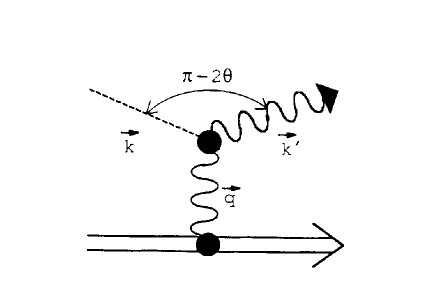
Figure 1: Feynman diagram of the Primakoff conversion of axions into photons.

The terrestrial flux of axions from the sun can be approximated by the expression [7]:

$$\frac{d\Phi}{dE}\;=\;\lambda^{1/2}\,\frac{\Phi_{\rm{}_{o}}(E/E_{\rm o})^{3}}{E_{\rm{}_{o}}(e^{E/E_{\rm o}}\,-\,1)}\;,$$ (1)

where $\lambda=(g_{a\gamma\gamma}\times 10^{8})^{4}$ and is dimensionless, $E_{\rm o}=1.103$ keV, and $\Phi_{\rm o}=5.95\times 10^{14}$ cm^-2 sec^-1. The total flux for $\lambda=1$ integrated from 0 to 12 keV is $3.54\times 10^{15}$ cm^-2 sec^-1. The spectrum is a continuum peaking at about 4 keV decreasing to a negligible contribution above 8 keV. The differential cross section for Primakoff conversion on an atom with nuclear charge $Ze$ is:

$$\frac{d\sigma}{d\Omega}\;=\;\left[\frac{Z^{2}\alpha\hbar^{2}c^{2}g_{a\gamma\gamma}^{2}}{16\pi}\right]\,\frac{q^{2}\,(4k^{2}\,-\,q^{2})}{(q^{2}\,+\,r_{\rm o}^{-2})^{2}}\;,$$ (2)

where $q$ is the momentum transfer, $k$ is the momentum of the incoming axion, and $r_{\rm o}$ is the screening length of the atom in the lattice. For germanium, $\sigma_{\rm o}=Z^{2}\alpha\hbar^{2}c^{2}g_{a\gamma\gamma}/8\pi=1.15\times 10^{-44}$ cm² when $g_{a\gamma\gamma}=10^{-8}$ GeV^-1, or equivalently $\lambda=1$.

For light axions the Primakoff process in a periodic lattice is coherent when the Bragg condition ($2d\sin\theta=n\lambda$) is satisfied, that is when $\vec{q}$ transferred to the crystal is a reciprocal lattice vector $\vec{G}=2\pi(h,k,l)/a_{\rm o}$. Here $a_{\rm o}$ is the size of the conventional cubic cell, and $h$, $k$, and $l$ are integers.

It was shown that the rate of conversion of axions with energy $E$ when the sun is in the direction $\hat{k}$, $\dot{N}(\hat{k},E)$, can be written [2]:

$$\dot{N}(\hat{k},E) = 2\hbar c\,\frac{V}{v_{c}}\,\sum_{G}\left|S(G)\right|^{2}\,\frac{d\sigma}{d\Omega}(\vec{G})\,\frac{1}{|\vec{G}|^{2}}\,\times$$ (3)

$$\hskip 28.45274pt\frac{d\Phi}{dE}\delta(E-\frac{\hbar c|\vec{G}|^{2}}{2\hat{k}\cdot\vec{G}})\;,$$

where $V$ is the volume of the crystal, $v_{c}$ is the volume of a unit cell, $S(G)$ is the structure function for germanium, and $d\Phi/dE$ is evaluated at the axion energy of $\hbar c|\vec{G}|^{2}/2\hat{k}\cdot\vec{G}$. The structure function for germanium is:

$$S(G) = \left[1\,+\,e^{i\pi(h+k+l)/2}\right]\left[1\,+\,e^{i\pi(h+k)}\,+\,\right.$$ (4)

$$\left.e^{i\pi(h+l)}\,+\,e^{i\pi(k+l)}\right]\;.$$

Note that in (3) the coherent conversion of axions occurs only for a particular axion energy given the position of the sun, $\hat{k}$, and reciprocal lattice vector $\vec{G}$. However, the detector has a finite energy resolution; for the detector in Sierra Grande it is 1 keV FWHM at 10 keV. We take this into account by smoothing $\dot{N}(\hat{k},E)$ with a Gaussian of the appropriate width. Finally, we take the relevant part of the energy spectrum, in this case from the threshold energy of 4 keV up to 8 keV (which is just below the X-rays at 10 keV), and calculate the total rate of conversion in windows of width $\Delta E$, typically 0.5 keV,

$$R(\hat{k},E) = 2\hbar c\,\frac{V}{v_{c}}\,\sum_{G}\left|S(G)\right|^{2}\frac{d\sigma}{d\Omega}\,\frac{1}{\left|\vec{G}\right|^{2}}\,\times\hskip 14.22636pt$$ (5)

$$\frac{d\Phi}{dE}\,\frac{1}{2}\left[{\rm erf}\left(\frac{E-E_{a}}{\sqrt{2}\sigma}\right)-{\rm erf}\left(\frac{E-E_{a}-\Delta E}{\sqrt{2}\sigma}\right)\right],$$

where $E_{a}=\hbar c\left|G\right|^{2}/(2\hat{k}\cdot\vec{G})$ and ${\rm erf}(x)=\frac{2}{\sqrt{\pi}}\int_{0}^{x}e^{-t^{2}}dt$ is the error function. In equation (5) we have neglected the angular size of the core of the sun and the mass of the axion which is justified when $m_{a}c^{2}$ is small compared to the core temperature of the sun [5], i.e., up to a few keV.

The theoretical axion detection rate for this detector, calculated with equation (5), is shown in Figure 2. The position of the sun is computed at any instant in time using the U.S. Naval Observatory Subroutines (NOVAS) [8]. The pronounced variation in $R(\hat{k},E)$ as a function of time invites the data to be analyzed with the correlation function:

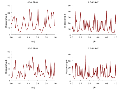
Figure 2: A typical axion-photon conversion rate, $R(t,E)$, for various energy bands. The experimental energy resolution FWHM=1.0 keV at 10 keV was used.

$$\chi\;\equiv\;\sum_{i=1}^{n}\,\left[R(t_{i},E)\;-\,\langle R(E)\rangle\right]\,n(t_{i})\;,$$ (6)

where $R(t_{i},E)$ is the smooth shape of the theoretical rate at the instant of time, $t_{i}$, $\langle R(E)\rangle$ is the average rate over a finite time interval, and $n(t_{i})$ is the number of events at $t_{i}$ in a time interval $\Delta t$, usually 0 or 1. The choice for the weighting function $W(t,E)=R[\hat{k}(t),E]-\langle R(E)\rangle$ is motivated by the requirement that any constant background average to zero in $\chi$, whereas a counting rate which follows $R[\hat{k}(t),E]$ increases $\chi$.

The number of counts at time, $t$, in the interval $\Delta t$ is assumed to be due in part to axions and in part to background governed by a Poisson process with mean:

$$\langle n(t)\rangle\;=\;\left[\lambda\,R(t,E)\,+\,b(E)\right]\,\Delta t,$$ (7)

where $b(E)$ is constant in time.

The average value of $\chi$ is then,

$$\langle\chi\rangle = \sum_{i}\left[R(t_{i},E)\;-\,\langle R(E)\rangle\right]\left[\lambda R(t_{i},E)\,+\,\right.$$ (8)

$$\hskip 56.9055pt\left.b(E)\right]\Delta t$$

$$\;=\; \sum_{i}W(t_{i},E)\left[\lambda R(t_{i},E)+b(E)\right]\,\Delta t.$$

We can add and subtract the constant quantity $\lambda\langle R(E)\rangle$ to the second factor in eq. (8). Any time independent contributions multiplied by $W(t,E)$ in eq. (8), and summed over time, will vanish. Accordingly, taking the limit as $\Delta t\rightarrow 0$, we obtain:

$$\langle\chi(\lambda)\rangle\;=\;\lambda\,\int_{0}^{T}\,W^{2}(t,E)\,dt.$$ (9)

The expected uncertainty in $\chi$, $(\Delta\chi)^{2}=\langle\chi^{2}\rangle-\langle\chi\rangle^{2}$, is given by,

$$(\Delta\chi)^{2} = \sum_{i}\,\sum_{j}\,W(t_{i},E)W(t_{j},E)\,\times$$

$$\left[\langle n(t_{i})n(t_{j})\rangle\,-\,\langle n(t_{i})\rangle\langle n(t_{j})\rangle\right]$$

$$= \sum_{i}W^{2}(t_{i},E)\left[\langle n(t_{i})^{2}\rangle-\langle n(t_{i})\rangle^{2}\right],$$

where the square bracket is $\langle\Delta n(t_{i})\rangle^{2}$, which in Poisson statistics is $\langle n(t_{i})\rangle$. Accordingly,

$$(\Delta\chi)^{2}\;=\;\sum_{i}\,W^{2}(t_{i},E)\langle n(t_{i})\rangle.$$ (11)

By (7) we have:

$$(\Delta\chi)^{2} = \sum_{i}\,W^{2}(t_{i},E)\,\left[\lambda\,R(t_{i},E)\,+\,b(E)\right]\,\Delta t$$ (12)

$$= \sum_{i}W^{2}(t_{i},E)\left\{\lambda\left[R(t_{i},E)-\langle R(E)\rangle\right]\right.$$

$$+\left.\lambda\langle R(E)\rangle+b(E)\right\}\Delta t,$$

which in the limit $\Delta t\rightarrow 0$ becomes,

$$(\Delta\chi)^{2} = \lambda\int_{0}^{T}W^{3}(t,E)dt\,+\,$$ (13)

$$R_{T}(E)\int_{0}^{T}W^{2}(t,E)dt.$$

The quantity $R_{T}(t,E)$ is the average total counting rate, including both axion conversions and background.

The data are separately analyzed in energy bins, $\Delta E_{k}$, fixed by the detector resolution (FWHM $\sim 1$ keV in this case). The likelihood function is then constructed:

$$L(\lambda)\;=\;\prod_{k}\,\exp\left[\frac{-(\chi_{k}\,-\,\langle\chi_{k}\rangle)^{2}}{2(\Delta\chi_{k})^{2}}\right].$$ (14)

To an excellent approximation $(\Delta\chi_{k})^{2}$ is dominated by background. Maximizing the likelihood function, the most probable value of $\lambda$ is given by

$$\lambda_{\rm o}\;=\;\sum_{k}\,\chi_{k}\,/\,\sum_{k}\,A_{k},$$ (15)

where,

$$A_{k}\;\equiv\;\int_{0}^{T}\,W_{k}^{2}(t,E)\,dt,$$ (16)

and the width of the likelihood function is given by,

$$\sigma_{\lambda}\;=\;\left(\sum_{k}\,A_{k}\,/\,b_{k}\right)^{-1/2}.$$ (17)

We note that $A_{k}$ is proportional to the time of the experiment, so that $\sigma_{\lambda}$ decreases as $T^{1/2}$. The background scales with the detector mass, while $A_{k}$ scales as the square of the detector mass, therefore $\sigma_{\lambda}$ decreases as $(M_{d}T)^{-1/2}$.

We have carried out extensive Monte-Carlo test of this method of analysis. As a test of our analysis, typical results for the likelihood function for the cases $\lambda=0$ (no axions) and $\lambda=0.003$ were calculated with realistic backgrounds for a detector operating with the same mass, energy resolution, and threshold as the DEMOS detector at the latitude and longitude of Sierra Grande for one year. It is clear from this calculation that the correlation function analysis is consistent and quite sensitive to the presence of a variation in the counting range due to solar axions with a signal to noise ratio less than 1%.

The vertical axis of our detector is the (100) crystalline axis. The orientation of the (010) and (001) axes are unknown at this time. Therefore, to place a bound on the axion interaction rate, the data must be analyzed for many azimuthal orientations of the crystal, and the weakest bound selected. The results of these calculations for 707 days of data in the energy range from 4 to 8 keV in 0.5 keV intervals are shown in Figure 3.

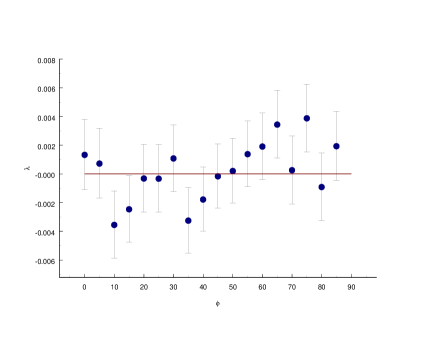
Figure 3: Values of $\lambda$ calculated from the 707 days of data as a function of the azimuthal angle $\phi$. The error bars are $1\sigma$.

The most conservative upper bound on $\lambda$, or equivalently $g_{a\gamma\gamma}$, is found by taking for $\phi$ the angle at which $\lambda$ is maximum. This yields an upper bound on the axion–photon coupling constant $g_{a\gamma\gamma}<2.7\times 10^{-9}$ GeV^-1 at the 95% confidence level.

In Figure 4 we show the area of the axion mass – coupling constant plane excluded by this result along with results of earlier work.

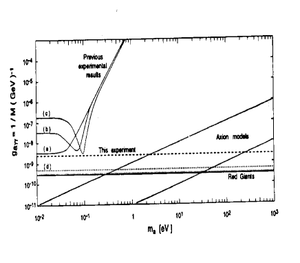
Figure 4: Exclusion plots on the $g_{a\gamma\gamma}$ vs. axion–mass plane. The curve to the left are from Ref. [10]. The letters indicate the following helium gas pressures in the conversion region of a strong magnetic field: (a) vacuum, (b) 55 Torr, and (c) 100 Torr.

While this bound is interesting because it is a laboratory constraint, it does not challenge the bound placed by Raffelt [9], $g_{a\gamma\gamma}\leq 10^{-10}$ GeV^-1 based on the helium burning rate in low mass stars. A coupling constant $g_{a\gamma\gamma}\simeq 10^{-9}$ GeV^-1 would imply axion emission rates 100 times higher than the stellar bound, and a significantly different concept of stellar evolution.

This experiment can be considerably improved by using a large number of smaller p–type germanium detectors with known orientations of the (010) axes, with energy thresholds below 2 keV, and energy resolutions corresponding to FWHM $\approx$ 0.5 keV. This is being proposed at this time. Another collaboration could also operate the COSME experiment in the new University of Zaragoza underground laboratory in the Canfranc tunnel at 42^o 48’ N and 0^o 31’ W. The COSME detector is a 0.25 kg crystal having an energy threshold of $\sim$1.8 keV and a resolution of 0.5 keV FWHM at 10 keV. A positive result in this northern hemisphere experiment over a wider energy range should have a very different temporal pattern from that of the Sierra Grande experiment, but should yield the same value of $\lambda$.

One of the USC/PNNL twin detectors is currently operating in the Baksan Neutrino Observatory in Russia at 660 mwe, and if moved to a location with greater overburden could also be used to acquire meaningful data on solar axion rates.

The analysis presented here allows one to legitimately combine the results of a number of experiments. Accordingly, the results from a large number of experiments located throughout the world can be combined to yield results equivalent to a single large experiment.

References

- [1] R. D. Peccei and H. Quinn, Phys. Rev. Lett. 38 (1977) 1440; Phys. Rev. Dl6 (1977) 1791.
- [2] R. J. Creswick, F. T. Avignone III, H. A. Farach, J. I. Collar, A. O. Gattone, S. Nussinov, and K. Zioutas, (Submitted to Phys. Lett. 1997).
- [3] D. E. Di Gregorio, D. Abriola, F. T. Avignone III, R. L. Brodzinski, J. I. Collar, H. A. Farach, E. García, A. O. Gattone, F. Hasenbalg, H. Huck, H. S. Miley, A. Morales, J. Morales, A. Ortiz de Solórzano, J. Puimedón, J. H. Reeves, C. Sáenz, A. Salinas, M. L. Sarsa, D. Tomasi, I. Urteaga, and J. A. Villar, Nucl. Phys. B (Proc. Suppl.) 48 (1996) 56
- [4] D. Abriola, F. T. Avignone III, R. L. Brodzinski, J. I. Collar, D. E. Di Gregorio, H. A. Farach, E. García, A. O. Gattone, F. Hasenbalg, H. Huck, H. S. Miley, A. Morales, J. Morales, A. Ortiz de Solórzano, J. Puimedón, J. H. Reeves, C. Sáenz, A. Salinas, M. L. Sarsa, D. Tomasi, I. Urteaga, and J. A. Villar, Astropart. Phys. 6 (1996) 63.
- [5] W. Buchmüller and F. Hoogeveen, Phys. Lett. B237 (1990) 278.
- [6] E. A. Paschos and K. Zioutas, Phys. Lett. B323 (1994) 367.
- [7] K. van Bibber, P. M. McIntyre, D. E. Morris, G. G. Raffelt, Phys. Rev. D39 (1989) 2089.
- [8] G. H. Kaplan, J. A. Huges, P. K. Seidelmann, C. A. Smith, and B. D. Yallop, Astronomical Journal 97 (1989) 1197.
- [9] G. G. Raffelt, Phys. Reports 198 (1990) 1.
- [10] D. M. Lazarus, G. C. Smith, R. Cameron, A. C. Melissinos, G. Ruoso, Y. K. Semertzidis, and F. A. Nezrick. Phys. Rev. Lett. 69 (1992) 2333.