AGAPEROS: Searching for microlensing in the LMC with the Pixel Method

Abstract

Recent surveys monitoring millions of light curves of resolved stars in the LMC have discovered several microlensing events. Unresolved stars could however significantly contribute to the microlensing rate towards the LMC. Monitoring pixels, as opposed to individual stars, should be able to detect stellar variability as a variation of the pixel flux. We present a first application of this new type of analysis (Pixel Method) to the LMC Bar. We describe the complete procedure applied to the EROS 91-92 data (one tenth of the existing CCD data set) in order to monitor pixel fluxes. First, geometric and photometric alignments are applied to each images. Averaging the images of each night reduces significantly the noise level. Second, one light curve for each of the $2.1\times 10^{6}$ pixels is built and pixels are lumped into 3.6$\arcsec\times$ 3.6$\arcsec$ super-pixels, one for each elementary pixel. An empirical correction is then applied to account for seeing variations. We find that the final super-pixel light curves fluctuate at a level of 1.8% of the flux in blue and 1.3% in red. We show that this noise level corresponds to about twice the expected photon noise and confirms previous assumptions used for the estimation of the contribution of unresolved stars. We also demonstrate our ability to correct very efficiently for seeing variations affecting each pixel flux. The technical results emphasised here show the efficacy of the Pixel Method and allow us to study luminosity variations due to possible microlensing events and variable stars in two companion papers.

1 Introduction

The amount and nature of Dark Matter present in the Universe is an important question for cosmology (see e.g. White et al. (1996) for current status). On galactic scales (Ashman 1992), dynamical studies (Zaritsky 1992) as well as macrolensing analyses (Carollo et al. 1995) show that up to 90% of the galactic masses might not be visible. One plausible explanation is that the stellar content of galaxies is embedded in a dark halo. Primordial nucleosynthesis (Walker et al. 1991; Copi et al. 1995) predicts a larger number of baryons than what is seen (Persic & Salucci 1992), and so dark baryons hidden in gaseous or compact objects (Carr 1994, Gerhard & Silk 1996) could explain, at least in part, the dark galactic haloes.

In 1986, Paczyński proposed microlensing techniques for measuring the abundance of compact objects in galactic haloes. The LMC stars are favourable targets for microlensing events searches. Since 1990 and 1992, the EROS (Aubourg et al. 1993) and MACHO (Alcock et al. 1993) groups have studied this line of sight. The detection of 10 microlensing events has been claimed in the large mass range $0.05-1M_{\odot}$ (Aubourg et al. 1993, Alcock et al. 1996). This detection rate, smaller than expected with a full halo, indicates that the most likely fraction of compact objects in the dark halo is $f=0.5$ (Alcock et al. 1996). Concurrently, the small mass range has been excluded for a wide range of galactic models by the EROS and MACHO groups. Objects in the mass range ($5\times 10^{-7}M_{\odot}<M<5\times 10^{-4}M_{\odot}$) could not account for more than 20% of the standard halo mass (Alcock et al. 1998). In the meantime, the DUO (Alard et al. 1995), MACHO (Alcock et al. 1995) and OGLE (Udalski et al. 1995) groups look towards the galactic bulge where star-star events are expected. The detection rate is higher than expected from galactic models (see for instance Evans 1994, Alcock et al. 1995, Stanek et al. 1997). The events detected in these two directions demonstrate the efficacy of the microlensing techniques based on the monitoring of several millions of stars.

Microlensing Searches with the Pixel Method

The detection of a larger number of events is one of the big challenges in microlensing searches. This basically requires the monitoring of a larger number of stars. The Pixel Method, initially presented by Baillon et al. (1993), gives a new answer to this problem: monitoring pixel fluxes. On images of galaxies, most of the pixel fluxes come from unresolved stars, which contribute to the background flux. If one of these stars is magnified by microlensing, the pixel flux will vary proportionally. Such a luminosity variation can be detected above a given threshold, provided the magnification is large enough. Unlike other approaches (namely star monitoring and Differential Image Photometry, see below), the Pixel Method does not perform a photometry of the stars but is designed to achieve a high efficiency for the detection of luminosity variations affecting unresolved stars. This means that we will work with pixel fluxes and not with star fluxes. A theoretical study of the pixel lensing method has been published by Gould (1996b).

This pixel monitoring approach has two types of application. Firstly, it allows us to investigate more distant galaxies and thus to study other lines of sight. This has led to observations of the M31 galaxy. The AGAPE team (Ansari et al. 1997) has shown that this method works on M31 data, and luminosity variations compatible with the expected microlensing events have been detected but the complete analysis is still in progress (Giraud-Héraud 1997). A similar approach, though technically different, called Differential Image Photometry is also investigated by the VATT/Columbia collaboration (Crotts 1992, Tomaney & Crotts 1996). Some prospective work has also been done towards M87 (Gould 1995).

The second possibility is to apply pixel microlensing on existing data, thus extending the sensitivity of previous analyses to unresolved stars. This is precisely the subject of this paper and of the two which will follow: we present the implementation of the Pixel Method on CCD images of the LMC.

Pixel Method on the LMC

We have applied for the first time a comprehensive pixel analysis on existing LMC images collected by the EROS collaboration. With respect to previous analyses (Queinnec 1994, Aubourg et al. 1995, Renault 1996), our analysis of the same data using pixel monitoring allows us to extend the mass range of interest up to $1\,M_{\odot}$ and to increase the sensitivity of microlensing searches. On these images, a large fraction of the stars remains unresolved: typically 5 to 10 stars contribute to 95% of the pixel flux in one square arc-second. Since this approach potentially uses all the image content (and not only the resolved stars), the volume of the data to handle is much larger. Hence we perform this first exploratory analysis on a relatively small data set: 0.25 deg² covering a period of observation of 120 days, which corresponds to 10% of the LMC CCD data (91-94).

This paper is the first of a series of three, describing the data treatment (this paper), the microlensing search (Melchior et al. 1998a, hereafter Paper II) and a catalogue of variable stars (Melchior et al. 1998b, hereafter Paper III). In the companion papers (Papers II and III), we show how the data treatment described here to produce pixel light curves allows us to perform analyses that increase the sensitivity to microlensing events and variable stars with respect to the star monitoring analysis applied on the same field: an order of magnitude in the number of detectable luminosity variations is gained.

To discover real variations, the images and light curves have to be corrected for various sources of fake variabilities, such as geometrical and photometric mismatch, or seeing changes between successive images. The construction of light curves cleaned from these effects is the subject of this first paper. If the flux of a given star contributes to the pixel flux, the latter can be expressed as follows:

$$\phi_{pixel}=f\times\phi_{\rm star}+\phi_{bg},$$ (1)

where $\phi_{\rm star}$ is the flux of the given star, $f$ the fraction of the star flux that enters the pixel, hereafter called seeing fraction and $\phi_{bg}$ corresponds to the flux of all other contributing stars plus the sky background.

If this particular star exhibits a luminosity variation, then we will be able to detect it as a variation of the pixel flux:

$$\Delta\phi_{pixel}=f\times\Delta\phi_{\rm star},$$ (2)

provided it stands well above the noise. Actually, this pixel flux is affected by the variations of the observational conditions and our goal here is to correct for them. We discuss the level of noise achieved after these corrections and include this residual noise in error bars. The outline of this paper is as follows. In Sect. 2, we start with a short description of the data used. In Sect. 3, we successively describe the geometric and photometric alignments applied to the images. We are thus able to build pixel light curves and to discuss their stability after this preliminary operation. In Sect. 4, we average the images of each night, thus reducing the fluctuations due to noise considerably. In Sect. 5, we consider the benefits of using super-pixel light curves. In Sect. 6, we correct for seeing variations and obtain light curves cleaned from most of the changes in the observational conditions. At this stage, a level of fluctuations smaller than 2% is typically achieved on the super-pixel fluxes. In order to account for the noise present on the light curves, we estimate, in Sect. 7, an error for each super-pixel flux. We conclude in Sect. 8 that the light curves of super-pixels, resulting from the complete treatment, reach the level of stability close to the expected photon noise. They are therefore ready to be used to search for microlensing events and variable objects, as presented in the companion Papers II and III.

2 The data

2.1 Description of the data set

The data have been collected at La Silla ESO in Chile with a $40$cm telescope ($f/10$) equipped with a thick CCD camera composed of $8\times 2$ CCD chips of $400\times 579$ pixels with scale of $1.21\arcsec$/pixel (Arnaud et al., 1994b, Queinnec, 1994 and Aubourg et al., 1995). The gain of the camera was $6.8{e^{-}}/$ADU with a read-out noise of 12 photo-electrons. For the 1991-92 campaign only 11 chips out of 16 were active. Due to technical problems, we only analyse 10 of them. The monitoring has been performed in two wide colour bands (Arnaud et al., 1994a). Exposure times were set to 8 min in red ($\langle{\lambda}\rangle=670$ nm) and 15 min in blue ($\langle{\lambda}\rangle=490$ nm). As the initial goal was to study microlensing events with a short-time scale (Aubourg et al. 1995), up to 20 images per night in both colours are available. A total of 2000 blue and red images were collected during 95 nights spread over a 120 days period (18 December 1991 - 11 April 1992). The combined CCD and filter efficiency curves as shown in Grison et al. (1995) lie below 15% in blue and below 35% in red. Bias subtraction and flat-fielding have been performed on-line by the EROS group.

The seeing varies between $1.6$ and $3.6$ arc-second with a mean value of $2.9$ arc-second (typical dispersion $0.5$ arc-second). It should be emphasised that the observational strategy (exposure time) has been optimised for star monitoring. In other words, this means that the photon noise associated with the mean flux (typically 280 ADU per pixel in red and 100 ADU in blue) is relatively large: 6.6 ADU in red and 3.8 ADU in blue. To apply the Pixel Method to this data set, we take advantage of the large number of images available per night, increasing the signal-to-noise ratio with an averaging procedure.

2.2 Absolute calibration

The procedures described below are performed with respect to a reference image. The correspondence between the flux measured on these images and the magnitude, deduced from Grison et al (1995), is as follows:

$$m_{B}=-2.5\log\phi_{B}+24.8$$ (3)

$$m_{R}=-2.5\log\phi_{R}+24.9$$ (4)

where $\phi_{B}$ and $\phi_{R}$ are the flux of a star in ADU in the blue and red respectively. Note that the zero point is about the same in the two colours, whereas the background flux is much larger in red than in blue. The correspondence with the Johnson-Cousins system can be found in Grison et al. (1995).

The aim of the whole treatment presented below is to obtain pixel light curves properly corrected for variations of the observational conditions. The PEIDA package used by the EROS group was adapted for pixel monitoring. This treatment is applied to the first CCD campaign (1991-92) of the EROS group on the LMC bar, i.e. 10% of the whole data set analysed in Renault (1996).

3 Image alignments

The alignments described in this section are needed in order to build pixel light curves from images that are never taken under the same observing conditions. Firstly, the telescope never points exactly twice in the same direction so that the geometric alignment must ensure that the same area of the LMC contributes to the same pixel flux, through the entire period of observation. Secondly, photometric conditions, atmospheric absorption and sky background light change from one frame to another. The photometric alignment corrects for these global variations.

Errors affecting pixel fluxes after these corrections are a key issue as discussed through this section. It is not obvious how to disentangle the various sources of error introduced at each step, in particular after the geometric alignment. Global errors for each pixel flux, including all sources of noise, will be evaluated in Sect. 7.

3.1 Geometric alignment

Between exposures, images are shifted by as much as 40 pixels and this displacement has to be corrected, in order to ensure that each pixel always covers the same area of the LMC. As emphasised below, errors affect the pixel flux after the geometric alignment and two components can be distinguished. The first one, resulting from the uncertainty in the parameters of displacement, turns out to be negligible, whereas the second one, introduced by the linear interpolation, is a more important source of noise. In this sub-section, we give a qualitative overview of these sources of errors. This study, based on synthetic images, allows us to disentangle errors due to the geometrical alignment from other effects present on real images, because the position and content of unaligned synthetic frames are known by construction.

Displacement parameters.

The parameters of displacement are determined with the PEIDA algorithm (Ansari, 1994), based on the matching of star positions. Beside translation, rotation and dilatation are also taken into account as far as their amplitude remains small (otherwise the corresponding images are removed from further consideration).

A series of mock images synthesised with the parameters of real images (geometric displacement, absorption, sky background and seeing) allows us to estimate the mean error on the pixel position to be $0.011\pm 0.005$ pixel. Similar estimates have been obtained by the EROS group (Ansari, private communication) on real data.

This introduces a small mismatch between pixel fluxes: in first approximation, the error on the flux is proportional to the pixel area corresponding to the difference between the true and the computed pixel position.

Linear interpolation.

Once the parameters of displacement are estimated, pixel fluxes are corrected with a linear interpolation. This interpolation is necessary in order to monitor pixel fluxes, and to build pixel light curves.

Figure 1: Error due to linear interpolation estimated with two sets of synthetic images: $\sigma$ is the dispersion measured on the flux difference between pixels on the “reference” image and corrected images, while $v$ is a function of the displacement, as discussed in the text (Eq. 5).

We use synthetic images to understand qualitatively the residual errors. Two sets of blue images are simulated with the identical fluxes (new moon condition) and seeings (2.5 arc-second) but shifted with respect to one of them (the “reference” image). A linear interpolation is applied to each of these images in order to match the position of the reference. In case of pure translation, the corrected flux is computed with the flux of the 4 pixels overlapping the pixel $p$ on the reference frame: the areas of these intersections with this pixel $p$ are used to weight each pixel flux. The square of the variable $v$, depending upon $\delta x$ and $\delta y$, the displacement in the $x$ and $y$ directions,

$$v=\sqrt{\left(\delta x^{2}+{\left(1-\delta x\right)}^{2}\right)\left(\delta y^{2}+{\left(1-\delta y\right)}^{2}\right)},$$ (5)

is the sum of the square of these overlapping surfaces. It characterises the mixing of pixel fluxes produced by this interpolation: the smaller $v$ is, the more pixels are mixed by the interpolation.

Figure 1 displays an estimate of the residual errors affecting pixel fluxes for different displacement parameters, and shows a correlation of the errors with the variable $v$. The first set of images, simulated without photon noise, shows errors on pixel fluxes due to linear interpolation smaller than 5.5 ADU (about 4.5% of the mean flux). The second set of images, simulated with photon noise, allows us to check that the photon noise adds quadratically with the “interpolation” noise and that residual errors are smaller than 7 ADU. The correlation observed on this figure between the error $\sigma$ and the variable $v$ can be understood as follows: when $v$ decreases, the interpolated image gets more and more degraded, and the interpolation noise increases while the poisson noise is smeared out.

This residual error is strongly seeing dependent. If the above operation is performed on an image with a seeing of $2$ arc-second, the residual errors are as large as 10% of the mean flux: the larger the seeing difference, the larger the residual error. As the seeing of raw images varies between $1.6$ and $3.6$ arc-second, this makes a detailed error tracing very difficult. The PSF is also slightly widened due to the re-sampling, but this effect remains small compared to other sources of PSF variability, and is largely averaged out when summing over the images of a night (see Sect. 4).

3.2 Photometric alignment

Figure 2: Photometric alignment: (a) absorption and (b) sky background flux (in ADU) estimated in each blue image.

Changes in observational conditions (atmospheric absorption and background flux) are taken into account with a global correction relative to the reference image. We assume that a linear correction is sufficient:

$$\phi_{\rm corrected}=a\phi_{raw}+b,$$ (6)

where $\phi_{\rm corrected}$ and $\phi_{raw}$ are the pixel fluxes after and before correction respectively. The absorption factor $a$ is estimated for each image with a PEIDA procedure, based on the comparison of star fluxes between this image and the reference frame (Ansari, 1994). A sky background excess is supposed to affect pixel fluxes by an additional term $b$ which differs from one image to another.

In Fig. 2, we plot the absorption factor (top) and the sky background (bottom) estimated for each image with respect to the reference image as a function of time. The absorption can vary by as much as a factor $2$ within a single night. During full moon periods, the background flux can be up to 20 times higher than during moonless nights, increasing the statistical fluctuations by a factor up to 4.5. However, this high level of noise concerns very few images (see Fig. 2), and only about 20% of the images more than double their statistical fluctuations. Despite their large noise, full moon images improve the time sampling, and at the end of the whole treatment, the error bars associated with these points are not significantly larger than those corresponding to new moon periods, except for a few nights.

3.3 Residual large-scale variations and their correction

We note the presence of a variable spatial pattern particularly important during full moon periods. This residual effect, probably due to reflected light, can be eliminated with a procedure similar to that applied to the AGAPE data, as described by Ansari et al. (1997). We calculate a median image with a sliding window of $9\times 9$ pixels on the difference between each image and the reference image. It is important to work on the difference in order to eliminate the disturbing contributions of stars, and to get a median that retains only large-scale spatial variations. We then subtract the corresponding median from each image, to filter out large-scale spatial variations. In Fig. 3, we show a light curve before and after this correction. Above, the pixel light curve presents important systematic effects during full moon periods, effects which have disappeared below, after correcting for these large-scale variations.

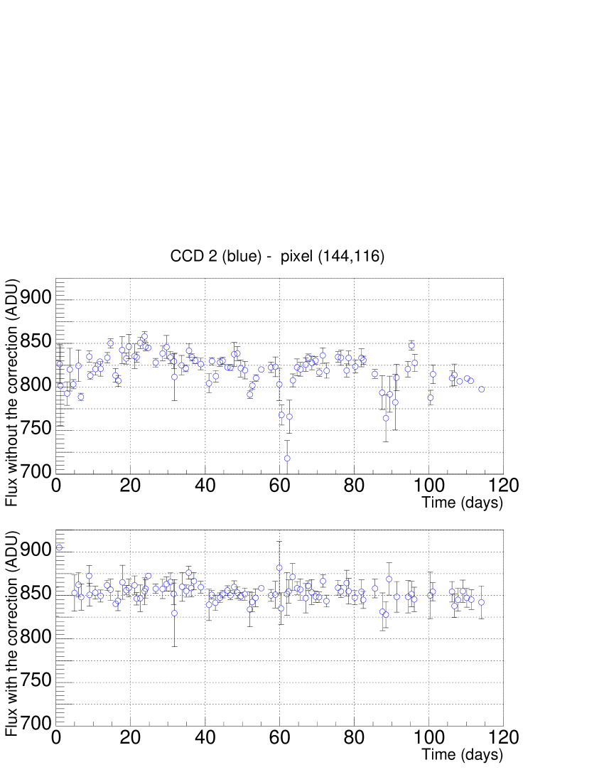
Figure 3: Pixel light curve before (above) and after (below) filtering out the large-scale spatial variations. Fluxes are given in ADU.

3.4 Image selection

After these alignments, we eliminate images whose parameters lie in extreme ranges. We keep images which have no obvious defects and parameters in the following range:

• Absorption factor:
  $0.6<a^{R}<1.5$ ; $0.6<a^{B}<1.5$

• Mean flux (ADU):
  $100.0<\phi^{R}<2000.0$
  $70.0<\phi^{B}<1500.0$

• Seeing (arcsec):
  $S^{R}<3.6$ ; $S^{B}<3.6$

This procedure rejects about 33% of the data.

3.5 Stability of elementary pixels after alignment

Figure 4: Relative flux stability of about 1000 flux measurements in the blue band, spread over 120 days for pixels within a $50\times 50$ patch of CCD 3.

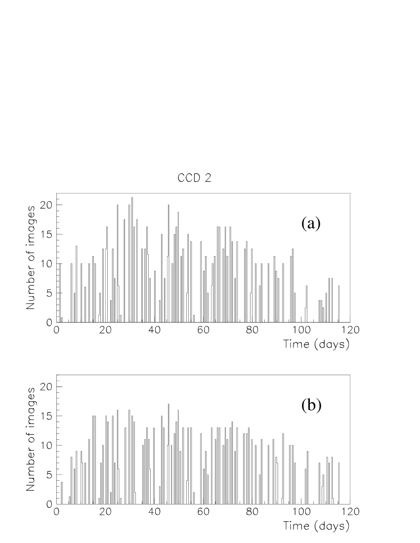
Figure 5: Number of images per night for one CCD field: in red (a) and in blue (b).

We are now able to build pixel light curves, made of about 1000 measurements spread over 120 days. The stability can be expressed in term of the relative dispersion ${\sigma}/{\phi}$ measured for each light curve, where $\phi$ stands for the mean flux and $\sigma$ for the dispersion of the light curve. This dispersion gives us a global estimate of the errors introduced by the alignments, combined with all other sources of noise (photon noise, read-out noise…). In Fig. 4, we present the histogram of this dispersion for one $50\times 50$ patch of one CCD field, which shows a mean dispersion of 9.1%. We estimate the contribution of the photon noise alone to be as high as 7%. With such a noise level, dominated at this stage by photon counting and flux interpolation errors, one does not expect a good sensitivity to luminosity variations. Fortunately, various improvements described in the following (namely the averaging of the images of each night, the super-pixels and the seeing correction) will further reduce this dispersion by a factor of 5.

4 Going to one image per night

Figure 6: A stable pixel light curve (a) before and (b) after the mean is performed over each night.

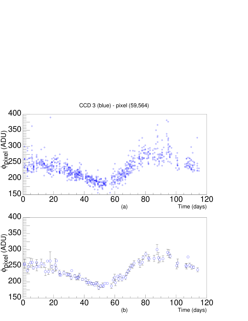
Figure 7: A variable pixel light curve before (a) and after (b) the mean is performed over each night.

The motivation of this pixel analysis is to increase the sensitivity to long duration events ($\geq 5$ days) in the mass range where all the known candidates have been observed. It is crucial to note that a sampling rate of 1 measurement per day is sufficient. The numerous images available each night (up to 20 per night) allow us to reduce the noise discussed in Sect. 3.5, by co-adding them, and are very useful for the error estimation as emphasised in Sect. 7.

4.1 Construction

We average the images of each night. During the night $n$, we have, for each pixel $p$, $N^{p}_{n}$ measurements of flux ($\phi^{p}_{n,j}$; $j=1,N^{p}_{n}$). The number of measurements $N^{p}_{n}$ available each night is shown in Fig. 5 and ranges between 1 and 20 with an average of 10. The mean flux $\phi^{p}_{n}$ of pixel $p$ over the night is computed removing the fluxes which deviate by more than $3\sigma$ from the mean, in order to eliminate any large fluctuation due to cosmic rays, as well as CCD defects and border effects. Note that, due to this cut-off, the number of measurements $N^{p}_{n}$ used for a given night can differ from pixel to pixel.

Figure 8: Relative flux stability achieved on pixel light curves after averaging the images of each night, on a $50\times 50$ patch of CCD 3.

4.2 Results

Figure 6 shows the result of this operation on a typical pixel light curve. The dispersion in the data on the top panel (a) is reduced and included in the error bars (see in Sect. 7) as shown on the bottom panel (b). Figure 7 shows the same operation applied to a pixel light curve exhibiting a long time scale variation. One can notice that uncertainties in the data during full moon periods are not systematically larger than those corresponding to new moon periods. Figure 8 displays the histogram of relative stability for the resulting light curves, for the same area as for Fig. 4. A mean dispersion of 3.9% is measured: the noise is thus reduced by more than a factor 2. Photon noise is estimated to be 3.3%.

4.3 Additional remarks

Thanks to this procedure the PSF of the composite images will tend towards a Gaussian. This thus removes the inhomogeneity in the PSF shape that can be observed on raw images. In particular, the seeing on these composite images becomes more homogeneous with an average value of $3.0$ arc-second in red and $2.9$ arc-second in blue and a quite small dispersion of 0.25 arc-second. The seeing dispersion is divided by a factor 2 with respect to the initial individual images, whereas the average value is similar.

To summarise, this procedure improves the image quality, reduces the fluctuations that could come from the alignments and removes cosmic rays.

5 Super-pixel light curves

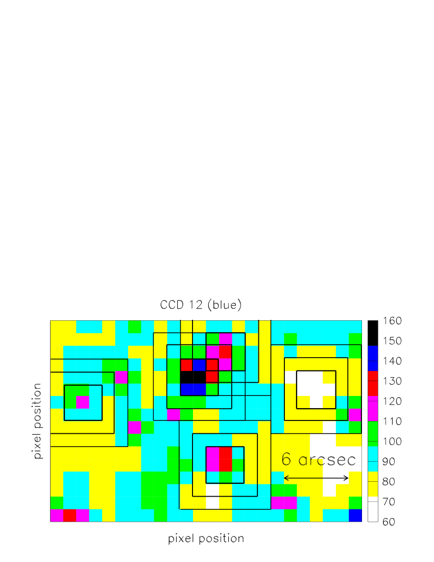
Figure 9: Example of a 19”$\times$29” field on our data in blue, with 3 arcsec seeing. The grey scale gives the intensity in ADU.

Figure 10: The signal to noise ratio expected for a single star, whose centroid lies in the central pixel, is given as a function of the seeing values for different super-pixel sizes. This assumes a circular Gaussian PSF.

So far we have worked with elementary pixel light curves. Pixels which cover 1.21”$\times$1.21” are much smaller than the typical seeing spot and receive on average only 20% of the flux of a star, whose centre lies in the pixel. A significant improvement on the light curves stability can be further achieved by considering super-pixel light curves. Super-pixels are constructed with a running window of $d_{sp}\times d_{sp}$ pixels, keeping as many super-pixels as there are pixels, and their flux is the sum of the $d_{sp}^{2}$ pixel fluxes. These super-pixels have to be taken large enough to encompass most of the flux of a centred star, but not too large in order to avoid surrounding contaminants and dilution. As such, their size should be optimised for this dense star field given the seeing conditions.

Figure 9 illustrates the different super-pixel sizes that can be considered. The expected signal to noise (S/N) ratio is proportional to the ratio of the seeing fraction to the super-pixel size ($d_{sp}$). Going from $1\times 1$ to $3\times 3$ super-pixels increases the seeing fraction by more than a factor 3. Then increasing the super-pixel size further increases the seeing fraction substantially less than the fluctuations of the sky background. Figure 10 displays the variation with seeing of the signal to noise ratio for different super-pixel sizes. It is clear that $3\times 3$ super-pixels offer the best S/N ratio for our configuration.

Figure 11: Flux stability achieved on super-pixel light curves in blue (a) and in red (b) for all the pixels of CCD 3 (before the seeing correction).

As discussed by Ansari et al (1997), the alternative that consists in taking the average of the neighbouring pixels weighted with the PSF is not appropriate here, as it amplifies the fluctuations due to seeing variations.

Figure 11 shows the relative dispersion affecting the super-pixel fluxes for CCD 3: we measure in average 2.1% in blue and 1.6% in red, which corresponds to about twice the estimated level of photon noise (1.1% in blue and 0.7% in red). The comparison with Fig. 8 shows that the dispersion is reduced by a factor smaller than $\sqrt{9\,{\rm(pixels)}}=3$ because of the correlation between neighbouring pixels. This stability can be improved even further by correcting for seeing variations.

6 Seeing correction

Despite of the stability discussed above, fluctuations of super-pixel fluxes due to seeing variations are still present. For a star lying in the central pixel (of the $3\times 3$ super-pixel), on average 70% of the star flux enters on average the super-pixel for a Gaussian PSF, but this seeing fraction is correlated with the changing seeing. In this sub-section, we show that this correlation is linear and can be largely corrected for.

6.1 Correlation between flux and seeing

Depending on their position with respect to the nearest star, super-pixel fluxes can significantly anti-correlate with the seeing if the super-pixel is in the seeing spot, or correlate if instead it lies in the tail of a star.

Figure 12: Histogram of the correlation coefficient $\rho$ between the super-pixel flux and the seeing (before seeing correction).

A correlation coefficient for each super-pixel $p$ can be defined using the usual formula:

$$\rho^{p}=\frac{\sum_{n}\left(\phi^{p}_{n}-\phi\right)\left(S_{n}-S\right)}{\sqrt{\sum_{n}\left(\phi^{p}_{n}-\phi\right)^{2}\sum_{n}\left(S_{n}-S\right)^{2}}}$$ (7)

where $\phi$ and $S$ are the mean values of the super-pixel flux $\phi^{p}_{n}$ and seeing $S_{n}$ on night $n$. In Fig. 12, we show the distributions of correlation coefficients $\rho^{p}$ in blue (left) and in red (right) for each super-pixel $p$. These histograms look quite different in both colours but both distributions have a peak around $\rho\simeq-0.8$. This peak, which corresponds to the anti-correlation with seeing near the centre of resolved stars, is expected due to the large number of resolved stars. It is higher in red than in blue, which is consistent with the EROS colour-magnitude diagram where most detected stars have $B-R>0$ (Renault 1996). The correlation with seeing expected for star tails ($\rho>0$) is less apparent. However, a clear excess at high values of $\rho$ (around $\rho\simeq 0.6$) appears in red, again consistent with the EROS colour-magnitude diagram. Figure 13 gives an example of such a correlation. The upper left panel of Fig. 13 displays the scatter diagram of one super-pixel flux versus the seeing, corresponding to a correlation coefficient $\rho^{p}=-0.89$. Despite the intrinsic dispersion of the measurements (which could be large in particular when a temporal variation occurs), a linear relationship is observed. The bottom left panel displays the light curve of this super-pixel.

Figure 13: Seeing correction applied to the flux of one super-pixel light curve anti-correlated with the seeing ($\rho^{p}=-0.89$). This corresponds to the super-pixel dominated by a centred resolved star, whose position on the CCD frame is labelled “A” in Fig. 15. The error bars shown here and in the following figures are computed as described in Sect. 7.

6.2 Correction

Figure 14: Variation of the seeing fraction of the star flux that enters a $3\times 3$ super-pixel as a function of seeing, for different star positions, given on the figures in pixel unit with respect to the centre of the super-pixel. Panel (a) shows cases when the centre of the star lies within the super-pixel (anti-correlation). Panel (b) shows the seeing fraction that could contribute from surrounding stars (correlation).

This seeing correction is aimed at eliminating the effect of the seeing variations and to obtain pixel light curves that can be described as the sum of a constant fraction of a centred star flux and the background (see Eq. 1). The variation of the super-pixel flux can be interpreted as a variation of the flux of this centred stars (see Eq. 2). However it is clear that the super-pixel flux contains the flux of several stars and that we are not doing stellar photometry, but rather super-pixel photometry.

The idea is to correct for the behaviour described in Sect. 6.1 using a linear expression:

$${{\phi}^{p}_{n}}|_{\rm corrected}=\phi^{p}_{n}-\alpha^{p}\left({S_{n}-S}\right),$$ (8)

where $\alpha^{p}$ is the estimate of the slope for each super-pixel and ${{\phi}^{p}_{n}}|_{\rm corrected}$ is the corrected flux. In the following, $\phi^{p}_{n}$ will stand for this corrected flux.

Figure 14 shows that the seeing fraction of a given star varies linearly with seeing, and hence justifies this correction.

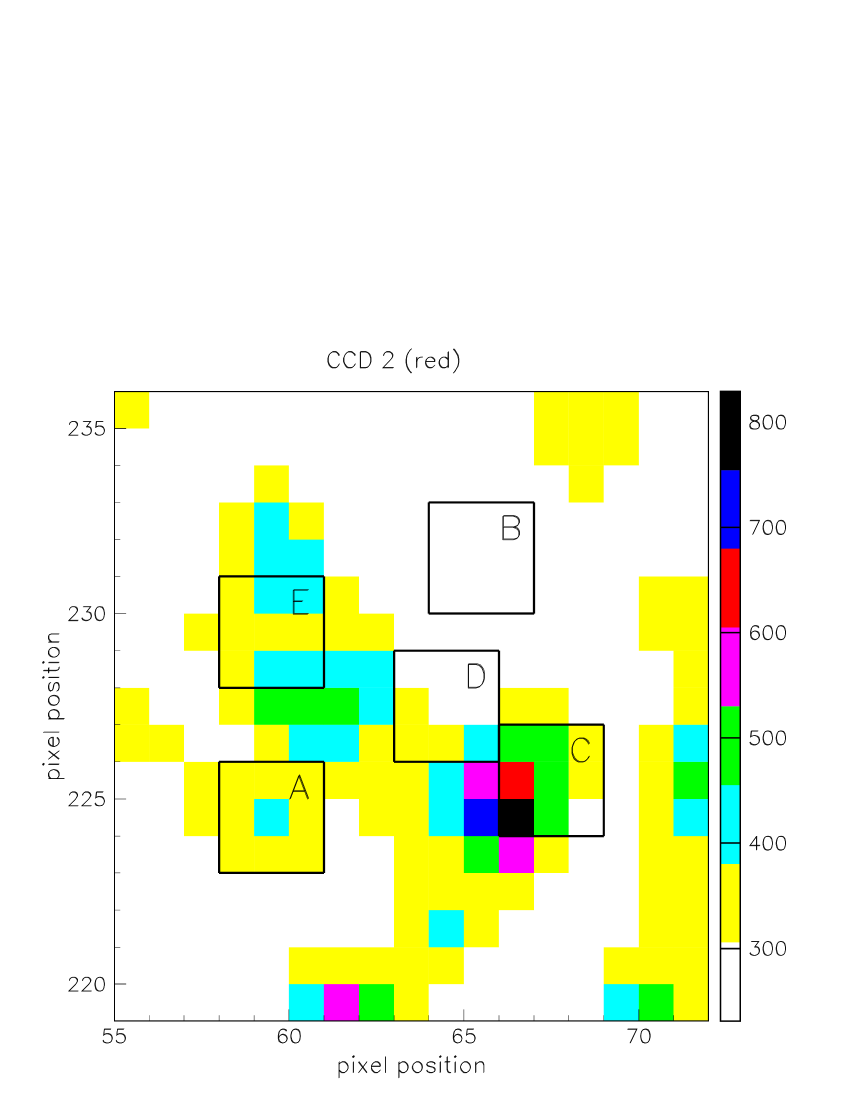
Figure 15: Different super-pixels labelled “A”, “B”, “C”. “D” and “E” corresponding to the different configurations discussed in the text.

Figure 16: Seeing correction applied to the flux of a super-pixel light curve with no significant correlation with the seeing ($\rho^{p}=0.02$). The position of the super-pixel on the CCD frame is labelled “B” in Fig. 15. The stars whose centres lie in the super-pixel are too dim to be resolved.

Figure 17: Seeing correction applied to the flux of a super-pixel light curve strongly anti-correlated with the seeing ($\rho^{p}=-0.94$). The position of the super-pixel on the CCD frame is labelled “C” in Fig. 15. This is a case of blending.

Figure 18: Seeing correction applied to the flux of a super-pixel light curve strongly correlated with the seeing ($\rho^{p}=0.96$). The position of the super-pixel on the CCD frame is labelled “D” in Fig. 15. The super-pixel flux is dominated by tails of surrounding stars. Centred stars are too dim to be resolved.

Figure 19: Seeing correction applied to the flux of a super-pixel light curve not correlated with the seeing ($\rho^{p}=0.05$). The position of the super-pixel on the CCD frame is labelled “E” in Fig. 15. Contributions due to the surrounding stars cancel each other.

If several stars contribute to the super-pixel flux, their contribution will add up linearly, because the flux of the background $\phi_{bg}$ (Eq. 1) can be written as:

$$\phi_{bg}=\sum_{i=1}^{N^{\rm other}_{\rm stars}}f_{i}\phi_{i}+\phi^{\rm sky}_{\rm bg},$$ (9)

where $i$ refers to the stars whose fluxes enter the super-pixel, $f_{i}$ is the seeing fraction of each of these stars, $\phi_{i}$ their flux, and $\phi^{\rm sky}_{bg}$ the sky background flux that enters the super-pixel. The first term describes the blending and crowding components that can affect the pixel.

Different configurations can occur as shown in Fig. 15, and are discussed in the following. Firstly, if there is no significant contamination by surrounding stars, either (A in Fig. 15) the star flux is large compared to the noise that affects the super-pixel or not (B in Fig. 15). The effect of the seeing correction on super-pixels of type A and B is shown in Fig. 13 and Fig. 16 respectively. Secondly, if there is a significant contamination by surrounding stars, three cases must be considered:

• The centres of the surrounding stars lie in the super-pixel (C in Fig. 15; seeing correction in Fig. 17).

• The flux due to PSF wings of surrounding stars is larger than the contribution of the centred star we are interested in (D in Fig. 15; seeing correction in Fig. 18).

• The flux due to PSF wings is comparable with the centred star and their variation with the seeing cancel each other (E in Fig. 15; seeing correction in Fig. 19).

6.3 Importance of the seeing correction

Figure 20: Relative flux stability achieved on super-pixel light curves after seeing correction for all the pixels of CCD 3.

Figure 21: Importance of the seeing correction. The ratio $\sigma^{A}/\sigma^{B}$ is displayed as a function of the correlation coefficient $\rho$ calculated before the seeing correction is applied, in blue (a) and in red (b). Data for $20\,000$ super-pixels are used.

The correction described above significantly reduces the fluctuations due to seeing variations. Figure 20 displays the relative dispersion computed after this correction. With respect to the histograms presented in Fig. 11, this dispersion is reduced by 20% in blue and 10% in red, achieving a stability of 1.8% in blue and 1.3% in red, respectively 1.6 times the photon noise in blue and 1.9 in red. The improvement on the overall relative stability remains modest, because most light curves do not show a correlation with the seeing and do not need a correction. The importance of the seeing correction as a function of the correlation coefficient $\rho$ can be more precisely quantified. Figure 21 displays for both colours the ratio $\sigma^{A}/\sigma^{B}$, where $\sigma^{A}$ is the dispersion measured along the super-pixel light curves after the seeing correction, and $\sigma^{B}$ the one measured before the correction, as a function of the initial correlation coefficient $\rho$. It can be shown that, if the slope $\alpha$ defined in Eq. 8 is measured with an error $\Delta\alpha$, then the following correlation is expected:

$$\left({\frac{\sigma_{A}}{\sigma_{B}}}\right)^{2}={1-\rho^{2}}+{\Delta\alpha}^{2}\left(\frac{\sigma_{S}}{\sigma_{B}}\right)^{2}$$

where ${\sigma_{S}}$ is the dispersion of the seeing. This correlation shows that the stronger the correlation with seeing, the more important the seeing correction is. The dispersion of the measurements can be reduced up to 40% for very correlated light curves. The limitation of this correction comes from the errors $\Delta a$ which explain why most points are slightly above this envelope. When $|\rho|<0.15$, most points in fact lie above 1, in which case the ”correction” worthens things. Therefore we do not apply the correction to light curves with $|\rho|<0.15$.

As the seeing is randomly distributed in time, the above correction will not induce artificial variations that could be mistaken for a microlensing event or a variable star.

One can wonder however what happens to the super-pixel flux when the flux of the contributing star varies. In this case, the slope $a$ of the correlation between the flux and the seeing does change, thus resulting in a lower correlation coefficient. In extreme cases, when the correction coefficient is small ($|\rho|<0.15$), the correction is thus not appropriate and not applied.

6.4 Residual systematic effects

The seeing correction is empirical, and can be sensitive to bad seeing determination due to inhomogeneous seeing across the image or a (slightly) elongated PSF. Part of these problems is certainly due to the atmospheric dispersion, as mentioned by Tomaney & Crotts (1996). This phenomenon correlates with air mass, and affects stars with different colour differently. This is a serious problem for pixel monitoring as we do not know the colours of unresolved stars.

Figure 22: Possible systematics. Panel (a) displays the variations of the air mass towards the LMC for each individual images. Panel (b) shows the small-amplitude variations of the angle of rotation of the PSF measured on the composite images.

Figure 22 (a) displays the air mass towards the LMC as a function of time for the images studied (before the averaging procedure), and shows, besides a quite large dispersion of air mass during the night, a slow increase with time. All the measurements have an air mass larger than $1.3$, and half of them have an air mass larger than $1.6$, producing non negligible atmospheric prism effects because of the large passband of the filters. According to Filippenko (1982), photons at the extreme wavelengths of our filters would spread over $0.73$ to $2.75$ arc-seconds in blue depending on the air mass, and over $0.34$ to $1.17$ arc-second in red.

While the PSF can be well approximated by a Gaussian (residuals $\simeq$ 3%), a more careful study shows that the PSF is elongated with $\langle\sigma_{b}/\sigma_{a}\rangle\simeq 0.7$, where $\sigma_{b}$ and $\sigma_{a}$ are the dispersions along the minor and major axis of the ellipse. However the fact that the PSF is elongated does not affect the efficacy of the seeing correction: on the one hand, for the central part of the stars, a similar seeing fraction enters the super-pixel for a given seeing value; whereas on the other hand, for pixels dominated by the tails of neighbouring stars, the correlation of the flux with seeing will be slightly different, but the principle remains the same. As the PSF function rotates up to 20^∘ during the period of observation (see Fig. 22 (b)), this could affect the super-pixels whose content is dominated by the tail of one star and could produce spurious variations correlated with the angle of rotation. Fortunately, this rotation is small and we estimate that even in this unfavourable case it cannot produce fluctuations of the super-pixel flux larger than 3%, which can be disturbing when close to bright stars. We expect this will produce the kind of trends that can be observed in the bottom right panel of Fig. 17 and 19. However this cannot mimic any microlensing-like variation.

We reach a level of stability close to photon noise, and this stability can be expressed in terms of detectable changes in magnitude: taking into account a typical seeing fraction $f=0.8$ for a super-pixel, and assuming a total background characterised by a surface magnitude $\mu_{B}\simeq 20$ in blue and $\mu_{R}\simeq 19$ in red, stellar variability will be detected 5 $\sigma$ above the noise if the star magnitude gets brighter than $20$ in blue and $19$ in red at maximum. With the Pixel Method, our ability to detect a luminosity variation is not hindered by star crowding as we do not require to resolve the star, whereas for star monitoring, the sample of monitored stars is far from complete down to magnitude 20. Although the dispersion measured along the light curves gives a good estimate of the overall stability, we can refine it further and provide an error bar for each super-pixel flux.

7 Error estimates for super-pixel fluxes

As explained in previous sections, it is not straightforward to trace the errors affecting pixel fluxes through the various corrections. Errors are estimated here in a global way for each pixel flux, “global” meaning that we do not separate the various sources of noise. The images used for the averaging procedure provide a first estimate of these errors. The dispersion of the flux measurements performed over each night allows the computation of an error associated with the averaged pixel flux. We discuss how this estimate deviates from Gaussian behaviour, and which correction can be applied. Gaussian behaviour is of course an ideal case, but it provides a good reference for the different estimates discussed here.

Error estimates on elementary pixel.

When we perform for each night $n$ the averaging of pixel fluxes, we also measure a standard deviation for each pixel ${\sigma_{\phi^{p}_{n}}}$. Assuming this dispersion is a good estimate of the error associated to each flux measurement $\phi^{p}_{n,j}$, and that the errors affecting each measurement are independent, we can deduce an error ${\sigma^{p}_{n}}$ on $\phi^{p}_{n}$ as:

$${\sigma^{p}_{n}}^{2}=\frac{1}{N^{p}_{n}}{\sigma_{\phi^{p}_{n}}}^{2}$$ (10)

This estimation, however, is uncertain: the number of images per night can be quite small, and Eq. 10 assumes identical weight for all images of the same night.

Figure 23: Distributions of ${\chi^{p}}^{2}$: on both panels, the dashed line represents the ideal distribution discussed in the text. Panel (a) (solid line) displays the ${\chi^{p}}^{2}$ distribution with error estimates based on the dispersion of pixel flux measurements over each night. In panel (b), the histogram (solid line) is computed with errors calculated for each pixel flux as the maximum between the photon noise and the errors used in panel (a).

In order to assess our error estimates, we compute the distribution of the ${\chi^{p}}^{2}$ values associated with each pixel $p$ light curve.

$${\chi^{p}}^{2}=\sum_{n}\frac{\left({\phi^{p}_{n}-\langle\phi^{p}\rangle}\right)^{2}}{{\sigma^{p}_{n}}^{2}}$$ (11)

Figure 23(a) displays two $\chi^{2}$ distributions: the ideal case (dashed line) assumes Gaussian noise and the number of degree of freedom (hereafter NDOF) of the data; the solid line uses actual data with errors computed with Eq. (10): the histogram peaks roughly to the correct NDOF, but exhibits a heavy tail corresponding to non-Gaussian and under-estimated errors.

Due to statistical uncertainties on the calculation of the errors $\sigma^{p}_{n}$, it happens that some of them are estimated to be smaller than the corresponding photon noise, in which case the photon noise is adopted as the error. The corresponding $\chi^{2}$ distribution displayed (solid line) in Fig. 23(b) has a smaller non-Gaussian tail, but peaks at a smaller NDOF: not surprisingly the errors are now over-estimated.

Correction.

Figure 24: Corrected error bars: the upper panel (a) displays a $z_{n}$ distribution for a given image $n$ whose errors were over-estimated (histogram). The full line corresponds to the fitted Gaussian distribution, and the dashed line to the normalised Gaussian distribution. The lower panel (b) shows the $\chi^{2}$ distribution calculated with the corrected errors (solid line).

The correction described here is intended to account for night to night variations, or important systematic effects altering some images. Although the main variations in the observing conditions have been eliminated by the procedures described above, each night is different and for instance the seeing distribution over one night can differ from the global one. Hence, we weight each error with a coefficient depending on the composite image. The principle is to consider the distribution for each night $n$ of the variable $z_{n}^{p}$ given by

$$z_{n}^{p}=\frac{{\phi^{p}_{n}}-{\langle{{\phi^{p}}}\rangle}_{n}}{\sigma^{p}_{n}},$$ (12)

and to re-normalise it in order to approach a normal Gaussian distribution as well as possible. ${\langle{{\phi^{p}}}\rangle}_{n}$ is the mean pixel $p$ flux value computed over the whole light curve. The standard deviation $\sigma^{\prime}_{n}$ of each of these $z_{n}^{p}$ distributions is estimated for each average image $n$ on a central patch of 100$\times$100 pixels. A $z_{n}^{p}$ distribution is plotted for each image and is fitted with a Gaussian distribution. This fit is quite good for most of the images and the dispersion of the Gaussian distribution is our estimate of $\sigma^{\prime}_{n}$. Figure 24(a) shows an example of the $\sigma^{\prime}_{n}$ estimation. The solid line shows a Gaussian fit to the data. The width is not equal to $1$ as it should be, but rather to $0.77$, the value of $\sigma^{\prime}_{n}$ for this image. For comparison, we show a Gaussian of width $1$, with the same normalisation (dashed line).

In the following, the corrected errors

$${{\sigma}^{p}_{n}}|_{\rm corrected}=\sigma^{\prime}_{n}{{\sigma}^{p}_{n}},$$ (13)

are associated with each pixel flux. $\sigma^{p}_{n}$ is different for each measurement whereas $\sigma^{\prime}_{n}$ is a constant for each image $n$. The resulting $\chi^{2}$ histogram is displayed in Fig. 24(b) (full line). The $\chi^{2}$ distribution peaks at a higher value of $\chi^{2}$ than before correction (Fig. 23(b)), which however is still slightly smaller than the NDOF.

From pixel errors to super-pixel errors.

We have seen in Sect. 5 that the use of super-pixel light curves allows us to reduce significantly the flux dispersion along the light curves. The most natural approximation for the computation of super-pixel errors is to assume those on elementary pixels to be independent:

$${\sigma^{sp}_{n}}=\sqrt{\sum_{p}{{\sigma}^{p}_{n}}^{2}}.$$ (14)

However, errors on neighbouring pixels are not independent, because of the geometrical alignment procedure and of the seeing correction. To take this into account, we correct the error on super-pixels in the same way as above. The factors $\sigma^{\prime}_{n}|_{sp}$ thus obtained are 20% higher than for elementary pixels.

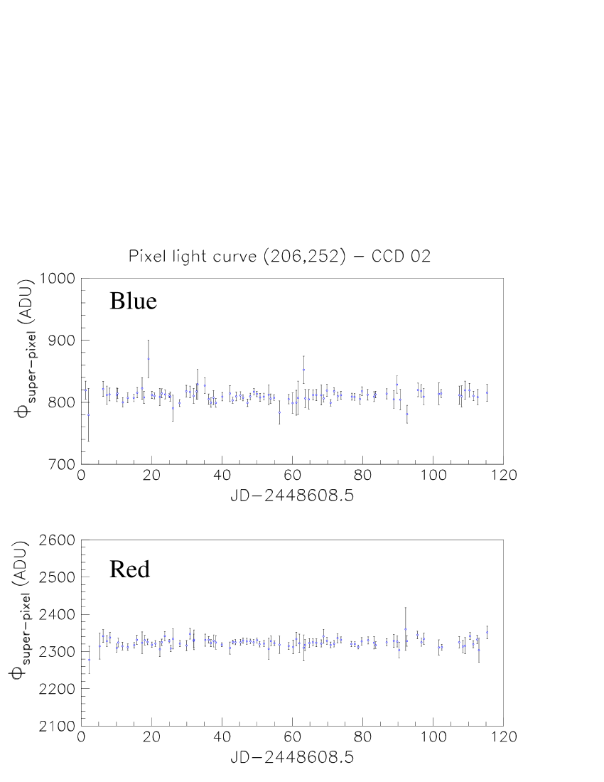
Figure 25: Example of a stable super-pixel light curve.

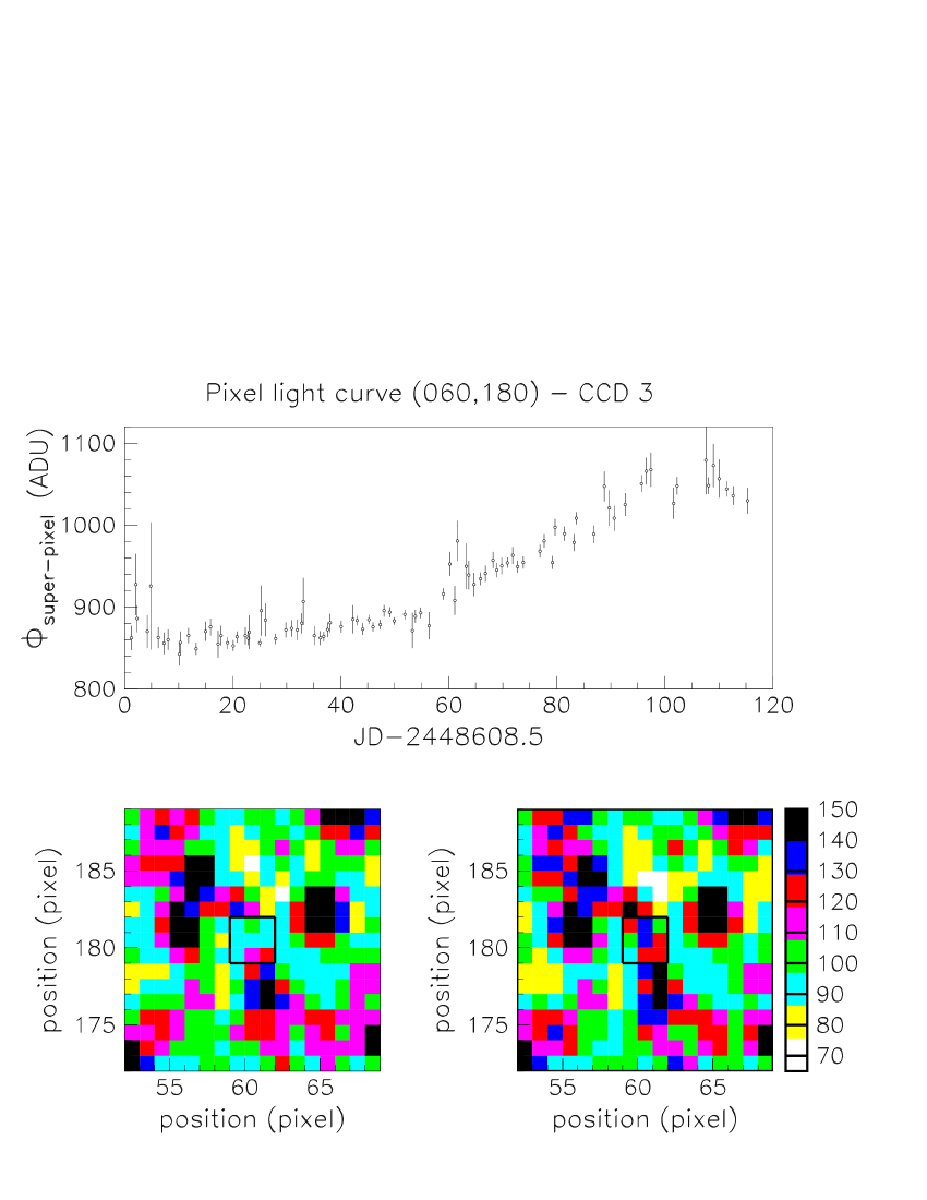
Figure 26: Example of a variable super-pixel light curve in blue (top). The star is unresolved at minimum (bottom left panel) and would even be difficult to detect with classical procedures at maximum (bottom right panel).

We have now super-pixel light curves with an error estimate for each flux. Figure 25 displays an example of a typical stable light curve in blue (upper panel) and in red (lower panel), whereas Fig. 26 is an example of a variable light curve. The error bars obtained as a combination of expected photon noise and experimental data are compatible with the dispersion observed on the super-pixel light curves, and allow us to give a different weight to each measurement according to its quality.

8 Conclusion

The treatment described here has produced $2.1\times 10^{6}$ super-pixel light curves corrected for observational variations, with an error bar for each point. They are characterised by an average stability close to twice the photon noise: dispersions of 1.8% of the flux in blue and 1.3% in red are measured over a 120 days time period. To reduce the effects of the dispersion due to the observational conditions, averaging the images of each night turns out to be a crucial step. The fluctuations due to seeing variations have been corrected for. We associate an error bar with each measurement, and these careful estimates together with the study of possible systematics are used in the companion papers for the detection of intrinsic luminosity variations.

This study is the starting point for the comprehensive microlensing search described in Paper II. The error estimates enter the definition of the selection criteria and constitute an important ingredient for microlensing Monte-Carlo simulations required to quantify the efficiency of the pixel microlensing method. The study of the background of variable stars will be addressed in Paper III.