The Kinematic Composition of Mgii Absorbers

Abstract

The study of galaxy evolution using quasar absorption lines requires an understanding of what components of galaxies and their surroundings are contributing to the absorption in various transitions. This paper considers the kinematic composition of the class of $0.4<z<1.0$ Mgii absorbers, particularly addressing the question of what fraction of this absorption is produced in halos and what fraction arises from galaxy disks. We design models with various fractional contributions from radial infall of halo material and from a rotating thick disk component. We generate synthetic spectra from lines of sight through model galaxies and compare the resulting ensembles of Mgii profiles with the $0.4\leq z\leq 1.0$ sample observed with HIRES/Keck. We apply a battery of statistical tests and find that pure disk and pure halo models can be ruled out, but that various models with rotating disk and infall/halo contributions can produce an ensemble that is nearly consistent with the data. A discrepancy in all models that we considered requires the existence of a kinematic component intermediate between halo and thick disk. The variety of Mgii profiles can be explained by the gas in disks and halos of galaxies not very much different than galaxies in the local Universe.

In any one case there is considerable ambiguity in diagnosing the kinematic composition of an absorber from the low ionization high resolution spectra alone. Future data will allow galaxy morphologies, impact parameters, and orientations, Feii/Mgii of clouds, and the distribution of high ionization gas to be incorporated into the kinematic analysis. Combining all these data will permit a more accurate diagnosis of the physical conditions along the line of sight through the absorbing galaxy.

Accepted for publication: Astrophysical Journal

1 Introduction

Quasar absorption lines (QALs) provide a diagnostic of the gaseous conditions in and around galaxies as they form and evolve. Most Mgii absorbers at $z<1$ are produced within $40h^{-1}$ kpc of known $>0.1L^{*}$ galaxies (Steidel (1995)). High resolution spectroscopy (HIRES/Keck) shows that they have multiple absorbing components (Churchill, Vogt, & Charlton (1998), hereafter CVC98). These components should provide information about how the Mgii gas is distributed spatially and kinematically. More generally, multiple component structure is apparent in various ionization stages of the different chemical elements probed by QALs over the history of the Universe. Before QALs can be fruitfully applied to a detailed study of conditions in galaxies we must resolve many of the remaining ambiguities inherent in their interpretation.

Based upon low resolution spectra, the Mgii absorbers with $W({{\rm Mg}\kern 1.00006pt{\sc ii}})>0.3$ Å have generally been interpreted as material infalling into the halos of the normal $>0.1L^{*}$ galaxies (Steidel (1995); Mo & Miralda–Escudé (1996)). However, most $L^{*}$ galaxies are disk galaxies, and the disks themselves contain the Hi necessary for ionization conditions that allow Mgii to survive. Disks in the local Universe clearly extend well beyond the optical radii (Irwin (1995)), but it is hard to establish directly the Hi distribution at $N({{\rm H}\kern 1.00006pt{\sc i}})<10^{19}$cm^-2. In a few cases, sensitive 21 cm measurements provide maps of galaxy disks down to $N({{\rm H}\kern 1.00006pt{\sc i}})=10^{18}$cm^-2, and in these cases the disks extend to tens of kpc (Corbelli & Salpeter (1993); van Gorkom et al. (1993)). In the M81 group, interactions lead to large $N({{\rm H}\kern 1.00006pt{\sc i}})$ in a flattened distribution well beyond 50 kpc of M81 itself (Yun, Ho, & Lo (1994)), but some relatively isolated dwarfs have been found to be extended also (Hoffman et al. (1993)). As shown in Charlton and Churchill (1996, hereafter CC96), for a disk with larger scale–height outer regions, the random orientation cross–section is competitive with that of spherical halos. In fact, CC96 argue that after possible biases in the available sample of Mgii absorbers are taken into account, models can be designed that are consistent with either a spherical or a thick disk geometry.

Simply because of the cross–section of known Hi disks, galaxy disks must make some contribution to Mgii absorption. Also, some fraction of absorbing galaxies are diskless (ellipticals), so at minimum there must be contribution to the absorption by these two kinematic components. Here we address the question of what the dominant contribution is to Mgii absorption. Is the larger fraction of the Mgii column density from disk material or from halo material? Does the answer to this question vary from galaxy to galaxy or from one line of sight to another within a single galaxy?

Based upon the absorption properties along lines of sight through the Milky Way and through nearby galaxies, we can begin to infer the answers to these questions at $z=0$. Lines of sight looking out from our special vantage point in the Milky Way pass mostly through disk material, and from the ratios of various transitions and their positions in velocity along the line of sight, the nature of the absorbing clouds can be inferred as Hi regions, Hii regions, superbubbles, or high velocity halo clouds (Spitzer & Fitzpatrick (1993); Fitzpatrick & Spitzer (1994); Spitzer & Fitzpatrick (1995); Welty et al. (1997)). As with these many Galactic sight–lines, at higher redshifts there is considerable kinematic variation in the profiles. Churchill, Steidel, and Vogt (1996, hereafter CSV96) show that the variations in the HIRES/Keck profiles of $0.4<z<1.0$ Mgii absorbers are not strongly correlated with the impact parameter, luminosity, or morphological type of the identified absorbing galaxy. The large scatter in the relationships between absorption and galaxy properties could be produced by variations due to clumpiness and discrete structures that lead to variations within the individual galaxies.

The variations due to clumpy structures will complicate efforts to extract kinematic information from individual profiles. Earlier studies of kinematic signatures demonstrated the basic profile shapes expected from various spatial and kinematic laws (Weisheit (1978); Lanzetta & Bowen (1992)). Lanzetta and Bowen suggested that a trend might exist where rotating disk signatures are characteristic of small impact parameter Mgii absorbers, while “double–horned” infall profiles arise in the outer halos of the galaxies. The scatter observed in the relationships between impact parameter and absorption profile properties indicates that the situation is more complicated (CSV96). There is hope that a given population of absorbers will give rise to profiles that reflect the underlying kinematic and spatial distributions in their host galaxies, but it is important to consider the effect of stochastic variations on these profiles. Prochaska and Wolfe (1997) showed synthetic profiles produced by clouds selected from a thick exponential rotating disk and found that this kinematic law is consistent with the properties of high redshift damped Ly$\alpha$ absorbers.

In this paper we compare the properties of an ensembles of profiles drawn from various kinematic models (and combinations of kinematic models) to the ensemble of observed HIRES/Keck profiles of $0.4<z<1.0$ Mgii absorbers. The following four questions motivate our simulations.

1. Is it possible to extract enough information from a particular profile to identify it as associated with a particular kind of galaxy, a line of sight through a particular part of a galaxy, a galaxy undergoing some particular stage of formation or evolution, etc.? To what extent will we be able to resolve the kinematic ambiguities?

2. Can the statistical properties of the observed ensemble be reproduced by a population of disks and/or halos of galaxies? The Mgii absorbing galaxies at $0.4<z<1.0$ cover all morphological types and the range of luminosities down to $0.1L^{*}$. Are there profiles that require unusual kinematic laws or are all of them consistent with what we would expect for lines of sight through the population of galaxies at $z=0$?

3. Can the variety of observed absorption profiles be reproduced within the context of a single kinematic model, or a weighted combination of two (such as disk and halo)? Can variations in the profiles be due to the expected line of sight differences through one class of galaxies or are the profiles too varied?

4. In view of future studies, what role will kinematic analysis of high resolution absorption profiles of low ionization gas play in broader studies that also include galaxy properties, Ly$\alpha$, and higher ionization gas? By combining this information, will we be able to extract information about the conditions along a sight–line through a particular galaxy, and about the global properties of the galaxy at the same level as is done through the Galaxy?

The answers to these questions may lead to a characterization of the population of Mgii absorbers at $0.4<z<1.0$ in terms of their kinematic composition. In this redshift range the absorbing galaxy can more readily be identified and studied, providing more leverage on the interpretation of absorption properties. Lines of sight through N–body hydrodynamic simulation boxes (which also model the ionization states of various metals) show that different kinematic signatures result from galaxies at different stages of evolution (Rauch, Haehnelt, & Steinmetz (1997)). A population of absorbers could be dominated by the kinematics of material that has just separated from the Hubble flow, material falling into a galaxy halo, or material in a well–formed disk. Establishing the contributions of spatial and kinematic components to Mgii profiles at low to intermediate redshift is prerequisite to interpreting their evolution as the redshift range of observability increases through studies in the UV and near–IR (Churchill 1997b ).

The second section of this paper presents the 26 observed $0.4<z<1.0$ Mgii profiles and discusses the selection and analysis of this sample. Even a qualitative examination of these profiles suggests certain interpretations of their kinematic composition. Guided by these interpretations and by properties of nearby galaxies we designed kinematic models. The details of the model construction are outlined in §3, which also describes our statistical comparisons of the observed and model spectra. The results of our analysis is given in §4, where we address which of the kinematic models are formally consistent or inconsistent with the ensemble of observed spectra. In §5, we return to the four questions posed in this introduction and assess the extent to which we can characterize the kinematic and spatial distribution of the population of $0.4<z<1$ Mgii absorbers.

2 HIRES/Keck Observations of $0.4<z<1.0$ Mgii Absorbers

The observed sample for comparison to kinematic models has been selected from the larger study of Mgii absorbers with equivalent width $W(2796)>0.3$Å (Churchill 1997a ; CVC98). Although the full data set included systems out to $z=1.8$, for two reasons we choose to limit this study to the $z<1$ Mgii absorbers. First, this sample is unbiased in equivalent width below this redshift cutoff, while several of the higher redshift systems were selected to be particularly strong. More importantly, there could be an evolution in the kinematic properties of the global population of galaxies over the larger redshift interval $0.4<z<1.8$. The redshift interval of $0.4<z<1.0$ covers the lookback time $\sim 4-9$ Gyr.

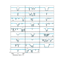
Figure 1: The observed Mgii(2796) profile for $0.4<z<1.0$ systems. The 5$\sigma$ rest–frame equivalent width limits range from 0.007 Å up to the cutoff of 0.02 Å. The Voigt profile fits are drawn as a narrow line superimposed on the data, and the ticks mark the locations of the centers of the profiles in velocity space. For those few systems with $v>\pm 260$ km s^-1 clouds, the vertical dotted lines mark the optical depth weighted mean, which defines $v=0$ km s^-1.

The data were obtained with the HIRES spectrometer (Vogt (1994)) on the Keck I telescope and have a spectral resolution of 45,000, corresponding to 6.6 km s^-1 (Churchill 1997a ; CVC98). In addition to the Mgii $\lambda\lambda 2976,2803$ doublet, Mgi(2853) and several Feii transitions were observed. These prove to be important for the study since they allow more accurate Voigt profile fitting, with a more realistic number of subcomponents in cases where the Mgii doublet is saturated. So that we have a more uniform sample for the kinematic study we also eliminate all systems for which the $5\sigma$ equivalent width detection limit for Mgii(2796) is greater than 0.02Å in the rest frame. In Figure 1, we display only the Mgii(2796) transition for each of the 26 systems, with Voigt profile fits determined using all available Feii, Mgi, and Mgii transitions.

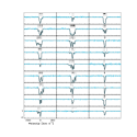
Figure 4: Twenty seven representative profiles from a pure disk model (Pure Disk 2 in Table 1) on the same scale as the data in Figure 1. The upper set of ticks represent the velocities at which clouds in the model were intercepted by the random line of sight. The lower set are the output components obtained from Voigt profile model. More than half of the input clouds are lost to blending in the disk model, and clearly the Doppler parameter distribution broadens as a result.

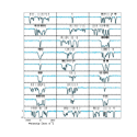
Figure 5: Same as Figure 4, but for the the infall model (Pure Infall 1). Not as large a fraction of components are lost to blending as in the pure disk models.

What follows in this paper is a quantitative comparison of the data to synthetic spectra from the kinematic models. However, visual inspection of the HIRES/Keck Mgii profiles in Figure 1 already leads us to two simple conclusions about the kinematics of these objects. First, many systems are dominated by a strong blended component with a width of 40–100 km s^-1. This range is not consistent with the velocity spread that we would expect for halo kinematics, whether it be infall, outflow, or random isotropic motion (for an example of profiles from infall halo kinematics see Figure 5). Second, in some profiles there are outlying weaker components spread over a larger $\Delta v$ of hundreds of km s^-1. These large spreads are clearly inconsistent with the kinematics expected for a rotating disk, even when random vertical motions are included (see Figure 4 for examples of disk kinematics). Thus, simply based upon qualitative arguments, it is immediately apparent that some combination of disk and halo kinematics is needed to produce the observed ensemble of profiles. This could require either some galaxies that are pure disk galaxies and others that are pure halo galaxies, or it could imply that some profiles require both a disk and a halo component in the responsible galaxy.

3 The Models and Their Simulated Spectra

We consider models with rotating disk components and with radial infall/halo components. The model disks are extended– we assume a radius of $1.5R(L^{*}_{K})$ where $R(L^{*}_{K})=35(L/L^{*}_{K})^{0.15}$ kpc in order that the population of inclined disks can be consistent with the frequency with which galaxies within $R(L^{*}_{K})$ of quasar lines of sight produce absorption (CC96). Halos are assigned a radius of $R(L^{*}_{K})$. There are five “populations” of kinematic/geometric models that we present in this study: 1) a single population of pure disk models; 2) a single population of pure halo models; 3) a “two–population” model, in which 50% of galaxies are pure disks and 50% are pure halos; 4) a single population of “hybrid” models, in which every galaxy has 75% of its gaseous clouds in a disk and 25% of its clouds in a halo (75D/25H); and 5) a single population of “hybrid” models, in which every galaxy has 50% of its clouds in a disk and 50% of its clouds in a halo (50D/50H).

In the course of our study, we investigated two–population models with various fractions of disk/halo galaxies, but we present only the 50D/50H case for purposes of illustration. We also investigated other hybrid models, each with a different fraction of disk/halo clouds. Again, we show only two of these cases in this paper, but draw upon the general study for our conclusions.

The full problem of the physical conditions of the clouds is presently intractable. Our goal is simply to test the kinematic distribution of absorbing clouds and to rule out certain classes of models, if possible (we make no attempt to diagnose the cloud chemical abundances or photoionization properties). Thus the individual cloud properties are selected from the measured distributions of column densities and Doppler parameters (Churchill 1997a ; CVC98). More precisely, we draw from underlying distributions that produce profiles consistent with the observed distributions once the simulated spectra are analyzed in the exact same way as were the data.

The basic simulation procedure is as follows. For each simulated line of sight we pick a galaxy from the Schechter luminosity function with $\alpha=-1$. Its rotation or radial infall velocity is given by the Tully–Fisher relation. Spherical clouds are placed in a spatial distribution and each of these clouds is assigned a velocity based upon a simple kinematic. Each cloud is assigned a Mgii column density selected from a power law distribution and a Doppler parameter selected from a Gaussian with a low–end cutoff. The “best” power law exponent and Doppler parameter spread and cutoff depends upon the amount of blending in a particular model. Once the model galaxy is defined, we run a line of sight through it at impact parameter chosen by area weighting considerations and determine which clouds are intercepted. Using the velocities, column densities, and Doppler parameters of these clouds, we generate simulated spectra. These spectra are then convolved with the HIRES instrumental profile, sampled with the pixelization of the HIRES CCD, and degraded to have signal to noise $S/N$ ratios consistent with the data. The $S/N$ of any given simulated spectrum is chosen from the $S/N$ distribution of the data. We generate the Feii profiles also, assuming thermal scaling of the Doppler parameters, and applying the observed relation

$$\log N({{\rm Fe}\kern 1.00006pt{\sc ii}})\simeq\log N({{\rm Mg}\kern 1.00006pt{\sc ii}})-0.3,$$ (1)

for the column densities. Thermal scaling is consistent with the observed ratios of the Mgii and Feii Doppler parameters (Churchill 1997a ; CVC98). Having followed this procedure we have a set of spectra very similar to the observations and we can proceed to analyze them in precisely the same manner.

The profile fitting procedure used in our analysis is a two step process. The first step is an application of the automated Voigt profile fitter, autofit (Davé et al. (1997)), which we have modified to account for broadening due to the instrumental spread function. autofit was applied to the Mgii(2796) transition and this solution was scaled to give parameters for the Voigt profiles to model the Mgii(2803) and Feii transitions. This initial model was refined using minfit (Churchill 1997a ), a maximum likelihood least–squares fitter. MINFIT minimizes the $\chi^{2}$ between the data and the Voigt profile model by adjusting the column densities, Doppler parameters, and number of Voigt profile components (with the goal of minimizing the number of these components).

3.1 Detailed Procedure

For infall/halo models we place the clouds randomly within the spherical distribution of radius $R(L_{K})$. The magnitude of each cloud velocity is set equal to the value given by the Tully–Fisher relation and its direction is radial towards the center of the sphere. In practice, each cloud is taken to have a radius of 1 kpc, but this is rather arbitrary since a cloud radius which is smaller would then require a larger number of clouds per halo such that the number of intercepted clouds remains conserved at a number consistent with the data. Thus we describe each model by its integrated cross sectional area, $N\sigma_{\rm cl}$, equal to the number of clouds times the cross section of each.

For disk models there are a larger number of parameters and assumptions. The disk is taken to have a full height of 1 kpc out to a radius of 10 kpc, increasing linearly to a 10 kpc height at its maximum radius of $1.5R(L_{K})$. The clouds are rotating differentially with a flat rotation curve with velocity given by the Tully–Fisher law. In addition each cloud is assigned a velocity in the direction perpendicular to the disk, selected from a Gaussian distribution with $\sigma=15$ or $25$ km s^-1.

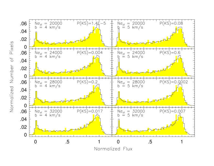
Figure 2: Distributions of the number of pixels, in the region of a detected Mgii feature, with a given flux value. This is a portion of the grid of 36 models explored for a 50D/50H hybrid model. The data are depicted by the shaded region, and the models by the solid histogram. Each panel is labelled with the cloud cross section, $N\sigma_{\rm cl}$, and the mean Doppler parameter of the Gaussian distribution, $b$. Also shown are the Kolmogornov–Smirnov test probability that the model fluxes were selected from the same distribution as the data. For all models, the disk component has a vertical velocity dispersion $V_{z}=25~{}{\hbox{km~{}s${}^{-1}$}}$ and the power–law slope of the input column density distribution is 1.74. Models with $b=4(5)~{}{\hbox{km~{}s${}^{-1}$}}$ have a $\sigma(b)=2(3)~{}{\hbox{km~{}s${}^{-1}$}}$ and a lower cutoff of 2 km s^-1. In each vertical sequence of 4 panels, the gradual increase in the number of saturated pixels can be recognized as a consequence of the increasing number of clouds.

For a given kinematic model we must find the location in the parameter space of cloud property distributions that results in spectra that are consistent with the observed column density and Doppler parameter distributions. The parameters that describe the input cloud distributions are the slope of the Mgii column density distribution, and the Gaussian $\sigma$ and lower cutoff of the Doppler parameter distribution. The column density distribution has a lower cutoff of $\log N({{\rm Mg}\kern 1.00006pt{\sc ii}})=11.3$ cm^-2 for all grid points. This is the minimum cloud that could be detected for the highest $S/N$ spectrum in our sample. It is not practical to fit all profiles for each grid point, thus we have devised a test that relies on the flux distribution of all pixels within absorption features. In Figure 2, this test is illustrated for a small region of one of our model grids, which includes the cloud properties and the number of clouds in the galaxy as parameters. In fact, because of the large number of pixels in the distributions, this test provides a sensitive method for refining the grid. In order to find a compatible model, it was critically important to give the model spectra the same distribution of $S/N$ as the data. From a typical grid of 24–48 choices of parameters (for a given kinematic model) we considered only models that showed a probability of more than 1% by the Kolmogornov–Smirnov test to be drawn from the same pixel flux distributions as the data. Typically, this techniques allowed us to exclude all but 3–5 grid points, which we then profile fit and conducted further statistical comparisons.

In Table 1, we list the parameter choices that yielded adequate fits for various classes of models, along with their KS probabilities. Typically, the effect of blending can be compensated by a steeper power law for the $N({{\rm Mg}\kern 1.00006pt{\sc ii}})$ distributions, since the lowest flux pixels are often the result of the combined effects of several lines. Increasing the vertical velocity dispersion of the disk kinematics decreases the number of saturated pixels. An increase in $N\sigma_{\rm cl}$ can be compensated by a decrease in the mean Doppler parameter, but ultimately the output Doppler parameter distribution from fitting must match the observed Doppler parameter distribution.

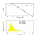
Figure 3: This figure gives the results for 100 realizations of a 50D/50H hybrid model. (upper panel)— The model column density distribution output, after Voigt profile fitting. The model distribution compares well with that of the data, which were also fit by a power law with slope 1.74 (dotted line) down to approximately $\log N({{\rm Mg}\kern 1.00006pt{\sc ii}})=12.3$. Except for disk models with small vertical velocity dispersions, $V_{z}$, the slope of the column density distribution is not heavily affected by blending. However, the lower cutoff is sensitive to the disk velocity dispersion. (lower panel)— The input Doppler parameter distribution (dotted) is dramatically affected by blending, resulting in a broader output distribution with a larger mode. A KS test shows that the output distribution (solid) is not inconsistent with that of the data (shaded).

From a maximum likelihood fit to the observed distribution of $0.4\leq z\leq 1.0$ Mgii absorber column densities, we obtain power–law slope of $\delta=1.74$ to $n(N)\sim N^{-\delta}$ with lower cutoff $\log N=12.5$ cm^-2. In fact, for models with flux distributions consistent with the data, we found that the slope of the output column density distribution was similar to the input slope, over a reasonable fitting range. Therefore an input slope of $\delta=1.74$ was suitable. The Doppler parameter distribution of observed data, excluding values with fractional errors greater than unity, is best fit by a Gaussian truncated at 2–3 km s^-1, with a peak of 3.5 km s^-1 and a standard deviation of 3–4 km s^-1. An input Doppler parameter distribution with a mean of 3–4 km s^-1, a $\sigma$ of 2 km s^-1, and a lower cutoff of 2 km s^-1 led to a good fit of the output distribution with the observed data. The output distributions of column densities and Doppler parameters for a consistent hybrid model with 50D/50H contributions are compared to the input and observed data distributions in Figure 3. Based on these considerations we select the following models listed in Table 1 for further analysis: Pure Disk 2, 75D/25H Hybrid 2, 50D/50H Hybrid 2, Pure Infall 1, and a two–population mix in which half the systems are Pure Infall 1 and half are Pure Disk 2

3.2 Statistical Analysis

Statistical tests fall into three categories:

(1) Pixel by pixel comparisons: These tests involve the distribution of the number of pixels or pixel pairs satisfying various criteria. These have the advantage of large number statistics so that F–tests and KS tests are very sensitive to differences in model distributions. This is why the pixel flux distribution was judged an effective method to refine the model grid in the previous section. The disadvantage of these types of tests is that they average together the differences between individual systems, and thus they do not test whether a model can explain the variation in properties from system to system.

(2) System by system statistics: The test compare the profile shape and the Voigt profile model cloud properties system by system. Examples of these statistics are the various moments of the profiles of entire systems (weighted by the apparent optical depth) and the number of clouds per system. These test are subject to small number statistics; comparisons can only be so good as the statistics on the 26 profiles in the observed sample permit.

(3) Cloud or subfeature statistics: These tests are in some ways intermediate between the previous two. A subfeature is defined as a detected region of a spectrum that is separated from other detected pixels by at least 2.5 HIRES resolution elements. An example of a subfeature statistic is the number of subfeatures in a given velocity bin. Cloud properties are parameterized by the Voigt profile fit column densities and Doppler parameters. An example of a cloud statistic is the cloud–cloud two point clustering function. These statistics combine the individual systems and thus average out variations between them like (1). Although they are subject to small number statistics, there are more subfeatures and clouds than there are systems, so they are somewhat better in that sense than (2).

Many plethora of these tests were performed on all models and on the data. For presentation we choose a range of tests that best distinguish the various differences that could exist between our models. The following battery was selected: (A) $\Delta V$ of pixel pairs for which both pixels fall in the same flux bin 0.0–0.2, 0.2–0.4, 0.4–0.6, 0.6–0.8, and 0.8–1.0; (B) Histogram of number of clouds per system; (C) Histogram of optical depth weighted velocity widths, $\omega_{v}$, for systems, where

$$\omega_{v}^{2}=\int_{v_{1}}^{v_{2}}\tau_{a}(v)\left(v-\left<v\right>\right)^{2}dv/\int_{v_{1}}^{v_{2}}\tau_{a}(v)dv,$$ (2)

and $\tau_{a}$ is the apparent optical depth defined by

$$\tau_{a}(\lambda)=\ln\left[{I_{c}(\lambda)}\over{I(\lambda)}\right].$$ (3)

The zero point of velocity $\left<v\right>$ is defined such that half of the integrated apparent optical depth lies blueward and half lies redward of that point; (D) Histogram of equivalent width for systems; (E) Histogram of number of subfeatures as a function of velocity; (F) Two Point Clustering Function, defined as the distribution of velocity differences for all cloud pairs within single systems, taken for the full sample of systems. The cloud velocities are taken from the Voigt profile fits.

Our formal statistical comparisons between the models and the data used the KS test and the F–test. Neither test is ideal for comparing distributions with arbitrary shape. The KS test is not sensitive to the tails of the distribution. The F–test compares the variance of the distribution, but is not sensitive to its precise shape. In order to claim a model is inconsistent with an observed distribution it is sufficient that only one of the two tests gives a small probability that the observed and model distributions are drawn from the same parent distribution. It is important to appreciate that if both tests give a relatively large probability, this does not prove consistency.

Before beginning to discuss the result of these statistical comparisons for the various models, an important caveat should be discussed. Double galaxies (i.e. close galaxy pairs) are not treated in our kinematic models, but some almost certainly do exist in the observed sample. The presence of double galaxies can change the statistics considerably, leading to a much larger number of large velocity clouds and subfeatures. Thus we must be cautious in our interpretations not to hastily rule out a model because it underpredicts high velocity components.

The make a more quantitative assessment of the double galaxy issue we consider a second sample (S2) of the observed 26 systems in which we eliminated from consideration three systems with total velocity spreads greater than 350 km s^-1. Those profiles that have been excluded from Sample S2 are marked with a “$\ast$” in Figure 1. It is impossible to unambiguously separate double galaxies and satellite galaxies from the observed sample, but we have adopted this fairly extreme approach. We also separate a fourth system (marked with a “$\ast\ast$” in Figure 1) into two systems and include these two instead in Sample S2. The split is made in between the two separate components that are observed in Civ $\lambda\lambda 1548,1550$ of the FOS/HST spectrum (Churchill 1997b ; Churchill et al. (1997)). Sample S2 has 24 systems. We analyzed both the full sample (S1) and Sample S2, and we discuss both in the following section.

4 Results of Kinematic Models

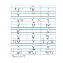
Figure 6: Same as Figure 4, but for the hybrid model (75D/25H Hybrid 2). The “long” ticks in the upper set mark the input halo clouds and the “short ticks” mark the input disk clouds. In these hybrid models, the line of sight often intercepts only disk clouds, though sometimes only halo clouds are intercepted. Outlying components in velocity space (from the disk kinematic center) are sometimes produced by an occasional halo cloud and this brings the model into better agreement with the data than a pure disk model.

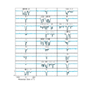
Figure 7: Same as Figure 4, but for the hybrid model (50D/50H Hybrid 2). The “long” ticks in the upper set mark the input halo clouds and the “short ticks” mark the disk clouds. This high halo to disk fraction results in a larger kinematic spread than seen for the 75D/25H models (see Figure 6).

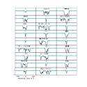
Figure 8: Same as Figure 4, but for the two–population model (50% Pure Disk 1 and 50% Pure Halo 2). This figure allows one to speculate as to which of the profiles represent disk kinematics and which represent halo kinematics. The panels with “long” ticks in the upper set are from pure halo models and those with “short” ticks are from pure disk models. In about 1/3 of the cases, the ambiguity is severe and one cannot make an educated guess as to the component of origin of the profile.

Sample profiles of the models of various types, selected from the grid in Table 1, are presented in Figures 4–8. These models are most consistent with the pixel flux distribution as well as with the observed column density and Doppler parameter distributions. Illustrated are 27 profiles each for: the Pure Disk models (Figure 4); the Pure Infall models (Figure 5); the 75D/25H Hybrid models (Figure 6); the 50D/50H Hybrid models (Figure 7); and, the 50/50 two–population models (Figure 8). The 50/50 two–population models shown in Figure 8 are drawn from the models presented in Figures 4 and 5. This population illustrates the ambiguity that could exist in classifying any given observed system.

4.1 Pixel by Pixel Statistics

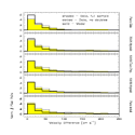
Figure 9: The distribution of velocity differences between all pairs of pixels with flux values $<0.2$ in detected features. The shaded histogram is the distribution for the data (Sample S1). The dotted histogram is for Sample 2, and illustrates how this distribution is changed when we attempt to remove all double galaxies. The solid curves in the five panels are model results, with increasing infall/halo content from top to bottom. The 50D/50H hybrid model produces a similar distribution overall as the two–population mix of pure disk and pure halo models. The single population pure disk and pure halo models are very inconsistent with the data over the full velocity range. All models are inconsistent with the data in the range 20–80 km s^-1, which demonstrates the need for a kinematic component intermediate between halo and disk.

We adapted a procedure developed in Cen et al.(1997) and considered the pairwise velocity differences for pixels in various flux bins and within a system. We also examined the distributions of velocity relative to the velocity zero point determined by the apparent optical depth, as described in §3. Since the zero point of the system does not necessarily bear any relationship to a real kinematic component, we opt to present pixel velocity differences since they are independent of these considerations. In Figure 9, we show the distribution of velocity differences for all pixel pairs in which both pixels have a flux between 0.0 and 0.2, i.e. for the saturated pixels. In each panel, the model histogram is compared to both observed samples S1 and S2 (the full sample and one with possible double galaxies removed). The pure disk model distribution is quite narrow compared to the data, and the pure infall model is too broad. This is consistent with the visual impression from Figures 4–8. As more disk component is added to a model the distribution gets narrower and the tail is reduced. Two–population models naturally have both the narrow distribution and the large tail at high velocity differences.

For the 0.0 to 0.2 flux bin, none of the models is in agreement with the Sample S1 data according to a KS test. There are two reasons for this. First, the pixel by pixel statistics are quite sensitive tests. It is very difficult to tune the parameters so that the distributions agree to the level where the KS test will not distinguish significant differences. Second, there is a systematic difference between these models and the data which no amount of fine tuning can alleviate. The difference is a deficit of saturated pixel pairs in the bins with velocity difference 20–80 km s^-1. The vertical velocity dispersion for the disk components in displayed models was $V_{z}=25$ km s^-1. Increasing this value would reduce the inconsistency between the models and the data, however it would have to be increased substantially to bring them into agreement. At that point we would have a kinematic component that did not bear much resemblence to a thick disk. We conclude that there is a kinematic component contributing to the observed absorbers that is distinct from a thick disk or a infall/halo component.

We also considered the velocity difference distributions for pixels with flux ranges 0.2–0.4, 0.4–0.6, and 0.6–0.8. The same discrepancy present in the 0.0–0.2 bin persists in the 0.2–0.4 bin, however it gradually becomes less extreme. Pure infall and pure disk models predict highly discrepant distributions for the 0.4–0.6 and 0.6–0.8 flux pixels, but the hybrid 50D/50H and the two–population 50% pure disk and 50% pure halo models, with $V_{z}=25$ km s^-1, are reasonably consistent A disk vertical velocity dispersion of 15 km s^-1 produces distributions that are too narrow.

Finally, we consider the effect that double galaxies, that may exist in the observed sample, would have on these conclusions. For this purpose, we also analyzed Sample S2, described at the end of §3. The dotted histogram presented in Figure 9 represents the distribution of velocity differences for saturated pixels for Sample S2. Note that compared to Sample S1, the S2 distribution becomes somewhat narrower and the large velocity difference tail is reduced. From this we see that conclusions about specifically which models provide the best fit are quite sensitive to whether certain particular observed systems are included in the sample. However, the large discrepancy between all models and the data in the 20–80 km s^-1 bins is pronounced regardless of whether Sample S1 or S2 is used.

4.2 System By System Statistics

4.2.1 Number of Clouds Per System

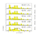
Figure 10: The distribution of the number of clouds per system, $N_{\rm cl}$, from the Voigt profile fits. The shaded histogram is the distribution for Sample S1 of the data. The dotted histogram is for Sample S2. As models become less blended the number of clouds obtained from the fit increases. Noted on each panel are the KS and F–test results for comparison of the model to Samples S1 and S2. Given the small number statistics, only the pure disk model can be definitively ruled out by these tests, although the pure infall model also has low probabilities.

As expected, the number of clouds found by the automated profile fitting procedure decreases as the disk contribution increases, due to blending. This is illustrated in Figure 10, along with the observed distribution of the number of clouds per system for Samples S1 and S2. The pure disk model is clearly discrepant with both observational samples, with the KS test yielding a probability less than $7\times 10^{-8}$ and $8\times 10^{-6}$ that the model and observational distributions were drawn from the same distribution. The hybrid model with 75D/25H contributions does not produce the outlying points at large $N_{\rm cl}$ in Sample S1, but is consistent with Sample S2. The pure infall model is inconsistent with the $N_{\rm cl}$ distribution in Sample S1, and is only marginally consistest by both the KS and F–tests once the double galaxy systems are removed in Sample S2. The two models (hybrid and two–population) with 50/50 contributions fare best by the combination of tests, each having greater than 3% chance of being drawn from the same distribution as the data for either sample.

4.2.2 Velocity Widths

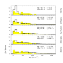
Figure 11: The velocity width distribution for systems from selected models compared with Samples S1 (shaded) and S2 (dotted). The velocity width distribution depends strongly on the model. Any of the three models with both disk and halo kinematics is consistent with the observed profiles for Sample S1. All models (except pure disk) produce an excess of large velocity widths as compared to Sample S2, in which an extreme criterion was applied for double galaxy removal.

In Figure 11, the distribution of system velocity widths for various models is compared to the two observed samples. The more consistent models, with Sample S1, have between a 50% and a 75% disk contribution. In all models but the pure disk the high velocity tail is too large relative to Sample S2. However, models could be found that would be consistent with a sample intermediate between S1 and S2. Pure infall models, especially, have too large a tail and this discrepancy becomes larger if we remove the possible double galaxy contribution to the data.

4.3 Cloud and Subsystem Statistics

4.3.1 Subfeature Velocity Distribution

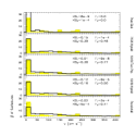
Figure 12: The velocity distribution for subfeatures in the five selected models, compared to the two observed samples, Sample S1 (shaded) and Sample S2 (dotted). A subfeature is defined as a distinct detected region, and the velocity of a subfeature is measured relative to the zero point of the system, defined as the mean of the profile weighted optical depth. The tail is much larger for models with significant halo contribution. Determining which model is most consistent with the data is dependent upon which of the observed samples (with or without suspected double galaxies) is being compared.

The distributions of central velocities for subfeatures (detections separated in velocity space by 2.5 HIRES resolution elements or 7 pixels) are presented in Figure 12. Again, the zero point velocity is defined by the apparent optical depth technique. Pure infall models produce much too large a fraction of subfeatures at $v>20$ km s^-1, while pure disk models produce too few. The F–test is especially sensitive to the $>300$ km s^-1 observed data points and thus shows inconsistency between all models and Sample S1. All three intermediate models could be consistent with Sample S2, however. The preferred model depends upon which observational sample is being compared. Thus, it is not feasible to finely distinguish between the models using this test, which is strongly dependent on the high velocity tail.

4.3.2 Two Point Clustering Function

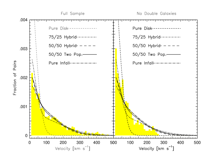
Figure 13: The two point clustering function (TPCF) for the five selected models, compared to Sample S1 (left panel) and to Sample S2 (right panel). The two observed samples differ dramatically, indicating that kinematic indicators are often sensitive to a few systems in a small observational sample. In either case, at least two kinematic components seem necessary to fit the observed distribution. The vertical velocity dispersion of the disk component, $V_{z}$, can be tuned to match the smaller velocity spread component of the TPCF.

The two point clustering function (TPCF) for various models is illustrated in Figure 13 by the double Gaussian fits to the model distibutions. There is a systematic shift toward a narrower TPCF as the fraction of disk contribution is increased. This is to be compared to the two histograms for the observed Samples S1 and S2. For the Full Sample, S1, the best match is to the two–population 50% pure disk/ 50% pure infall model. The pure disk and 75D/25H hybrid models are too centrally peaked, while in the 60–140 km s^-1 range, the pure halo and the 50D/50H hybrid models overproduce pairs of clouds as compared to the number observed. The two–population model combines the appropriate narrow and broad components, where the narrow component can be well tuned by adjusting the disk $V_{z}$. All models but the pure disk produce too large a tail in the TPCF compared with Sample S2, but this is very sensitive to just how we define the observed sample. It appears that a large disk contribution is needed for consistency with this sample.

4.4 Discussion of Results

Many more statistical descriptions of the profiles have been considered than were presented above, but the basic points were illustrated. Although some classes of models can be ruled out, it is in fact quite difficult to quantify the differences between ensembles of profiles. A lot of the difference between the models appears as the system by system characteristics, i.e. we would like to know whether a given observed system could be consistent with being drawn from a distribution of systems produced by a given model. With the pixel by pixel statistics the discriminatory power is very good, so much so that we found a fundamental difference between all the models and the observed profiles. However, even with these tests the information is being considerably diluted by averaging all of the systems together rather than looking at them one by one. The system by system properties are, as we expected, subject to small number statistics. Diluting the rich absorption profile information into a few or even a single number removes much of the diagnostic leverage available through direct comparisons of model and observed spectra.

With larger observational samples it may be possible to do somewhat better in refining a kinematic model grid. However, it is more important to note that there is no reason at all to expect either that all galaxies are the same or that most galaxies have either pure halo or pure disk contributions to Mgii absorption. The models explored here are idealized but they do provide fundamental information about the kinematic composition of the Mgii systems. We see that both disk–like and halo–like kinematics must contribute to the profiles, and even that an intermediate kinematic component appears necessary. Roughly equal contributions from halo and disk seem consistent with the data, but realistically some galaxies, types of galaxies, or evolutionary stages of galaxies will tend to systematically have more Mgii gas in one component than in the other.

5 Summary and Conclusion

By way of summary, we address the questions raised in §1 of this paper:

It is only possible to extract information about the kinematic composition of individual galaxies in a statistical sense. Some infall/halo models (see Figure 5) could be mistaken for pure disk models (see Figure 4) if they happen to have few outlying clouds. To consider this issue further, a visual inspection of Figure 8, in which half of the profiles are from pure disk and half are from pure halo models, is instructive. In the context of a particular model we can state a probability that a given cloud arises in a halo or a disk. In the hybrid disk/halo models shown in Figures 6 and 7, we can identify the actual location of origin for each “cloud” (as defined by the Voigt profile models). This can then be translated to a probability giving the percentage of the Mgii column density in a system arises from disk material or from halo material. In Figure 14, we present the distribution of fraction of disk contribution for lines of sight through the 50D/50H and through the 75D/25H hybrid models. Even though the majority of the Mgii absorbing material may be in the disk, there is a non–negligible probability that most of the absorption in a given system comes from only the halo. In some cases we could guess successfully where the absorption arises from the kinematic signature in the profiles, but in other cases there are ambiguities that cannot be resolved.

Pure disks absorption or pure halo absorption will not produce sufficient variety compared to the ensemble of observed profiles. However, some individual observed profiles are consistent with being drawn from one or the other pure kinematic component. Basically, as could be seen from the qualitative discussion of the observed profiles in §2, the disk models have too few outlying components to be consistent with the data. The halo models are generally too broad kinematically to be consistent with the fraction of observed profiles that have spreads of less than 100 km s^-1.

Two different classes of models come close to producing profiles similar to those observed. Which model is most consistent depends on what the contribution is to the observed profiles by double galaxies, which are not considered in our kinematic models. In both cases, the relatively strong, blended components are produced by disks and the outlying ones by halos. In fact, the two–population models with 50% pure disk and 50% pure halo model galaxies do produce distributions of pixel velocity versus flux that are fairly consistent with the data, when averaged over all systems in the model ensemble. Although one might expect that the system to system properties would not match, they are consistent statistically due to the small number of observed systems. The other type of models that produce fair agreement with the data are the 50D/50H and the 75D/25H hybrid models. A larger halo component is needed to produce reasonable agreement with the full observed sample than if suspected double galaxies are removed.

In all of the models that we have designed there is consistently one type of disagreement with the observations. As illustrated in Figure 9, the relatively saturated pixels (with fluxes less than 0.4) are seldom at velocity differences 20–80 km s^-1 from the profile center as defined by the apparent optical depth. We conclude that the Mgii absorbers have a kinematic component separate from a halo or thick, rotating disk. This separate component must have a characteristic velocity spread intermediate between halo and disk. A consistent picture would be one where infalling material is gradually decelerating and joining the rotation of the disk (Benjamin & Danly (1997)).

5.1 Prospects for Distinguishing Kinematic Components

This paper has been limited to the interpretation of kinematics of high resolution spectra of low ionization gas. With only this information, it is clear that ambiguities remain in determining which kinematic components are responsible for absorption, and thus in making global interpretations about galaxy evolution. However, there is considerably more information that is or will soon be available about the properties of the absorbing galaxies and their gas. We conclude by discussing the prospects for studying galaxy formation and evolution incorporating this additional information.

It is common for the ratio of Feii to Mgii to vary significantly (by more than an order of magnitude) in velocity space across a system. There are two likely causes of this variation: the differing dust depletion for iron and magnesium, and the relative contributions of Type Ia versus Type II supernovae (SNe) to the chemical enrichment local to the galaxy. In the Galactic ISM, iron is depleted by almost one order of magnitude more than magnesium (Lauroesch et al. (1996)). The relative iron depletion is not as severe in the halo (Savage & Sembach (1996)), meaning that for a given abundance pattern, the gas–phase iron to magnesium ratio would be higher in the halo than in the disk. Type II SNe produce $\alpha$–elements, such as magnesium, over short time scales, whereas Type Ia SNe are high iron producers over a longer timescale. The abundance patterns of Galactic halo and old disk stars are seen to have enhanced $\alpha$–elements and $[\hbox{Fe/H}]<-1$ (Lauroesch et al. (1996)), suggesting that in earlier times these stars formed before Type Ia SNe had significantly influenced the chemical content of our Galaxy. The two effects (dust depletion and stellar evolution) work in opposite directions in their effects on the iron to magnesium gas–phase abundance ratio, but generally the net result is that iron is enhanced in disk material. If the gas in halos is continuually recycled, then the iron to magnesium abundance ratio should increase with decreasing redshift as the Type Ia iron enrichment is cycled into the halo from the disk. Interestingly, Srianand (1996) found that the equivalent width ratio of Feii(2382) to Mgii(2796) follows this trend, based upon the low resolution sample of Steidel & Sargent (1992). The wild card here, however, is that the UV ionizing spectrum and possible mechanical ionization sources could be very different in the disk relative to the halo. Since ionization corrections are required to infer the abundance pattern, attempts to exploit this approach will likely be plagued by uncertainties. Similar considerations might allow us to argue whether absorption arises through material in a dwarf satellite galaxy as opposed to halo material. These considerations lead us to suggest that there may promise to resolve the ambiguity between halo and disk absorption components of galaxies and to address the level of halo/dnisk interaction in absorbing galaxies.

It has already been demonstrated that there is a large amount of scatter in any relationships that might exist between galaxy impact parameter, luminosity, or color and Mgii absorption properties (CSV96). Within the context of any given model, we can determine how strong these relationships should be. The mean velocity deviation of a subcomponent cloud from the median velocity, $A(\Delta V)$, provides a good measure of the velocity spread of the system. In Figure 15, we show several models scatter diagrams of $A(\Delta V)$ of each system versus the impact parameter of the absorbing galaxy. Note the trend for the disk components to have smaller numbers of clouds and smaller velocity spreads. Pure infall models do not have many points in the region of the diagram at small impact parameter and small $A(\Delta V)$. While two–population models can fill in this empty region, hybrid models cannot because the halo clouds in each galaxy combine with the disk clouds to create a larger $A(\Delta V)$. Identification of the absorbing galaxies for a larger sample of Mgii absorbers should allow us to distinguish between two–population and hybrid disk/halo models. More simply stated, it will be possible to determine whether or not it is common for disk galaxies to have little Mgii absorbing material in their halos at small impact parameter.

The distribution of the high ionization gas associated with the population of $0.4<z<1$ Mgii absorbers should also be incorporated into an overall kinematic analysis of these systems. The high and low ionization gas are quite possibly distributed in distinct kinematic structures or in different phases of a multi–phase medium (Giroux, Sutherland, & Shull (1994)). There is a large variety in the relationship between high and low ionization gas in the population of $z>2.5$ damped Ly$\alpha$ absorbers, i.e. sometimes they appear to trace the same kinematic components and sometimes they do not (Lu et al. (1996)). When they do not, the high ionization gas tends to have a larger velocity spread. In $z<1$ Mgii absorbers, it has not been possible to assess whether high and low ionization gas are kinematically distinct because of a lack of high resolution data for the high ionization resonance doublets (Civ, Siiv, Nv, Ovi) that lie in the UV. With HST/STIS it is possible to collect these data and to compare, for example, the kinematic components of low $z$ Civ profiles to those at high $z$. At high $z$, according to simulations, these profiles show indications of gas separating from the Hubble flow and falling into halos (Rauch, Haehnelt, & Steinmetz (1997)). At lower $z$ will we also see evidence of further kinematic settling, in the form of a disk–like component in the Civ profiles, as we have shown must be present in some of the Mgii absorbers?

From a kinematic analysis of Mgii profiles we concluded (point 1 above) fairly negatively about the prospects to describe an individual Mgii system in terms of its specific kinematic components. Although it is not possible to unambiguously diagnose the nature of an individual Mgii absorber, we can sometimes find a large probability that a particular subcomponent is produced by halo material or by disk material. In the future it will be possible to incorporate into kinematic interpretation the additional information on the ratios of Mgii to Feii, on the absorbing galaxy impact parameter, orientation and morphology as well as those of other galaxies in the field, and on the high ionization gas and Ly$\alpha$ absorption. With this information, the prospects for interpretation of the individual galaxy properties are significantly improved and a more detailed study of galaxy evolution is possible.

Table 1: Selected Model Parameters

Model	$N\sigma_{\rm cl}$(disk)	$N\sigma_{\rm cl}$(halo)	$\delta$	$V_{z}$	$\left<b\right>$	$\sigma(b)$	$b_{\rm cut}$	$P(KS)$
(1)	(2)	(3)	(4)	(5)	(6)	(7)	(8)	(9)
Pure Infall 1	0	28000	1.74	–	3	2	2	0.15
Pure Infall 2	0	24000	1.74	–	4	2	2	0.22
50D/50H Hybrid 1	14000	14000	1.74	15	3	2	2	0.22
50D/50H Hybrid 2	14000	14000	1.74	25	3	2	2	0.21
50D/50H Hybrid 3	16000	16000	1.74	15	4	2	2	0.11
50D/50H Hybrid 4	16000	16000	1.74	25	4	2	2	0.13
50D/50H Hybrid 5	16000	16000	1.74	15	3	2	2	0.09
50D/50H Hybrid 6	16000	16000	1.74	25	3	2	2	0.38
50D/50H Hybrid 7	12000	12000	1.74	15	5	3	2	0.41
50D/50H Hybrid 8	12000	12000	1.74	25	5	3	2	0.06
75D/25H Hybrid 1	21000	7000	1.74	15	4	2	2	0.07
75D/25H Hybrid 2	21000	7000	1.74	25	4	2	2	0.20
75D/25H Hybrid 3	18000	6000	1.74	15	5	3	2	0.12
75D/25H Hybrid 4	18000	6000	1.74	25	5	3	2	0.60
Pure Disk 1	14000	0	1.74	15	4	2	2	0.12
Pure Disk 2	14000	0	1.74	25	4	2	2	0.03
Pure Disk 3	12000	0	1.84	15	5	3	2	0.10
Pure Disk 4	12000	0	1.84	25	5	3	2	0.11
Pure Disk 5	12000	0	1.84	15	4	2	2	0.15
Pure Disk 6	12000	0	1.84	25	5	3	2	0.18
Pure Disk 7	10000	0	1.84	15	5	3	2	0.10
Pure Disk 8	10000	0	1.84	25	5	3	2	0.02

Note. — (1) The model name used throughout this paper. (2) The effective cloud cross section in kpc² for the disk component. (3) The effective cloud cross section in kpc² for the halo component. (4) The column density distribution input power law slope. (5) The cloud vertical velocity dispersion in the disk. (6) The input mean Doppler parameter. (7) The Gaussian width of the Doppler parameter distribution. (8) The lower cutoff in the Doppler parameter distribution. (9) The KS probability that the flux distribution of the model profiles is not inconsistent with that of the data.

Figure 14: For hybrid models, the distribution of the fraction of absorption contributed by disk clouds. The solid histogram illustrates that, for the 75D/25H hybrid model, more than half of the absorbers will have Mgii column densities contributed by disk clouds alone. The number is somewhat smaller for the 50D/50H hybrid model, (dotted histogram). In both cases, this effect is partially due to large impact parameter lines of sight that pass only through the extended disk and not through the halo cloud distribution we have assumed. Cross section arguments required our model disks to extend somewhat beyond our model halos. The part of the distribution at $<0.5$ shows a larger fraction of systems dominated by halo absorption as the overall halo composition is increased from 50–75%. Even in these models with significant (50–75%) disk contribution, 10–15% of the systems have absorption only from the galaxy halo.

Figure 15: The scatter distribution of $A(\Delta v)$ versus the line of sight impact parameter. $A(\Delta v)$ is the mean deviation of component velocities from the median velocity. Disk models rarely produce a large spread, while infall models rarely produce a small spread at small impact parameter. This represents a technique to distinguish hybrid models from two–population models. The upper right panel shows that the present data set (CSV96) is too small to distinguish between these models. Solid circles mark the two systems with measured impact parameters that are present in Sample S1 but not in Sample S2 (possible double galaxies removed).