.

Illumination in symbiotic binary stars:

Non-LTE photoionization models.

  II. Wind case.

Daniel Proga

Imperial College of Science, Technology and Medicine,

Prince Consort Road, London SW7 2BZ, U.K.

Scott J. Kenyon, and John C. Raymond

Harvard-Smithsonian Center for Astrophysics

60 Garden Street, Cambridge, MA 02138

E-mail: d.proga@ic.ac.uk, skenyon@cfa.harvard.edu,

jraymond@cfa.harvard.edu

To appear in the

Astrophysical Journal

ABSTRACT

We describe a non-LTE photoionization code to calculate the wind structure and emergent spectrum of a red giant wind illuminated by the hot component of a symbiotic binary system. We consider spherically symmetric winds with several different velocity and temperature laws and derive predicted line fluxes as a function of the red giant mass loss rate, $\dot{M}$. Our models generally match observations of the symbiotic stars EG And and AG Peg for $\dot{M}$ $\approx$ $10^{-8}~{}{\rm M_{\odot}\,yr^{-1}}$ to $10^{-7}~{}{\rm M_{\odot}\,yr^{-1}}$. The optically thick cross-section of the red giant wind as viewed from the hot component is a crucial parameter in these models. Winds with cross-sections of 2–3 red giant radii reproduce the observed fluxes, because the wind density is then high, $\sim$ $10^{9}$ $\rm cm^{-3}$. Our models favor winds with acceleration regions that either lie far from the red giant photosphere or extend for 2–3 red giant radii.

Subject headings: binaries: symbiotic – radiative transfer – stars: emission-line – stars: late-type

1. Introduction

Symbiotic stars are long period, 1–100 yr, interacting binary systems consisting of a red giant, a hot companion, and a partially ionized emission nebula (Kenyon 1986). Some material from the evolved giant, lost via a wind or tidal overflow, accretes onto the hot component. In many systems the hot component burns the accreted material and ionizes the red giant wind to produce a typical nebular emission spectrum. The hot component also ionizes material close to the red giant and, in some cases, the high density red giant atmosphere. This illumination produces many strong emission lines and a characteristic reflection light curve (e.g., Kenyon, 1986; Kenyon et al. 1993; Mikołajewska et al. 1995; Nussbaumer, Schmutz, & Vogel 1995).

This paper continues our study of illuminated red giants in symbiotics. In Proga et al. (1996; Paper I hereafter), we approximated a typical symbiotic with a hydrostatic red giant atmosphere illuminated by a point source. This simple model yields a lower limit to illumination, because the red giant atmosphere has a small scale height and intercepts a small fraction of the high energy photons emitted by the hot component. We calculated the atmospheric structure and emergent spectrum of the illuminated giant for a wide range of hot component effective temperatures and luminosities. These models produce recognizably symbiotic spectra for reasonable hot component temperatures, $\mathrel{\hbox{\raise 2.15277pt\hbox{$>$}\hbox to0.0pt{\hss\lower 2.15277pt\hbox{$\sim$}}}}10^{5}$ K, and luminosities, $\mathrel{\hbox{\raise 2.15277pt\hbox{$>$}\hbox to0.0pt{\hss\lower 2.15277pt\hbox{$\sim$}}}}10^{3}{\rm L_{\odot}}$. Although our models also predicted electron densities and temperatures close to those estimated in many symbiotics, our predicted emission line fluxes fall below observed fluxes by factors of 10–100.

In this paper, we consider the structure of illuminated red giant winds in symbiotic binaries. Paper I’s results show that a hydrostatic red giant is too small and does not intercept enough radiation from the hot component to produce a bright illumination spectrum. A red giant wind has a larger cross-section than a hydrostatic giant and can thus intercept more high energy photons from the hot component. Paper I showed that an order of magnitude increase in the cross-section should bring model fluxes close to observations provided the density in the wind remains high, $\sim 10^{9}{\rm cm^{-3}}$. Our goal is to calculate the one dimensional structure of various wind models to test this hypothesis.

We describe the wind calculations and results in §2.1–2.5 and compare our predictions with some observations in §2.6. We conclude with a brief discussion and summary in §3.

2. Models

2.1. Background

Most symbiotic binaries with red giant primaries have prominent permitted and intercombination emission lines superimposed on strong optical and ultraviolet continua. The intensity ratios of various intercombination lines – such as O IV]$~{}\lambda 1401$, S IV]$~{}\lambda 1406$, and N III] $\lambda 1750$ – indicate high electron densities, $n_{e}\sim 10^{9}$ to $10^{10}~{}{\rm cm^{-3}}$, and large volume emission measures, $n_{e}^{2}V\sim 10^{59}$ to $10^{60}~{}{\rm cm^{-3}}$ (e.g., Kenyon 1986; Nussbaumer & Stencel 1987; Kenyon et al. 1993). The high densities and narrow line profiles favor an emission region close to the cool component for many species with low ionization potentials, such as H I, He I, and O III] (e.g., Nussbaumer & Vogel 1990; Kenyon et al. 1993; Mikołajewska et al. 1995; Nussbaumer et al. 1995). This emission region has a large size, $\rm R\sim$ 1–2 $\times~{}10^{13}$ cm, compared to the scale height of a hydrostatic red giant atmosphere, $z\sim 10^{11}$ cm. These emission lines thus form in a low velocity red giant wind (e.g., Kenyon 1986; Nussbaumer et al. 1988; Kenyon et al. 1993; Munari 1993; Proga, Mikołajewska & Kenyon 1994; Paper I).

Other observations also indicate a substantial red giant wind in symbiotic stars. For many systems, radio emission requires the hot component to ionize a very large portion, $\rm R\mathrel{\hbox{\raise 2.15277pt\hbox{$<$}\hbox to0.0pt{\hss\lower 2.15277pt\hbox{$\sim$}}}}$ 1–2 $\times~{}10^{15}$ cm, of this wind (Seaquist, Taylor, & Button 1984; Taylor & Seaquist 1984). The inferred mass loss rates, ${\dot{M}}\sim 10^{-7}$ to $10^{-5}~{}{\rm M_{\odot}\,yr^{-1}}$, are appropriate for a red giant star or an evolved Mira variable (see also Whitelock 1987). Analyses of the neutral portion of the wind yield similar results. In particular, Vogel (1990, 1991) derived $\dot{M}$ $\approx$ 1.5 $\times~{}10^{-8}~{}{\rm M_{\odot}\,yr^{-1}}$ and a wind terminal velocity of $v_{\infty}\approx$ 30 $\,\rm km\,s^{-1}$ from observations of Rayleigh scattering in the extended atmosphere of the red giant in EG And. Finally, the X-ray emission in some symbiotics appears to require colliding winds, in which high velocity gas ejected from the hot component shocks a low velocity red giant wind with $\dot{M}$ $\approx$ 1–10 $\times~{}10^{-7}$ $\rm M_{\odot}\,yr^{-1}$ (Willson et al. 1984; Kwok & Leahy 1984; Jordan, Mürset, & Werner 1994; Vogel & Nussbaumer 1994; Mürset, Jordan, & Walder 1995).

To predict line and continuum emission from an illuminated red giant wind, we first identify models that yield electron densities and emission measures appropriate for the ionized nebulae in symbiotic stars. Although both $n_{e}$ and $n_{e}^{2}V$ are sensitive to many wind and hot component parameters, we can place good constraints on the wind structure by deriving the radial distance of the ionization front from the center of the red giant, $r_{i}$, for a representative hot component. We set $n_{e}$ equal to the density at the ionization front and the emitting volume equal to the product of the geometric cross-section and the density scale height, $l$: V $\approx\pi r_{i}^{2}l$. For $n_{e}\approx$ $10^{9}$–$10^{10}$ $\rm cm^{-3}$, we require $r_{i}\sim 3~{}R_{g}$ and $l\sim A-r_{i}\mathrel{\hbox{\raise 2.15277pt\hbox{$>$}\hbox to0.0pt{\hss\lower 2.15277pt\hbox{$\sim$}}}}R_{g}$, where $A$ is the orbital semimajor axis and $R_{g}$ is the red giant radius (see also Paper I).

To estimate $r_{i}$, we follow Taylor & Seaquist (1984; see also Seaquist et al. 1984; Nussbaumer & Vogel 1987) and balance ionizations and recombinations in the red giant wind along the line connecting both binary components. The appendix describes our calculation in more detail. We first consider two simple wind models with parameterized velocity laws. The first law is

$$v(r)=v_{\infty}\left(1-\frac{R_{0}}{r}\right)^{\gamma},$$ (1)

where $v_{\infty}$ is the terminal velocity and $R_{0}$ is a reference point at the base of the wind. This relation is commonly used in stellar wind studies (e.g., Pauldrach, Puls, & Kudritzki 1986; Kirsch & Baade 1994; Harper et al. 1995) and reduces to a constant velocity wind when $\gamma$ = 0. For the second velocity law, we adopt Vogel’s (1991) empirical relation,

$${\frac{v(r)}{v_{\infty}}}=\left\{\begin{array}[]{ll}c_{1}(r/R_{g})^{m}&{\rm for}~{}~{}\,~{}~{}r/R_{g}~{}~{}\leq~{}~{}\hat{r}\\ 1-exp[-c_{2}(r/R_{g}-c_{3})]&{\rm for}~{}~{}\,~{}~{}r/R_{g}~{}~{}>~{}~{}\hat{r}\\ \end{array}\right.$$ (2)

where $m$ and $\hat{r}$ are the fitting parameters. The parameters $c_{1},c_{2}$, and $c_{3}$ allow both branches of the velocity to match smoothly at $r=\hat{r}R_{g}$ (i.e., $c_{1}={v(\hat{r}R_{g})}/{v_{\infty}}/\hat{r}^{m}$, $c_{2}=mc_{1}{\hat{r}^{m-1}}[{1-{v(\hat{r}R_{g})}/{v_{\infty}}}]^{-1}$, $c_{3}=\hat{r}+c_{2}^{-1}\ln[1-{v(\hat{r}R_{g})}/{v_{\infty}}])$ . This velocity law – which has a smaller acceleration region and an extended low velocity region compared to equation (1) – fits eclipse observations of the red giant wind in the symbiotic EG And. Finally, we adopt representative parameters for a symbiotic binary: $R_{0}=R_{g}=85~{}{\rm R_{\odot}}$ for the red giant; $T_{h}=10^{5}$ K, $L_{h}=600~{}{\rm L_{\odot}}$ for the hot component; $T_{e}=3\times 10^{4}$ K, the He abundance relative the H abundance, $a(\rm He)=0.1$, $v_{\infty}=35$ $\,\rm km\,s^{-1}$ for the wind; and $A=3$ AU for the binary separation.

Our results show that the ionization front lies close to the red giant photosphere for reasonable mass loss rates, $\dot{M}$ $\mathrel{\hbox{\raise 2.15277pt\hbox{$<$}\hbox to0.0pt{\hss\lower 2.15277pt\hbox{$\sim$}}}}~{}10^{-6}~{}{\rm M_{\odot}\,yr^{-1}}$ (Figure 1a). For the $\gamma$-velocity law, the ionization front lies inside the red giant photosphere when $\gamma$ = 0 and $\dot{M}$ $\mathrel{\hbox{\raise 2.15277pt\hbox{$<$}\hbox to0.0pt{\hss\lower 2.15277pt\hbox{$\sim$}}}}~{}10^{-7}~{}{\rm M_{\odot}\,yr^{-1}}$ (solid line in Figure 1a; see also Taylor & Seaquist 1984; Nussbaumer & Vogel 1987). The ionization front moves outside the photosphere when $\gamma\geq$ 1 (dotted curve) and is at $r_{i}\approx$ 2 $R_{g}$ when $\gamma\geq$ 3 (dashed curve). The variation of $r_{i}/R_{g}$ with $\dot{M}$ is less pronounced for Vogel’s velocity law with $\hat{r}=3.75$, $m=6$, and $v(\hat{r}R_{g})=0.3~{}v_{\infty}$ (dot-dashed curve). The ionization front lies at $r_{i}\geq$ 2 $R_{g}$ for $\dot{M}$ $\geq~{}10^{-8}~{}{\rm M_{\odot}\,yr^{-1}}$.

In principle, both types of velocity laws yield ionized nebulae with the physical conditions needed to match observations of symbiotic stars. Figure 1(b) shows the electron density at the ionization front as a function of mass loss rate for a $\gamma$ = 0 wind (solid curve), a $\gamma$ = 3 wind (dot-dashed curve) and a wind with Vogel’s velocity law (solid curve). The density at the ionization front exceeds $n_{e}\sim 3~{}\times~{}10^{9}$ $\rm cm^{-3}$ for all mass loss rates. The average density in the ionized wind is $<n_{e}>~{}\mathrel{\hbox{\raise 2.15277pt\hbox{$>$}\hbox to0.0pt{\hss\lower 2.15277pt\hbox{$\sim$}}}}10^{9}$ $\rm cm^{-3}$ for $\dot{M}$ $\geq 10^{-7}~{}{\rm M_{\odot}\,yr^{-1}}$ (Figure 1(c)). These nebulae produce the needed $n_{e}^{2}l\approx 10^{32}$ cm^-5 to $10^{33}$ cm^-5 for any velocity law with high enough mass loss rates, $\dot{M}$ $\geq~{}10^{-7}~{}{\rm M_{\odot}\,yr^{-1}}$ (Figure 1(d)). If we further require $r_{i}\geq$ 3 $R_{g}$ to yield $n_{e}^{2}V\approx$ $10^{59}$ $\rm cm^{-3}$, we infer $\dot{M}$ $\approx~{}10^{-7}~{}{\rm M_{\odot}\,yr^{-1}}$ for Vogel’s velocity law and $\dot{M}$ $\approx~{}10^{-6}~{}{\rm M_{\odot}\,yr^{-1}}$ for $\gamma$ = 0 velocity laws. These mass loss rates generally agree with estimates derived from the radio nebulae of symbiotic stars (Seaquist, Krogulec, & Taylor 1993).

We thus conclude that wind models with $\dot{M}$ $\mathrel{\hbox{\raise 2.15277pt\hbox{$>$}\hbox to0.0pt{\hss\lower 2.15277pt\hbox{$\sim$}}}}~{}10^{-7}~{}{\rm M_{\odot}\,yr^{-1}}$ and either a Vogel-type velocity law or a velocity law with $\gamma$ = 3 can roughly match the observed densities and emission measures needed for symbiotic nebulae. Our simple calculation implies higher mass loss rates for velocity laws with $\gamma\leq$ 3. We now consider detailed non-LTE photoionization calculations to test the ability of these models to match observed line fluxes in detail. Non-LTE wind models are necessary due to the presence of an external radiation field that controls the emissivity of the ionized wind. These models yield more accurate intensities for a wider range of atomic species than do LTE models (see also Paper I).

2.2. Non-LTE Photoionization Calculations

In principle, the ionization structure of an illuminated red giant wind requires two dimensional calculations due to the large extent of the ionized region. These calculations are straightforward if the nebula is optically thin (e.g., Nussbaumer & Vogel 1987), but fully two-dimensional, non-LTE calculations are very complex and require much computational time. Here, we use a one-dimensional technique and include non-local processes in solving the radiative transfer problem. Our main goal is to quantify the main differences between spectra from illuminated hydrostatic red giant atmospheres and illuminated red giant winds. A better understanding of these differences is required before moving onto more complex calculations.

To calculate the wind structure and spectrum, we use a modified version of Paper I’s non-LTE photoionization code. We assume a plane-parallel geometry for wind material illuminated by an external radiation field:

$$J_{\theta=0}^{in}(\nu,z)=\exp[-\tau_{c}(\nu,z)]\frac{L_{h}}{\sigma~{}T_{h}^{4}}\frac{1}{4\pi~{}(A-R_{g}-z)^{2}}B(\nu,T_{h}),$$ (3)

where $\tau(\nu,z)$ is the continuum optical depth at frequency $\nu$ and height $z$ (compare equation A1 and A2 in Paper I with equation 3 here). We calculate the wind density profile assuming spherical symmetry (see below). Our calculation divides the wind into 500 layers with constant geometric thickness, $\Delta z$, and iteratively solves for the emergent radiation field and the equilibrium temperature. The density structure is fixed for wind models with a temperature-independent velocity, as in equations (1) and (2). We consider models with an iterated density structure in §2.5. We apply a local escape probability method to solve the radiative transfer equation in 500 logarithmically spaced bins covering photon energies 0.01 eV $\leq~{}h\nu~{}\leq$ 1 keV with an energy resolution of log $\delta(h\nu)=$ 0.01.

To derive an equilibrium model for the illuminated wind, we calculate the structure from the top of the atmosphere, $z_{top}$, to the point where 99.9% or more of the incident flux with $\lambda\leq 912$ Å has been absorbed, $z_{bottom}$. Each iteration consists of one or two steps, depending on our assumption about the density structure. We first solve for the temperature, the level populations of each ionization state of twelve elements, and the radiation field using energy balance and the local escape probability. We then use the new temperature structure to integrate the continuity equation to derive a new density structure. This process repeats until the density and temperature converge to the 1% level, which usually requires a few to 30 iterations. The final 1D model predicts the temperature and density structure with $z$ and the line and continuum emission. We simply add the red giant flux to the upward propagating flux from the illuminated wind, because the wind optical depth is very low for this radiation. Appendix A of Paper I describes additional details of the model calculations.

Our “basic” wind model is similar to Paper I’s initial hydrostatic model. We assume $T_{g}=3600$ K, $R_{g}=85~{}{\rm R_{\odot}}$, $M_{g}=2.5~{}{\rm M_{\odot}}$, and solar abundances (Anders & Grevesse 1989) for the red giant and a binary separation, $A=3$ AU, which are typical parameters for symbiotic stars (Kenyon 1986). We adopt a constant mass loss rate, $\dot{M}=10^{-6}$ $\rm M_{\odot}\,yr^{-1}$, and set $v_{\infty}=35$ $\,\rm km\,s^{-1}$, $R_{0}=R_{g}$, and $\gamma=3$ for the velocity law in equation (1). Our atmosphere is initially isothermal with $z_{top}$ = $3.14~{}\times~{}10^{13}$ cm and T = 3600 K. The mass loss rate and velocity law set the initial density, which remains fixed throughout the temperature iteration. This approximation neglects pressure changes in the outflow due to the radial increase in temperature (see §2.5) but is a reasonable first approximation to the actual situation.

To calculate the total flux of the photoionized red giant wind, we need to sum contributions from concentric annuli centered on the substellar point of the red giant as viewed from the hot component (see Figure 1 of Paper I). We define $\phi$ as the angle subtended by each annulus and thus require models with 0 $\leq\phi\leq\pi$ for a complete solution. In this one-dimensional approach to the problem, we consider models with $\phi=0$ and multiply the line and continuum emission by the geometric cross section of the red giant wind. The total spectrum of the model is then

$$F(\lambda)=\frac{L_{h}}{\sigma T^{4}_{h}}~{}B(\lambda,T_{h})+4\pi\left\{R_{g}^{2}B(\lambda,T_{g})+r_{cs}^{2}J^{u}(\lambda)\right\}~{},$$ (4)

where $B(\lambda)$ is the photospheric emission from the hot and cool components, $J^{u}$ is the wind emission, and $r_{cs}$ is the cross-sectional radius of the emission region as viewed from the hot component.

The expression for the emitted flux, equation (4), differs somewhat from the analogous expression, equation (2) of Paper I, for hydrostatic models. In Paper I, we considered models where the red giant atmosphere is illuminated at a representative incident angle, $\theta_{r}$, for which the effective temperature of the illuminated annulus is equal to the effective temperature of the whole illuminated red giant hemisphere (see Appendix B in Paper I). This approximation is reasonable, because the scale height of the atmosphere is small (see Figure 1 of Paper I). We then derived a good approximation to the total flux from the illuminated hemisphere by multiplying the flux from this representative annulus by the cross-section of the red giant photosphere. These approximations fail in the present context due to the large geometrical extent of the wind. First, the incident angle is a strong function of a distance from the red giant center. Unlike the hydrostatic case, the accuracy of our radiative transfer solutions for wind models decrease considerably as this incident angle increases. We thus only consider cases only along the line of centers between the red giant and the hot component. Our choice of the appropriate geometric cross-section is also dictated by the large scale height of a wind: a larger scale height implies a larger cross-section (see Figure 1 of Paper I). Our photoionization calculations in §2.1 confirm that $r_{cs}~{}\sim~{}2-3~{}R_{g}$, which places the ionization front well above the red giant photosphere. We therefore adopt cross-sections derived from the ionization models shown in Figure 1 to scale our model fluxes.

Our assumption that $\phi=0$ (i.e., $\theta=0$ in Paper I, see Figure 1 and equation A2 in Paper I) overestimates $z_{bottom}$, because the illumination does not penetrate as far into the giant wind for $\phi\neq 0$. Consequently, the ionized wind, on average, is denser for $\phi=0$ than for $\phi\neq 0$. Our models then underestimate the predicted flux for regions close to the hot component and might overestimate the predicted flux for high density regions near the red giant. Our approximation that $r_{cs}$ is constant with $z$ has a similar effect on the predicted fluxes. We estimate that the fluxes will change by a factor of $\mathrel{\hbox{\raise 2.15277pt\hbox{$<$}\hbox to0.0pt{\hss\lower 2.15277pt\hbox{$\sim$}}}}4$ with fully 2-D photoionization calculations. The difference between fully 2-D and our calculations is (i) the 1-D approximation assumed here (introducing an uncertainty what we estimate is a factor of $\mathrel{\hbox{\raise 2.15277pt\hbox{$<$}\hbox to0.0pt{\hss\lower 2.15277pt\hbox{$\sim$}}}}2$) and (ii) the approximate method of solving the radiative transfer problem (which also introduces a factor of $\sim 2$ uncertainty compared to a more realistic non-LTE radiative transfer solution (Avrett & Loeser 1988, see also Paper I). Our results thus provide sensible first estimates for line fluxes from an illuminated wind. Although observations require $r_{cs}\approx 3R_{g}$ as discussed above, we adopt $r_{cs}=R_{g}$ in this section to allow an easier comparison of wind models with Paper I’s hydrostatic models. We consider more accurate estimates for $r_{cs}$ when we compare our models with observations in §2.6

As in our hydrostatic models, illumination divides the red giant wind into a neutral lower atmosphere, a photoionized upper atmosphere, and a narrow transition region where ions recombine. Figure 2 shows this structure for $T_{h}=2\times 10^{5}$ K and $L_{h}=6.2\times 10^{4}$ $\rm L_{\odot}$. Photoionization heats the upper atmosphere to $\sim 6~{}\times~{}10^{4}$ K at large $z$ and maintains this high temperature for 1.5 $\times~{}10^{13}$ cm $\mathrel{\hbox{\raise 2.15277pt\hbox{$<$}\hbox to0.0pt{\hss\lower 2.15277pt\hbox{$\sim$}}}}z\mathrel{\hbox{\raise 2.15277pt\hbox{$<$}\hbox to0.0pt{\hss\lower 2.15277pt\hbox{$\sim$}}}}$ 3 $\times~{}10^{13}$ cm. The temperature declines as the density increases with decreasing $z$, because the ionization parameter decreases, leading to a smaller heating per particle. The temperature has a small plateau at $\sim 3~{}\times~{}10^{4}$ K, drops rapidly to $\sim 2~{}\times~{}10^{4}$ K when He III recombines to He II, and then falls dramatically to its base level of 3600 K as He II and H II recombine. This structure qualitatively follows our hydrostatic models, although the peak temperature in this wind model is roughly twice that of a hydrostatic model with identical $T_{h}$ and $L_{h}$ (see Figure 2 in Paper I).

This illuminated wind produces more emission than the hydrostatic model. A comparison of Figure 2 with Figure 2 in Paper 1 shows that the average $n_{e}$ for an illuminated wind is lower than an illuminated hydrostatic atmosphere by a factor of 10. The depth of the ionized wind is also several hundred times larger than the hydrostatic atmosphere: $<n_{e}>_{wind}\approx 0.1<n_{e}>_{HSE}$ and $l_{wind}\approx$ a few $\times 10^{2}~{}l_{HSE}$. This difference leads to a rough relation between the emission measure in both cases: $n_{e}^{2}l_{wind}\approx$ a few $n_{e}^{2}l_{HSE}$. The volume emission measure for wind models is further increased by the ratio of geometric cross-sections: $n_{e}^{2}V_{wind}\approx$ a few $n_{e}^{2}r_{cs}^{2}l_{HSE}$ $\approx$ 10–30 $n_{e}^{2}V_{HSE}$ for $r_{cs}\approx$ 2–3 $R_{g}$. The He II and He III zones are also much larger due to the greater extent of the ionized wind, which absorbs more photons at a lower density (Figure 2d). Figure 3 – which plots the total UV and optical flux of the model at a distance of 1 kpc – shows the extra emission from the wind model quite clearly. The reprocessed emission now contributes a significant portion of the UV and optical continuum flux. Both the Balmer and Paschen continua are roughly 5 times stronger than in a hydrostatic atmosphere. The UV and optical emission lines are also very intense. The He II $\lambda$4686 flux is comparable to H$\beta$, as observed in many symbiotic stars (Kenyon 1986). The UV spectrum includes strong He II and N V lines, which are very weak in hydrostatic models. In particular, some high ionization UV lines, such as Ne VI($\lambda 1009$) and Si IV($\lambda 1396$), are prominent even though they are practically invisible in a hydrostatic atmosphere. Generally, high ionization lines are more enhanced in wind models compared to low ionization lines, because the highest emission measure material is closer to the hot component where the UV radiation is stronger.

2.3. Model Grid

We now consider a grid of wind models in the ($T_{h}$, $L_{h}$) plane. The input hot component temperatures range from $0.2\times 10^{5}$ K to $2\times 10^{5}$ K; the input luminosities span $L_{h}\sim 6.2\times 10^{2}~{}{\rm L_{\odot}}$ to $6.2\times 10^{5}~{}{\rm L_{\odot}}$. This grid repeats hot component parameters considered for the hydrostatic models in Paper I and closely matches temperatures observed in most symbiotic stars. The luminosity range of the model grid extends beyond typical hot component luminosities but provides a good test of the code. As in Paper I, $\beta$ measures the strength of the illuminating radiation field relative to that of the giant at $\theta=0^{\rm o}$:

$$\beta=\frac{R_{g}^{2}}{A^{2}}\frac{L_{h}}{L_{g}}~{}.$$ (5)

We also adopt $r_{cs}\approx R_{g}$ as in §2.2.

Figure 4 compares blackbody flux curves for an unilluminated binary with model spectra for $T_{h}$ = 0.5, 1, and 2 $\times~{}10^{5}$ K and $\rm log~{}\beta$ = $-$2 to 1. Hydrostatic models produce strong emission lines only for $T_{h}\mathrel{\hbox{\raise 2.15277pt\hbox{$>$}\hbox to0.0pt{\hss\lower 2.15277pt\hbox{$\sim$}}}}10^{5}$ K. For a low temperature hot component, wind models now have a strong H$\alpha$ emission line and several strong UV emission lines (Figure 4a). These models also have a weak Balmer emission jump and some He I emission lines not visible in hydrostatic models. The richness of the emission spectrum increases with $T_{h}$ (Figure 4b and 4c). Prominent He I and He II optical lines appear at $T_{h}=10^{5}$ K; these lines and the Balmer continuum strengthen considerably at $T_{h}=2~{}\times~{}10^{5}$ K (Figure 4c). The UV line emission is also very sensitive to $T_{h}$ and dominates the UV spectrum at $T_{h}=2~{}\times~{}10^{5}$ K. At all temperatures, the contrast between the UV lines and UV continuum decreases with increasing $L_{h}$. Many lines saturate at high $L_{h}$; the strength of the Balmer continuum and intrinsic hot component flux continue to increase with $L_{h}$.

Wind models also produce larger changes in the optical and infrared magnitudes than corresponding hydrostatic models. Figure 5 shows the magnitude differences – $\Delta\rm U$, $\Delta\rm B$, $\Delta\rm V$, and $\Delta\rm K$ – between illuminated and non-illuminated hemispheres of the red giant. Practically all wind models have a measurable magnitude difference, $\Delta\rm U\mathrel{\hbox{\raise 2.15277pt\hbox{$>$}\hbox to0.0pt{\hss\lower 2.15277pt\hbox{$\sim$}}}}$ 0.1 mag, between the two hemispheres. The most luminous models have large differences, $\Delta\rm U\mathrel{\hbox{\raise 2.15277pt\hbox{$>$}\hbox to0.0pt{\hss\lower 2.15277pt\hbox{$\sim$}}}}$ 0.2 mag, comparable to those observed in some symbiotic stars (Kenyon 1986; Munari 1993). The largest $L_{h}$ models also have significant infrared differences, $\Delta\rm K\approx$ 0.4 mag, not observed in symbiotics. This behavior indicates that our highest luminosity models are too luminous for typical symbiotic stars.

Predicted fluxes for most lines are a factor of $\sim$ 10 stronger at the highest temperatures and luminosities in our grid (Table 1; see also Figures 7–9 of Paper I). This factor increases towards lower $T_{h}$ or $L_{h}$ due to the smaller geometric dilution factor. The extended red giant atmosphere absorbs more photons at lower density than in corresponding hydrostatic models where the dilution factor is 4–9 times larger. The emission line equivalent widths of wind models are thus much closer to those observed in many symbiotic stars (Figure 6; Table 2). The UV line equivalent widths compare well with observations for high temperature models with $T_{h}\mathrel{\hbox{\raise 2.15277pt\hbox{$>$}\hbox to0.0pt{\hss\lower 2.15277pt\hbox{$\sim$}}}}10^{5}$ K. The H$\beta$ and He II $\lambda$4686 lines now reach typical observed values of EW(H$\beta$) $\approx$ EW(He II $\lambda$4686) $\approx$ 50–100 Å for several high luminosity models. Lower luminosity models, which are a better match to the luminosities of most symbiotics, manage EW(H$\beta$) $\approx$ 1–10 Å. This EW is too small to explain the line flux of most real systems. However, predicted equivalent widths increase to levels observed in many symbiotics for $r_{cs}\approx$ 2–3 $R_{g}$, as discussed in §2.6 below.

The variations of line ratios with ($T_{h}$, $L_{h}$) generally follow those predicted for hydrostatic models described in Paper I (compare Figure 10 of Paper I with Figure 7 here). The H I line ratios shown in Figure 7 vary considerably because optical depth effects are very important for the high electron densities, $n_{e}\sim 10^{9}-10^{10}~{}\rm{\rm cm^{-3}}$, that characterize the red giant wind (Figure 8; see also Paper I and Drake & Ulrich 1980, for example). The I(H$\alpha$)/I(H$\beta$) intensity ratio far exceeds the case B ratio at low luminosities and accidentally is close to the case B value at high luminosities. The I(He II $\lambda$1640)/I(He II $\lambda$4686) ratio lies close to 10 for most combinations of ($T_{h}$, $L_{h}$) but decreases by as much as a factor of 1.5 at high $T_{h}$ (Figure 7; upper right panel). These line ratios are poor reddening diagnostics unless ($T_{h}$, $L_{h}$) is well-known (Paper I).

In contrast, wind models provide better matches to observations of He I line ratios (Figure 7; lower panels). The optical He I lines are good diagnostics of the physical conditions in symbiotics, because the line ratios are sensitive to the optical depth and the electron density in the ionized nebula (Almog & Netzer 1989; Schmid 1989; Proga et al. 1994). Our wind models generally yield higher ratios for I($\lambda$6678)/I($\lambda$5876) and I($\lambda$7065)/I($\lambda$5876) compared to hydrostatic models. In particular, predictions for I($\lambda$7065)/I($\lambda$5876) match observed ratios – log I($\lambda$7065)/I($\lambda$5876) $\approx$ $-$0.3 to 0.0 – for hot components with $T_{h}\mathrel{\hbox{\raise 2.15277pt\hbox{$>$}\hbox to0.0pt{\hss\lower 2.15277pt\hbox{$\sim$}}}}$ 30,000 K and $\beta$ = $-$2 to 1. Hydrostatic models fit the full range of observed values only for unrealistically high $\beta$. Although some wind models with very luminous hot components now reach the log I($\lambda$6678)/I($\lambda$5876) $\approx-0.1$ observed in some symbiotics, most models with reasonable $\beta$ fail to match observations. Paper I suggested that a lower density, more extended model atmosphere with a better treatment of the He⁺ recombination zone near the red giant photosphere would produce intensity ratios closer to those observed. Our results confirm the first half of this prediction; models with better atomic and molecular opacities are needed to test the second half.

Figure 8 shows mean parameters for global physical conditions within the photoionized wind. The average temperature of the H II region is significantly higher than for the hydrostatic case, because a large portion of the wind lies very close to the hot component. The temperature of the recombined He II region in both cases is similar, because this region always lies close to the red giant photosphere. The geometric dilution factor also varies considerably for the H II region and changes very little for the He II region.

The mean electron density of the H II region, $n_{e}\sim 10^{9}-10^{10}$ $\rm cm^{-3}$, is roughly a factor of 10 smaller in wind models than in hydrostatic models. Two factors cause this behavior. The lowest density in hydrostatic models is much higher than the lowest density in wind models (see Figure 2 and Paper I’s Figure 2, for example). Wind models also have more material at large distances from the red giant than hydrostatic models. Consequently, low density regions contribute more to $<n_{e}>$ in wind models than in hydrostatic models. The mean electron density also does not increase as rapidly with $L_{h}$. We keep the density structure fixed in wind models, so more luminous hot components simply ionize larger, higher density portions of the wind compared to lower luminosity hot components. In contrast, our density iteration in hydrostatic models allows the density in the H II region to increase with increasing $L_{h}$ to maintain hydrostatic equilibrium.

2.4. Wind models with Vogel’s velocity law.

To illustrate the sensitivity of our results to the adopted wind velocity law, we now consider illuminated winds with Vogel’s (1991) empirical relation (equation [2]). Figure 9 compares Vogel’s velocity law with several $\gamma$ velocity laws for $v_{\infty}$ = 35 $\,\rm km\,s^{-1}$. The $\gamma$ and Vogel velocity laws all converge to $v_{\infty}$ at $r\gg 10^{13}$ cm, but the velocity near the hot component, $r\approx$ 3–5 $\times 10^{13}$ cm, is largest for Vogel’s velocity law. The velocity decreases as $\gamma$ increases. The mass density near the hot component is thus lowest for Vogel’s velocity law and increases with $\gamma$. Although this difference is not large, $\sim$ 50% at $r\sim 4\times 10^{13}$ cm, high energy photons for low luminosity hot components penetrate farther into a wind with Vogel’s velocity law than into a wind with a $\gamma$ velocity law. Despite the extra path length of the ionized region, the lower density in most of the ionized region reduces $n_{e}^{2}l$ for Vogel’s velocity law. We thus expect smaller emission line fluxes from a Vogel-type velocity law compared to $\gamma$ laws for low luminosity hot components.

This behavior reverses as the hot component luminosity increases. For $r\mathrel{\hbox{\raise 2.15277pt\hbox{$<$}\hbox to0.0pt{\hss\lower 2.15277pt\hbox{$\sim$}}}}2\times 10^{13}$ cm, the wind velocity is smaller for the Vogel velocity law than for $\gamma$ laws (Figure 9). The wind density thus increases considerably with depth for the Vogel law compared to the $\gamma$ laws. The difference in the electron densities at $r\sim$ 1–2 $\times 10^{13}$ cm is a factor of 5–10 and leads to a considerable difference in the path length through the ionized region. In general, the density at the ionization front and the mean density in the ionized nebula, $<n_{e}>$, are larger for Vogel-type velocity laws than for $\gamma$ laws, although the path length through the nebula is smaller (see Figure 1a). The emission line flux scales as $n_{e}^{2}l$, so we expect Vogel wind models to have larger emission line fluxes than $\gamma$ wind models for high luminosity hot components.

Figure 10 compares predicted fluxes in H$\beta$, He I $\lambda$5876, O III] $\lambda$1664, C IV $\lambda$1550, He II $\lambda$4686, and N V $\lambda$1240 for different wind models (Tables 1 and 3). We adopt $T_{h}$ = $10^{5}$ K, $r_{cs}=R_{g}$ in every case. Our chosen emission lines span a wide range of ionization states that probe a variety of density and temperature regimes within the outflowing wind. Figure 10 confirms our general expectations from a simple analysis of the velocity laws in Figure 9. The $\gamma$ = 3 models should predict larger fluxes for the highest ionization lines such as He II and N V when $\beta$ is small, because the small number of He⁺ and N⁺³ ionizing photons do not penetrate into a significant fraction of the red giant wind. The larger numbers of H I and He I ionizing photons penetrate closer to the red giant photosphere; H I and He I line fluxes for Vogel and $\gamma$ = 3 velocity laws are then comparable. For both sets of emission lines, line fluxes from $\gamma$ models lag behind Vogel-type models as the hot component luminosity increases. The Vogel-type models produce comparable N V fluxes for $\beta\mathrel{\hbox{\raise 2.15277pt\hbox{$>$}\hbox to0.0pt{\hss\lower 2.15277pt\hbox{$\sim$}}}}-2$ and rival $\gamma$ = 3 models at higher mass loss rates for $\beta\mathrel{\hbox{\raise 2.15277pt\hbox{$>$}\hbox to0.0pt{\hss\lower 2.15277pt\hbox{$\sim$}}}}$ 0. The difference between the Vogel and $\gamma$ velocity laws is most apparent for lower ionization lines, such as H I and He I, that form throughout the wind. The predictions for H$\beta$ and $\lambda$5876 with a Vogel-type velocity law are comparable to $\gamma$ laws at much higher mass loss rates for $\beta\mathrel{\hbox{\raise 2.15277pt\hbox{$>$}\hbox to0.0pt{\hss\lower 2.15277pt\hbox{$\sim$}}}}$ 0 due to the abrupt transition in the velocity at $r\sim$ 1–2 $\times 10^{13}$ cm.

Figure 10 demonstrates that the mass loss rate inferred from optical and ultraviolet emission line fluxes clearly depends on the adopted velocity law. The uncertainty in $\dot{M}$ for luminous hot components is large, $\sim$ a factor of 10, when we use lower ionization features such as He I, O III], and C IV as wind diagnostics. The higher ionization lines, He II and N V, are better diagnostics, because these lines form closer to the hot component where the red giant wind is closer to terminal velocity. The local density and line fluxes then depend primarily on $\dot{M}$ for fixed $L_{h}$ and $T_{h}$. Any wind from the hot component, however, will modify the density law considerably and may make it difficult to constrain $\dot{M}$ from emission lines.

2.5. “Isothermal” wind

In §2.3 and §2.4 we assume that the velocity and density laws of the red giant wind are not functions of the wind temperature. However, the wind density and velocity profiles change with wind temperature due to thermal expansion. Stronger illumination increases the pressure term in the wind momentum equation and thus changes the wind dynamics. An analogous situation occurs in hydrostatic models, where illumination regulates the density structure through the temperature and ionization (Paper I). To take this process into account, we adopt the steady state, isothermal wind model used for the solar wind (e.g., Parker 1958; Mihalas 1978). Figure 2 illustrates that $T_{e}$ is almost constant for a large fraction of the H II region and is very close to the $<T_{e}>$ of this region. We therefore approximate the temperature structure by a constant temperature, $T_{0}$, in our calculations of the wind velocity. The velocity of the isothermal wind is:

$$\left(\frac{v}{a}\right)^{2}-{\rm ln}\left(\frac{v}{a}\right)^{2}=4~{}{\rm ln}\frac{r}{r_{c}}+4~{}\frac{r}{r_{c}}-3$$ (6)

where $a$ is the isothermal sound speed

$$a=\left(\frac{2kT_{0}}{\mu m_{H}}\right)^{1/2}$$ (7)

and $r_{c}$ is the sonic point

$$r_{c}=\frac{GM_{g}\mu m_{H}}{4kT_{0}}.$$ (8)

We assume $\mu=1$ in this simple, isothermal treatment of thermal expansion. As in §2.2, we calculate the radial density distribution from the continuity equation once we specify ${\dot{M}}$. For a typical $T_{0}=30,000$ K and the red giant parameters as in §2.2, $a=22~{}{\,\rm km\,s^{-1}}$ and $r_{c}=5.7R_{g}$.

Figure 9 compares the velocity laws calculated from equations (1), (2), and (6–8). Solid lines represent velocities at different temperatures using equation (6); the velocity at large radii increases with $T_{0}$. Dashed lines represent velocities for different $\gamma$ using eq. (1); $\gamma$ decreases with increasing velocity. The isothermal velocities are clearly very sensitive to $T_{0}$ and increase without limit as $r$ increases. This behavior contrasts with other velocity laws that converge asymptotically to the terminal velocity. Although radio data for symbiotic stars preclude a velocity that continues to increase at large radii (Seaquist et al. 1984), the isothermal laws for $T_{0}=2-4\times 10^{4}$ K provide good lower and upper bounds to the $\gamma$ and Vogel velocities for $r\mathrel{\hbox{\raise 2.15277pt\hbox{$<$}\hbox to0.0pt{\hss\lower 2.15277pt\hbox{$\sim$}}}}4\times 10^{13}$ cm. An isothermal wind thus yields reasonable density structures for the region between the hot and cool components of a typical symbiotic system.

To predict the spectra of an illuminated isothermal wind, we follow §2.2 but modify the initial conditions and computational procedure. For the initial conditions, we adopt $z_{top}=3.14\times 10^{13}$ cm and an initial $T_{0}=3\times 10^{4}$ K. After completing the calculations of the equilibrium ionization and temperature structure, we adopt the average electron temperature of the photoionized wind, $<T_{e}>$, as the new $T_{0}$ for equations (7–8) (see Figure 8), derive a new velocity law from equation (6), and calculate a new density profile from the continuity equation. Our iteration scheme otherwise proceeds as in Paper I’s hydrostatic models (see Appendix A of Paper I). Thus, the wind temperature and ionization structure are from the non-LTE photoionization calculations despite the isothermal wind approximation used to calculate the wind velocity and density.

Figure 11 compares predictions for isothermal wind models (crosses) with models for the Vogel velocity law (triangles) and a $\gamma$ = 3 velocity law (diamonds) for $\dot{M}$ = $10^{-7}{\rm M_{\odot}\,yr^{-1}}$. Isothermal models predict lower emission fluxes than the other models. For $\beta\mathrel{\hbox{\raise 2.15277pt\hbox{$>$}\hbox to0.0pt{\hss\lower 2.15277pt\hbox{$\sim$}}}}-1$, the isothermal wind temperature is $T_{0}\mathrel{\hbox{\raise 2.15277pt\hbox{$>$}\hbox to0.0pt{\hss\lower 2.15277pt\hbox{$\sim$}}}}$ 30,000 K and the wind velocity is larger than wind velocities for either the Vogel velocity law or any of the $\gamma$ velocity laws (Figure 9). The density at the ionization front is thus lower in isothermal models, which allows photons to penetrate more deeply into the wind compared to $\gamma$ law models. This lower mean density in the wind leads to the lower line fluxes for isothermal models. The isothermal wind temperature remains high as the luminosity of the hot component decreases, so the mean wind density – and hence the predicted line fluxes – also remain low compared to models with other velocity laws.

In contrast to models with Vogel’s velocity law, isothermal models predict higher emission line fluxes as $\beta$ and $T_{h}$ decrease. The isothermal wind temperature is then relatively small, $T_{0}\mathrel{\hbox{\raise 2.15277pt\hbox{$<$}\hbox to0.0pt{\hss\lower 2.15277pt\hbox{$\sim$}}}}$ 30,000 K, which leads to higher mean densities in the wind compared to the $\gamma$-law models. This comparison shows once again that an accurate knowledge of the wind velocity law is needed to estimate $\dot{M}$ from observations. In addition to the obvious changes in the density structure, isothermal winds predict different $r_{cs}$ at fixed $\dot{M}$ compared to models with $\gamma$ or Vogel-type velocity laws.

Our simple, isothermal wind models include thermal expansion but neglect the kinetic energy of the wind in the energy equation. This approximation is appropriate for high densities typical for our models because the time scale for radiative cooling, $t_{rad}$, is much shorter than the dynamic time scale, $t_{dyn}$. The minimum density is $\sim 10^{8}~{}\rm cm^{-3}$ for models with $\dot{M}=10^{-7}~{}{\rm M_{\odot}\,yr^{-1}}$, For $T_{e}=30,000$ K, the thermal energy, $\sim 10^{-3}~{}\rm erg$, and the cooling rate, $2.8\times 10^{-7}~{}\rm erg~{}s^{-1}$, yield $t_{rad}\approx 3600$ s. The dynamical time is $t_{dyn}=2.5\rm AU/35~{}\rm km~{}s^{-1}=10^{7}$ s. Thus the temperature is fixed by radiative processes.

2.6. Comparison between different models and observations

Having described several types of wind models, we now consider comparisons with data for two symbiotic systems, AG Peg and EG And. EG And contains a low luminosity hot component, $L_{h}\approx 16~{}{\rm L_{\odot}}$, that produces prominent UV emission lines but weak optical emission lines (Kenyon 1986; Mürset et al. 1991; Vogel, Nussbaumer, & Monier 1992). Vogel (1991) used eclipse light curves of the hot component to derive the mass loss rate and velocity law of the cool component; Vogel et al. (1992) measured the radius of the cool component from these data. The symbiotic nova AG Peg has a higher luminosity hot component, $L_{h}\approx 600~{}{\rm L_{\odot}}$, that excites a substantial ionized nebula. The system is also one of the more luminous radio symbiotic stars (Kenny, Taylor, & Seaquist 1991 and references therein). Both systems are good examples of a red giant wind illuminated by the hot component. Kenyon et al. (1993) show that many emission lines form in the outer atmosphere of the red giant in AG Peg. Munari (1993) describes evidence that a heated red giant atmosphere produces H$\alpha$ and several UV emission lines in EG And.

Our comparison of models with observations has two primary uncertainties, the velocity law of the wind and the cross-sectional area of the giant. Figure 1a and our non-LTE models show that the ionization front lies outside the red giant photosphere for $\gamma\mathrel{\hbox{\raise 2.15277pt\hbox{$>$}\hbox to0.0pt{\hss\lower 2.15277pt\hbox{$\sim$}}}}~{}2$ and Vogel’s velocity law when $\dot{M}~{}\mathrel{\hbox{\raise 2.15277pt\hbox{$>$}\hbox to0.0pt{\hss\lower 2.15277pt\hbox{$\sim$}}}}~{}10^{-8}$ $\rm M_{\odot}\,yr^{-1}$ and $\phi$ = 0^∘. We derive similar results for $\phi>$ 0. The radius of the ionization front increases from $r_{i}\approx 2.7R_{g}$ at $\phi$ = 0^∘ to $r_{i}\approx 3.2R_{g}$ at $\phi$ = 25^∘ for parameters appropriate to AG Peg. The electron density at the ionization front decreases from $n_{e}(r_{i})\sim 7\times 10^{9}$ $\rm cm^{-3}$ to $\sim 2\times 10^{9}~{}\rm cm^{-3}$ as $\phi$ increases from 0^∘ to 25^∘. For $\phi\mathrel{\hbox{\raise 2.15277pt\hbox{$>$}\hbox to0.0pt{\hss\lower 2.15277pt\hbox{$\sim$}}}}25{{}^{\circ}}$, both $r_{i}$ and $n_{e}(r_{i})$ change much faster with $\phi$, because the density does not increase monotonically with distance from the hot component (see also the lower panel of Figure 2 in Taylor & Seaquist 1984). These results indicate $r_{cs}\approx 3R_{g}$ as a reasonable approximation for the cross-sectional radius of the ionization front in AG Peg. We similarly estimate $r_{cs}\approx 2.5R_{g}$ for EG And, a system with a lower luminosity hot component and a lower red giant mass loss rate. These adopted cross-sections increase our predicted fluxes by factors of 5–10 compared to models where the ionization front is coincident with the red giant photosphere.

The wind velocity law introduces additional uncertainty into comparisons with observations, as described in §2.2–2.5. For this paper, we adopt Vogel’s velocity law. This relation is consistent with observations of at least one red giant wind, EG And, and provides a good lower limit on the red giant mass loss rate needed to match observations (Figures 10–11). As we show below, the mass loss rates we derive for EG And and AG Peg are close to those estimated from radio observations. In addition, Vogel’s velocity law predicts an extended low velocity region that is lacking in $\gamma$-type velocity laws. Extended low velocity regions are characteristic of some theoretical red giant wind models (e.g., van Buren, Dgani, Noriega-Crespo 1994 and references therein).

Figure 12 compares line fluxes for wind models and observations of AG Peg. We use the data from Paper I (Kenyon et al. 1993; see Altamore & Cassatella 1997 for a re-discussion of the UV evolution of this system). We adopt $T_{h}=10^{5}$ K and $L_{h}=620~{}{\rm L_{\odot}}$ as best hot component parameters for AG Peg and use red giant and wind parameters from §2.2 for Vogel’s velocity law with $\dot{M}~{}=~{}10^{-8},~{}10^{-7}$, and $10^{-6}~{}{\rm M_{\odot}\,yr^{-1}}$. Open triangles show predictions for $r_{cs}=R_{g}$; filled triangles show predictions for $r_{cs}=3R_{g}$. The line fluxes increase with $\dot{M}$ for each set of models. The predicted line fluxes vary roughly linearly with $\dot{M}$ at high $\dot{M}$, because the emission measure of the ionized wind increases linearly with $\dot{M}$ (see Figure 1d). At lower mass loss rates, the line fluxes are limited by the amount of material in the static red giant atmosphere. This material provides a lower limit to the emission measure – for a particular hot component luminosity – so the line fluxes vary little for $\dot{M}$ $\mathrel{\hbox{\raise 2.15277pt\hbox{$<$}\hbox to0.0pt{\hss\lower 2.15277pt\hbox{$\sim$}}}}$ $10^{-8}~{}{\rm M_{\odot}\,yr^{-1}}$ (Figure 1; see also Paper I).

Considering the many uncertainties, our models provide a reasonable match to the observations. Radio observations indicate $\dot{M}$ $\sim$ $10^{-7}~{}{\rm M_{\odot}\,yr^{-1}}$ for the cool component (Kenny et al. 1991; Kenyon et al. 1993). Our models fall below all of the observations for $r_{cs}\approx R_{g}$ and generally bracket the data for $r_{cs}\approx 3R_{g}$. In particular, we predict higher than observed fluxes for the moderate ionization lines, O III] and C IV, and predict lower than observed fluxes for low and high ionization lines. A good match to the O III] and C IV fluxes depends on our assumption of $r_{cs}\approx 3R_{g}$ and our adoption of solar abundances for the red giant photosphere. Reducing the O/N and C/N abundances to values more typical of field red giants – $\sim$ 6–10 times less than solar (Smith & Lambert 1985, 1986) – would bring our predictions closer to observations. Reducing our adopted cross-section to $r_{cs}\sim 2.5~{}R_{g}$ would also yield a better match to the data. In view of the uncertainties in the abundances (Nussbaumer et al. 1988; Whitelock & Munari 1992) and the cross-section, we did not attempt to find best-fit values for these parameters.

Better fits to observations of other lines require a better wind model. Although a modest abundance increase can yield higher N V fluxes, abundance variations are not responsible for low H I, He I, and He II fluxes (see also Paper I). As noted in Paper I, we expect some extra He I emission from the recombination region close to the red giant photosphere. Our calculations do not include H^- and molecular opacities and thus underestimate He I radiation from this region. We need a higher density in the ionized wind or a more luminous hot component or both to match data for the H I and He II emission lines. Our good match to O III] and C IV emission probably precludes a significant change to our adopted $L_{h}$. Colliding wind models can yield higher densities close to the red giant (see below) and are a possible source of extra H I and He II emission (Nussbaumer & Vogel 1989; Nussbaumer & Walder 1993).

Figure 13 compares model line fluxes with observations of EG And. The H I and He II lines are now H$\alpha$ and He II $\lambda$1640. As in Figure 12, we adopt Vogel’s velocity law with parameters in §2.2 and $\dot{M}~{}=~{}10^{-8},~{}10^{-7}$, and $10^{-6}~{}{\rm M_{\odot}\,yr^{-1}}$. We also adopt $L_{h}\sim 16~{}{\rm L_{\odot}}$, $T_{h}\sim~{}7.5~{}\times~{}10^{4}$ K, $L_{g}\sim 950~{}{\rm L_{\odot}}$, $T_{g}\sim 3700$ K, $R_{g}\sim 75~{}{\rm R_{\odot}}$, $A=1.5$ AU, a 400 pc distance, and $E_{B-V}=0.05$ (Vogel et al. 1992). Open triangles show predictions for $r_{cs}=R_{g}$; filled triangles show predictions for $r_{cs}=2.5R_{g}$. As in AG Peg, the model fluxes reach a minimum level at the lowest mass loss rates due to the emission measure set by the hydrostatic atmosphere. This limit is most noticeable in lower ionization lines that form throughout the ionized wind at higher mass loss rates, such as H I and He I. The observations include IUE data at orbital phase 0.465 (Vogel et al. 1992) re-reduced for this study and ground-based optical data from KPNO (see Kenyon et al. 1993 for a description of KPNO optical data). We adopt I(He I$\lambda$5876)/I(H$\alpha$) $\sim~{}0.01-0.1$ as typical for S-type symbiotics in the absence of a real detection of this line.

As with AG Peg, our models bracket observations for $r_{cs}>R_{g}$. For the best estimate of the mass loss rate, $\dot{M}\approx 10^{-8}$ $\rm M_{\odot}\,yr^{-1}$(Vogel 1991), we can match observed fluxes only for C IV and N V if $r_{cs}\approx R_{g}$. Observations of other lines exceed predictions by factors of 3–10. The model predictions exceed all of the observed fluxes for $r_{cs}\sim 3R_{g}$ when $\dot{M}\approx 10^{-8}$ $\rm M_{\odot}\,yr^{-1}$. Model and observed fluxes agree if we reduce both $r_{cs}$ and the abundances of CNO elements. For such low mass loss rates, illumination greatly modifies the wind velocity and density through thermal expansion, and probably reduces $r_{cs}$ as outlined in §2.5. A modest reduction in the cross-section to $r_{cs}\approx 2R_{g}$ would bring the predicted H I, He I, and He II fluxes into reasonable agreement with the observations. Predicted fluxes for the CNO elements then exceed observed fluxes by factors of 3–5, which we interpret as a low metal abundance. The high negative radial velocity, $\sim$ $-$100 $\,\rm km\,s^{-1}$, and high galactic latitude, $b\approx-22{{}^{\circ}}$, indicate that EG And is a member of the halo population and likely to have lower metal abundances than adopted in our models (Schmid & Nussbaumer 1993). Other symbiotics, such as AG Dra, have similarly low metal abundances (Smith, Cunha, Jorissen, & Boffin 1996).

3. Discussion

Our non-LTE models support Paper I’s conclusion that an illuminated red giant wind can produce optical and ultraviolet emission line fluxes similar to those observed in most symbiotic stars. Winds with $\dot{M}$ $\approx$ $10^{-7}~{}{\rm M_{\odot}\,yr^{-1}}$ generally match observations for AG Peg; lower mass loss rates can match observations of EG And. In both systems, the large ionized volume of a low velocity wind is necessary to explain data for H I and He II. The cross-section of the red giant wind as viewed from the hot component is a crucial factor for low ionization emission lines, such as He I, C IV, and O III]. Winds with large cross-sections, $r_{cs}\approx$ 2–3 $R_{g}$, reproduce the observed fluxes, because the wind density at 2–3 $R_{g}$ is $\sim$ $10^{9}$ $\rm cm^{-3}$ (see also Paper I). High ionization lines, such as N V, require wind material close to the hot component, where the dilution factor is small, or a higher abundance to match the observed fluxes.

We commented in §2.2 that our scaling of model fluxes by a constant cross-section probably underestimates predicted fluxes of lines formed close to the hot component and overestimates fluxes of lines formed close to the red giant photosphere. Observed fluxes for both EG And and AG Peg support this comment: high ionization lines are somewhat stronger than low ionization lines in real symbiotics compared to the model results. Although a better treatment of the two-dimensional nature of the problem is required to address this issue in more detail, our model results compare reasonably well with observations in both cases.

Wind models provide some constraints on the wind velocity law if the mass loss rate is well-known. We can generally rule out $\gamma$ velocity laws with $\gamma\approx$ 0–1 if ${\dot{M}}\sim 10^{-7}$ $\rm M_{\odot}\,yr^{-1}$. Radio observations preclude the higher mass loss rates that allow $r_{cs}\approx$ 2–3 $R_{g}$ for $\gamma\approx$ 0–1. Both $\gamma$ = 3 and Vogel velocity laws yield the densities and emission measures derived for symbiotic stars. Most wind properties for these two classes of models are similar and thus do not discriminate between models. In particular, both models produce high densities, $\mathrel{\hbox{\raise 2.15277pt\hbox{$>$}\hbox to0.0pt{\hss\lower 2.15277pt\hbox{$\sim$}}}}10^{9}~{}{\rm cm^{-3}}$, at distances of 2–3 $R_{g}$ from the center of the red giant. Nevertheless, Vogel’s velocity law predicts a higher cross-section than $\gamma$ = 3 models and thus produces better fits to observations of EG And and AG Peg.

Our one dimensional wind model works best for less active symbiotic stars like EG And. An empirical wind velocity law from eclipse observations – together with well-known system parameters from UV and optical studies – provide good constraints on the system geometry. The weak or nonexistent wind from the hot component eliminates the complications of colliding winds in systems like AG Peg, where the system geometry is also less certain.

The He I line ratios are the major failure of our wind models. As we noted in Paper I, He I emission is very sensitive to the electron density and optical depth through the wind and red giant atmosphere (see also Proga et al. 1994). We suspect that radiation from the coolest parts of the recombination region contributes much He I emission. Although we treat this portion of the atmosphere better than in Paper I, we still do not exhaust hot component photons for $\lambda>912\rm~{}\AA$ and do not include the H^- and molecular opacities needed to model well the red giant photosphere. We thus underestimate the He I fluxes of all lines and also underestimate several important line ratios. Schwank, Schmutz, & Nussbaumer (1997) support these conclusions. Their illuminated red giant winds produce H I emission lines in a dense, narrow hydrogen recombination zone with $T_{e}\mathrel{\hbox{\raise 2.15277pt\hbox{$<$}\hbox to0.0pt{\hss\lower 2.15277pt\hbox{$\sim$}}}}10^{4}$ K. Accurate treatment of this emission requires good molecular opacities and high radial resolution not included in our models.

Other deficiencies in our models require a multi-dimensional treatment. The typical, complicated symbiotic system is not well-approximated by a one dimensional wind, even when we include the wind cross-section as an additional model parameter. Axisymmetric solutions with accurate two-dimensional ionization structures should provide better estimates of line fluxes for low ionization features – e.g., He I, C IV, and O III] – in systems like AG Peg. These types of models could also predict line profiles for comparison with observations. Although many low ionization lines have narrow, symmetric profiles, some lines have extra absorption and emission features that could diagnose properties of an illuminated wind (e.g., Munari 1993; Schwank et al. 1997).

The high ionization features He II and N V, as well as H I emission, may require more complicated wind geometries. Colliding winds can provide an extra source of ionization and also raise the density in the outflowing wind (e.g., Wallerstein et al. 1984; Kwok 1988). Colliding winds in EG And and AG Peg probably contribute little additional luminosity to the line emission, because the kinetic energy in the winds is small compared to the hot component luminosities ($l_{wind}\sim 10~{}{\rm L_{\odot}}$ in AG Peg and $l_{wind}\ll 1~{}{\rm L_{\odot}}$ in EG And). Higher wind densities can raise the optical depth through the wind – and hence increase $r_{cs}$ – and increase collisional excitation. Both of these processes are important for H I and high ionization emission lines, where our models currently underpredict line fluxes. In principle, the line profiles and fluxes are good diagnostics of these types of models, but these models also introduce additional free parameters (e.g., Nussbaumer & Vogel 1989; Nussbaumer & Walder 1993). Our results indicate that simple changes to the wind velocity law can also produce large changes in model line fluxes. Further exploration of colliding winds and single wind models with different velocity laws may clarify which lines are most sensitive to which model parameter (see Contini 1997).

The emitted spectrum of the hot component is another uncertainty of our model. An input blackbody spectrum overestimates the numbers of H-ionizing and He-ionizing photons compared to static white dwarf atmospheres, which have strong absorption edges at 912 Å, 554 Å, and 228 Å. We suspect, however, that the hot component in AG Peg has a strong wind and more closely resembles a Wolf-Rayet star (see Kenyon et al. 1993; Nussbaumer & Walder 1993). By analogy with the models in Crowther, Smith, & Hillier (1995), we expect small H I absorption edges and possibly some He absorption edges. The depths of these edges depend on the exact temperature, wind structure, and chemical composition of the atmosphere. Absorption edges in the spectrum of the hot component will clearly change the ionization structure in the red giant wind and the emergent emission fluxes. In particular, strong He II edges reduce abundances of highly ionized species in the wind (e.g., He II and N V) and enhance low ionization line fluxes (e.g., He I). The large uncertainty in the appropriate effective temperatures for symbiotic hot components precludes quantifying the importance of absorption edges in real systems, so we have ignored these features in this study.

Despite these deficiencies, our models demonstrate that illumination modifies the structure of the red giant wind in most symbiotic stars. We identify two main portions of the wind: a neutral wind where material acceleration begins and an ionized wind where the material reaches terminal velocity. For systems like AG Peg, radiation from the hot component raises the temperature in the ionized wind to $T\sim$ 30–60 $\times~{}10^{3}$ K in regions beyond the sonic point at $r\mathrel{\hbox{\raise 2.15277pt\hbox{$>$}\hbox to0.0pt{\hss\lower 2.15277pt\hbox{$\sim$}}}}$ 2–3 $R_{g}$ (see Figure 8). The winds are nearly isothermal at these radii. Isothermal wind models with $T\sim$ 30–40 $\times~{}10^{3}$ K predict fluxes close to those observed in symbiotic stars. These models indicate that thermal expansion alone can accelerate the wind to the observed velocities. Indeed, thermal expansion may dominate the dynamics of the ionized wind.

Our models suggest that illumination may not modify the red giant mass loss rate. High energy photons from the hot component penetrate close to the red giant photosphere only when $\dot{M}$ is low or $L_{h}$ is very high. Neither of these situations is very typical of symbiotic stars. In those cases where high energy photons from the hot component reach the red giant wind acceleration zone, the increase in the temperature and the decrease in density of the illuminated atmosphere probably reduces the mass loss rate of winds driven by acoustic or magnetic waves as we discussed in Paper I. Illumination will also reduce the mass loss rates of winds driven by radiation pressure on dust and abundant molecules, because radiation from the hot component reduces the abundances of dust and molecules in the red giant atmosphere. We expect increases in the mass loss rate only when the illumination flux increases on a time scale short compared to the cooling time scale of the red giant, $\sim$ 1 hr. The red giant atmosphere then expands and the density gradient flattens (Paper I). Once the illumination flux becomes steady, i.e. after $t_{dyn}$, the red giant mass loss rate probably settles to a value smaller than or equal to the mass loss rate established prior to the rise in the illumination flux.

Our models also suggest that illumination can modify the rate of accretion onto the hot component. Illumination from the hot component heats the red giant wind. The heating rate is proportional to the hot component luminosity; the wind velocity thus increases with increasing $L_{h}$. In contrast, the mass accretion rate onto the hot component, $\dot{M}$_h, is a strong inverse function of the wind velocity in wind-accreting systems (e.g., Tutukov & Yungel’son 1982; Livio & Warner 1984). For example, $\dot{M}$_h is roughly proportional to $v_{W}^{-4}$ if the red giant wind velocity is constant (Livio & Warner 1984; their equation 2). Detailed multi-dimensional hydrodynamical calculations show that the accreting star primarily captures downstream wind material (see Ruffert 1996 and Benensohn et al. 1997). Although we do not consider this portion of the wind in our calculations, we expect that illumination will increase the downstream velocity of the wind and reduce the accretion rate as discussed above.

An accretion rate modulated by illumination has important consequences for variability of the hot component on several different time scales. For example, the time-variation of $\dot{M}$_h is chaotic in many hydrodynamical simulations of wind accretion, with factor of two changes on time scales of hours to days (see Benensohn et al. 1997 and references therein). If $L_{h}$ keeps pace with $\dot{M}$_h, illumination will probably enhance $\dot{M}$_h variations due to the negative feedback between $L_{h}$ and $v_{W}$. This feedback could lead to observable changes in emission line fluxes on short time scales. A strong negative feedback between $L_{h}$ and $\dot{M}$_h could also lead to large-scale instabilities in the accretion flow. Bell, Lin, & Ruden (1991) identified a radiative-feedback mechanism in accretion disks and showed that this mechanism could produce instabilities and irregular outbursts in the accretion disks of pre-main sequence stars. Although the disks in wind-fed symbiotic systems are different from the disks in pre-main sequence stars, outbursts in the two types of systems share common features. As in dwarf novae, mass transfer rates into the disk would need to lie in a narrow range of unstable accretion rates to give rise to the instability (Lin & Papaloizou 1996).

Illumination may play an important role in the long-term evolution of the hot component even if there are no instabilities in the accretion flow. Thermonuclear runaways are the most promising outburst mechanism for the symbiotic novae, where 3–6 mag eruptions last for many decades (Kenyon 1986). If illumination changes the time-averaged mass accretion rate of the hot component significantly, then the time scale for a system to initiate a symbiotic nova eruption will also change. An increase in the eruption time scale reduces the number of symbiotic nova eruptions during the lifetime of the red giant donor and thus reduce the amount of nuclear-processed material added to the hot component during the red giant’s lifetime. Symbiotics become less likely progenitors for type Ia supernovae if these reductions are large (see Yungel’son et al. 1995; Iben & Tutukov 1996).

Finally, our results demonstrate that illumination probably plays an important role in the dynamics of other interacting binaries. The $\zeta$ Aur and VV Cep systems – binaries with K-M supergiant primaries and O-B main sequence secondaries – have many features in common with symbiotics, including accretion from low velocity stellar winds (e.g., Eaton 1994; Bauer et al. 1991). Illumination probably leads to variations in the accretion flow close to the hot components and might be responsible for the short term variations in emission line fluxes and absorption line equivalent widths observed in systems like VV Cep (Stencel, Potter, & Bauer 1993). Massive X-ray binaries also show rapid variations in the spin period (Reig 1997). These changes are often associated with changes in $\dot{M}$ (see Benensohn et al. 1997 and references therein); our results indicate that illumination may regulate the spin period by changing $\dot{M}$ in wind-accreting systems.

Part of this work has been included in a doctoral dissertation presented at Nicolaus Copernicus Astronomical Center in Warsaw, Poland. We thank E. Avrett, J. E. Drew, R. Loeser, J. Mikołajewska, D. Sasselov, and H. Uitenbroek for helpful advice and comments. We also thank an anonymous referee for comments that helped us clarify our presentation. This project was partially supported by KBN Research Grants No. 2 P03D 015 09 and 2 P304 007 06, National Aeronautics and Space Administration Grant NAG5-1709, the Smithsonian Institution’s Predoctoral Fellowship Program, and PPARC grant.

Appendix A

The location of the photoionized front in the red giant wind can be estimated from the recombination–ionization balance in the H II region (e.g., Seaquist et al. 1984; Taylor and Seaquist 1984; Nussbaumer & Vogel 1987). Here we will repeat the reasoning and formalism from these papers for a case where the wind velocity is a smooth function of a distance from the giant. We also use the same notation, except for the angular variable and the separation which we call $\phi$ and $A$ instead of $\theta$ and $p$, respectively.

We assume that the wind consists of hydrogen and helium; in the H II region, hydrogen is fully ionized and helium is singly ionized. We use the on-the-spot approximation for the diffuse Lyman continuum photons. The recombination-ionization balance for the infinitesimal solid angle, $\Delta\phi$ in the direction $\phi$ is

$$L_{\rm H}\frac{\Delta\phi}{4\pi}=\Delta\phi\int_{0}^{s_{\phi}}n(s)n_{e}(s)\alpha_{B}({\rm H},T_{e})s^{2}ds,$$ (A1)

where $s_{\phi}$ is the distance of the hydrogen recombination zone for the angle $\phi$, $L_{\rm H}$ is the rate of the hot component photons with $\lambda\leq 912$ Å, and $\alpha_{\beta}$ is the total hydrogen recombination coefficient for a case B. We assume a spherically symmetric stellar wind with a constant mass loss rate, $\dot{M}$. From the continuity equation, ${\dot{M}}=4\pi r^{2}n_{\rm H}(r)\mu m_{\rm H}v(r)$, the radial density law is

$$n_{\rm H}(r)=\frac{\dot{M}}{4\pi~{}r^{2}~{}\mu~{}m_{\rm H}~{}v(r)},$$ (A2)

where $\mu$ is the mean molecular weight, $m_{\rm H}$ is the mass of the hydrogen atom, and $n_{\rm H}$ is the hydrogen number density. The electron density, $n_{e}$ is

$$n_{e}(r)=(1+a({\rm He}))n_{\rm H}(r),$$ (A3)

where a(He) is the helium abundance relative to hydrogen. Introducing a new spatial variable $u=s/A$, and assuming an isothermal H II region, the equation (1) is

$$X^{{\rm H^{+}}}=v_{\infty}^{2}\int_{0}^{u_{\phi}}\frac{u^{2}}{\left((u^{2}+1-2u\cos\phi)v(s,\phi)\right)^{2}}~{}du,$$ (A4)

where

$$X^{{\rm H^{+}}}=\frac{4\pi\mu^{2}{m_{\rm H}}^{2}}{\alpha_{B}({\rm H},T_{e})(1+a({\rm He}))}AL_{H}\left(\frac{v_{\infty}}{\dot{M}}\right)^{2}.$$ (A5)

REFERENCES

• Almog, Y., & Netzer, H., 1989, MNRAS, 238, 57

• Altamore, A., & Cassatela, A. 1997, A&A, 317,712

• Anders, E., & Grevesse, N. 1989, Geochim. Cosmochim. Acta, 53, 197

• Avrett, E. H., & Loeser R. 1988, ApJ, 331, 211

• Bauer, W. H., Stencel, R. E., & Neff, D. H. 1991, A&AS, 90, 175

• Bell, K. R., Lin, D. N. C., & Ruden, S. P. 1991, ApJ, 372, 633

• Benensohn, J.S., Lamb, D.Q., & Taam R.E. 1997, ApJ, 478, 723

• Contini, M. 1997, ApJ, in press

• Crowther, P. A., Smith L. J., & Hiller, D. J. 1995, A&A, 302, 457

• Drake, S. A., & Ulrich, R. K. 1980, ApJS, 42, 351

• Eaton, J. E. 1994, AJ, 107, 729

• Harper, G. M., Wood, B. E., Linsky, J. E., Bennett, P. D., Ayres, T. R., & Brown, A. 1995, ApJ, 452, 407

• Iben, I., Jr. & Tutukov, A. V. 1996, ApJS, 105, 145

• Jordan, S., Mürset, U., & Werner, K. 1994, A&A, 283, 475

• Kenny, H. T., Taylor, A. R., & Seaquist, E. R. 1991, ApJ, 346, 424

• Kenyon, S. J. 1986, The Symbiotic Stars, (Cambridge: Cambridge Univ. Press)

• Kenyon, S. J., Mikołajewska, J., Mikołajewski, M., Polidan, R. S., & Slovak, M.H. 1993, AJ, 106, 1573

• Kirsch, T., & Baade, R. 1994, A&A, 291, 535

• Kwok, S. 1988, in IAU Colloq. 103, The Symbiotic Phenomenon, , ed. J. Mikołajewska, M. Friedjung, S. J. Kenyon, & R. Viotti, (Dordrecht: Kluwer), 129

• Kwok, S., & Leahy, D. A. 1984, ApJ, 283, 675

• Lin, D. N. C., & Papaloizou, J. C. B. 1996, ARA&A, 34, 703

• Livio, M. & Warner, B. 1984, Obs., 104, 152

• Mihalas, D., 1978, Stellar Atmospheres, (San Francisco: W. H. Freeman and Company)

• Mikołajewska, J., Kenyon, S. J., Mikołajewski, M., Garcia, M. R., & Polidan, R. S. 1995, AJ, 109, 1289

• Munari, U. 1993, A&A, 273, 425

• Munari, U. & Renzini, A. 1992, ApJ, 397, L87

• Műrset, U., Jordan, S., & Walder, R. 1995, A&A, 297, 87

• Műrset, U., Nussbaumer H., Schmid, H. M., & Vogel M. 1991, A&A, 248, 458

• Nussbaumer, H., Schild, H., Schmid, H. M., & Vogel M. 1988, A&A, 198, 179

• Nussbaumer, H., Schmutz, W. & Vogel, M. 1995, A&A, 293, L13

• Nussbaumer, H., & Stencel, R.E. 1987, Exploring the Universe with the IUE Satellite, ed. Y. Kondo, (Dordrecht: Reidel), 85

• Nussbaumer, H., & Vogel, M. 1987, A&A, 182, 51

• Nussbaumer, H., & Vogel, M. 1989, A&A, 213, 137

• Nussbaumer, H., & Vogel, M. 1990, A&A, 236, 117

• Nussbaumer, H., & Walder, R. 1993, A&A, 278, 209

• Parker, E., 1958, ApJ, 128, 664

• Proga, D., Kenyon, S. J., Raymond, J. C., & Mikołajewska, J. 1996, ApJ, 471, 930 (Paper I)

• Proga, D., Mikołajewska, J., & Kenyon, S. J. 1994, MNRAS, 268, 213

• Pauldrach, A., Puls, J., & Kudritzki, R. P. 1986, 164, 86

• Reig, P. 1996, PASP, 108, 639

• Ruffert, M. 1996, A&A 311, 817

• Seaquist, E. R., Krogulec, M., & Taylor, A. R. 1993, ApJ, 410, 260

• Seaquist, E. R., Taylor, A. R., & Button S. 1984, ApJ, 284, 202

• Schmid, H. M. 1989, in IAU Colloquium 122, Physics of Classical Novae, ed. A. Cassatella & R. Viotti, (Berlin: Springer-Verlag), 303

• Schmid, H. M., & Nussbaumer, H. 1993, A&A, 268, 159

• Schwank, M., Schmutz, W., & Nussbaumer H. 1997, A&A, 319, 166

• Smith, V. V., Cunha, K., Jorissen, A. & Boffin, H. M. J. 1996, ApJ, 315, 179

• Smith, V. V., & Lambert, D. L. 1985, ApJ, 294, 326

• Smith, V. V., & Lambert, D. L. 1986, ApJ, 311, 843

• Stencel, R. E., Potter, D. E., & Bauer, W. H. 1993, PASP, 105, 45

• Taylor, A. R., & Seaquist, E. R. 1984, ApJ, 286, 263

• Tutukov, A. V., & Yungel’son, L. R. 1982, in IAU Colloq. 70, The Nature of Symbiotic Stars, ed. M. Friedjung, & R. Viotti, R., (Dordrecht: Reidel), 283

• van Buren, D., Dgani, R., & Noriega-Crespo, A. 1994, AJ, 108, 1112

• Vogel, M. 1990, in Evolution in Astrophysics, ESA SP, 310, 393

• Vogel, M. 1991, A&A, 249, 173

• Vogel, M., & Nussbaumer, H. 1994, A&A, 284, 145

• Vogel, M., Nussbaumer, H., & Monier R. 1992, A&A, 260, 156

• Wallerstein, G., Willson, L. A., Salzer, J., and Brugel, E. 1984, A&A, 133, 1137

• Whitelock, P. A. 1987, PASP, 99, 573

• Whitelock, P. A. & Munari, U. 1992, A&A, 255, 171

• Willson, L. A., Wallerstein, G., Brugel, E. & Stencel, R. E. 1984, A&A, 133, 154

• Yungel’son, L. R., Livio, M., Tutukov, A. V., & Kenyon, S. J. 1995, ApJ, 447, 656

Figure Captions

Figure 1 – Physical characteristics of a simple model wind as a function of $\dot{M}$ along a direction $\phi=0$ for representative parameters of a symbiotic binary (see §2.1). Results are for the $\gamma~{}=~{}0$ (solid curves), 1 (dotted curves), 3 (dashed curves), and Vogel’s velocity law (dot-dashed curves). For clarity, not all curves are plotted in each panel. (a) Top left panel: location of the ionization front in a giant wind. Two horizontal long dashed lines show range of Roche lobe radii for most symbiotic stars. For reference, the binary separation is $A/R_{g}\approx 8$. (b) Top right panel: electron density at the ionization front. (c) Bottom left panel: mean electron density in the ionized wind. (d) Bottom right panel: emission measure in the ionized wind.

Figure 2 – Model wind structure for $T_{h}=2\times 10^{5}$ K, $\beta=1$, $\gamma=3$ and $\dot{M}=10^{-7}$ $\rm M_{\odot}\,yr^{-1}$. (a) Top left panel: $T_{e}$ radial profile. (b) Top right panel: hydrogen and electron number density profiles (solid and dashed lines). (c) Bottom left panel: fractional population of the ground levels of H I and H II (solid and dashed lines). (d) Bottom right panel: fractional population of the ground levels of He I, He II, and He III (solid, dotted, and dashed lines).

Figure 3 – Total UV and optical flux of the model wind (solid line) for a distance of 1 kpc, an orbital inclination of $\rm 90^{o}$, and orbital phase of 0.0 (when the hot component lies in front of the giant). For comparison, the dotted and dashed lines show the flux of a model illuminated hydrostatic atmosphere (dotted curve) and two blackbody flux curves without illumination (dashed curve) for the same parameters.

Figure 4 – Blackbody flux curves for a binary without illumination (thin lines) and model wind spectra (thick lines) for different $\beta$ and $T_{h}$ = 0.5, 1.0, and $2.0\times 10^{5}$ K, panel a, b, and c, respectively. We assume a distance of 1 kpc as in Figure 3.

Figure 5 – Differences in broadband magnitudes between a red giant with and without an illuminated wind as a function of $T_{h}$. The four thick curves indicate differences for non-LTE model parameters in Figure 4 (log $\beta$ = $-$2, $-$1, 0, and 1). The thin dotted horizontal line plots magnitude differences for an LTE model.

Figure 6 – Equivalent widths for H$\beta$, He I $\lambda$5876, O III] $\lambda$1664, C IV $\lambda$1550, He II $\lambda$4686, and N V $\lambda$1240 as functions of $T_{h}$ for log $\beta$ = $-$2 (solid curves), $-$1 (dotted curves), 0 (dashed curves), and 1 (dot-dashed curves).

Figure 7 – H and He emission line flux ratios as functions of $T_{h}$ for log $\beta$ = $-$2 (solid curves), $-$1 (dotted curves), 0 (dashed curves), and 1 (dot-dashed curves).

Figure 8 – Mean parameters describing the global physical conditions within the photoionized red giant wind as functions of $T_{h}$ for log $\beta$ = $-$2 (solid curves), $-$1 (dotted curves), 0 (dashed curves), and 1 (dot-dashed curves). Panels in the left column plot mean values for the complete wind; panels in the right column plot values for the He II region.

Figure 9 – Comparison of velocities from the $\gamma$, Vogel’s and isothermal laws. Solid lines show isothermal law velocities at three temperatures, $T_{0}=2,4$, and $6\times 10^{4}$ K; $T_{0}$ increases with increasing velocity. Dashed lines show $\gamma$ law velocities for $\gamma=1,2,$ and 3; $\gamma$ decreases with increasing velocity. Dot-dashed line shows for Vogel’s law velocity. Two dashed vertical lines mark the region of our computations ($0.~{}\leq~{}z~{}\leq~{}z_{top}$).

Figure 10 – Comparison of model line fluxes from the wind models for $\gamma=3$, $\dot{M}=10^{-6}$$\rm M_{\odot}\,yr^{-1}$ (Figure 6) and $\dot{M}=10^{-7}$$\rm M_{\odot}\,yr^{-1}$with the wind model for Vogel’s law and $\dot{M}=10^{-7}$$\rm M_{\odot}\,yr^{-1}$. Squares and diamonds show the line fluxes of the wind model for $\gamma=3$, $\dot{M}=10^{-6}$ and $10^{-7}$ $\rm M_{\odot}\,yr^{-1}$, respectively. Triangles show the line fluxes of the wind model for the Vogel’s law, $\dot{M}=10^{-7}$ $\rm M_{\odot}\,yr^{-1}$. All models are for $T_{h}=10^{5}$ K, a distance of 1 kpc, and log $\beta$ = $-$3, $-$2, $-$1, 0, and 1, except the models for $\gamma=3$ and $\dot{M}=10^{-7}$ models where log $\beta$ = $-$3, $-$2, $-$1, and 0. At each ion, $\beta$ increases with increasing line flux.

Figure 11 – Comparison of model line fluxes from the wind models for $\gamma=3$, Vogel’s, and isothermal velocity laws for $\dot{M}=10^{-7}$$\rm M_{\odot}\,yr^{-1}$. Diamonds and triangles show the line fluxes of the wind model for $\gamma=3$, and Vogel’s law, respectively. Crosses show the line fluxes of the wind model for the isothermal law. All models are for $T_{h}=10^{5}$ K, a distance of 1 kpc, and log $\beta$ = $-$2, $-$1, 0, and 1, except the models for $\gamma=3$ and $\dot{M}=10^{-7}$ models where log $\beta$ = $-$2, $-$1, and 0. At each ion, $\beta$ increases with increasing line flux.

Figure 12 – Comparison of model line fluxes from the wind models for Vogel’s law, and two cross sections with observations for AG Peg. Open and filled triangles show the line fluxes of the wind model for the cross section $R_{g}^{2}$ (open triangles) and $3^{2}R_{g}^{2}$ (filled triangles) for $T_{h}=10^{5}$ K, a distance of 1 kpc, log $\beta$ = $-$2, and $\dot{M}=10^{-6},10^{-7}$, and $10^{-8}$$\rm M_{\odot}\,yr^{-1}$. At each ion, $\dot{M}$ increases with increasing line flux. The stars connected by the dashed line indicate observations at d = 1 kpc corrected for reddening, $E(B-V)=0.1$ mag.

Figure 13 – Comparison of model line fluxes from the wind models for Vogel’s law, and two cross sections with observations for EG And. Open and filled triangles show the line fluxes of the wind model for the cross section $R_{g}^{2}$ (open triangles) and $2.5^{2}R_{g}^{2}$ (filled triangles) for $T_{h}=10^{5}$ K, a distance of 1 kpc, log $\beta$ = $-$3, and $\dot{M}=10^{-6},10^{-7}$, and $10^{-8}$$\rm M_{\odot}\,yr^{-1}$. At each ion, $\dot{M}$ increases with increasing line flux. The crosses connected by the dashed line indicate observations at d = 1 kpc corrected for reddening, $E(B-V)=0.05$ mag. For the He I line crosses show possible range of the fluxes, i.e., 0.1 - 0.01$\times$F(H$\alpha$).

Table 1. Logarithm of model emission line $\rm fluxes^{a}$ for $\gamma=3$ and $\dot{M}=10^{-6}~{}{\rm M_{\odot}\,yr^{-1}}$. $L_{h}$ $\beta$ $T_{h}$ H$\alpha$ H$\beta$ P$\alpha$ He I He I He I He I He I He I He II He II $({\rm L_{\odot}}$) ($10^{5}$ K) $\lambda$3889 $\lambda$4471 $\lambda$5876 $\lambda$6678 $\lambda$7065 $\lambda$10830 $\lambda$1640 $\lambda$4686 $6.2\times 10^{2}$ 0.01 0.2 -11.0 -11.6 -12.0 -12.9 -13.4 -12.9 -13.5 -13.5 -12.3 -18.2 -19.2 $6.2\times 10^{2}$ 0.01 0.5 -10.4 -11.2 -11.4 -12.0 -12.1 -11.4 -12.2 -11.5 -10.5 -12.1 -13.1 $6.2\times 10^{2}$ 0.01 1.0 -10.4 -11.3 -11.3 -12.0 -12.1 -11.4 -12.2 -11.5 -10.5 -10.8 -11.8 $6.2\times 10^{2}$ 0.01 2.0 -10.6 -11.5 -11.5 -12.4 -12.7 -12.2 -13.0 -12.5 -11.1 -10.4 -11.5 $6.2\times 10^{3}$ 0.1 0.2 -10.3 -11.1 -11.3 -12.3 -12.7 -12.2 -12.8 -12.9 -11.9 -17.2 -18.2 $6.2\times 10^{3}$ 0.1 0.5 -9.7 -10.6 -10.6 -11.2 -11.6 -10.6 -11.5 -10.6 -10.0 -11.3 -12.4 $6.2\times 10^{3}$ 0.1 1.0 -9.7 -10.6 -10.6 -11.2 -11.6 -10.6 -11.5 -10.6 -9.9 -10.1 -11.1 $6.2\times 10^{3}$ 0.1 2.0 -9.8 -10.9 -10.8 -11.7 -11.9 -11.4 -12.2 -11.5 -10.4 -9.7 -10.8 $6.2\times 10^{4}$ 1 0.2 -9.5 -10.2 -10.4 -11.6 -12.1 -11.6 -12.2 -12.3 -11.3 -16.0 -17.0 $6.2\times 10^{4}$ 1 0.5 -9.0 -9.6 -10.0 -10.0 -10.7 -9.9 -10.6 -9.9 -9.6 -10.7 -11.7 $6.2\times 10^{4}$ 1 1.0 -9.0 -9.6 -10.0 -9.8 -10.6 -9.8 -10.5 -9.8 -9.5 -9.4 -10.4 $6.2\times 10^{4}$ 1 2.0 -9.2 -9.8 -10.1 -10.4 -11.1 -10.2 -11.0 -10.2 -9.6 -8.9 -9.9 $6.2\times 10^{5}$ 10 0.2 -8.6 -8.8 -9.6 -10.7 -11.1 -10.6 -11.2 -11.2 -10.2 -14.5 -15.5 $6.2\times 10^{5}$ 10 0.5 -8.5 -8.8 -9.6 -9.2 -9.7 -9.3 -9.5 -9.4 -9.1 -10.0 -11.0 $6.2\times 10^{5}$ 10 1.0 -8.5 -8.9 -9.6 -9.1 -9.6 -9.2 -9.3 -9.3 -9.1 -8.5 -9.4 $6.2\times 10^{5}$ 10 2.0 -8.7 -9.1 -9.7 -9.3 -9.9 -9.4 -9.8 -9.5 -9.2 -8.0 -8.9

Table 1. Continued

$L_{h}$	$\beta$	$T_{h}$	C II	C II]	C III]	C IV	N II]	N III]	N IV]	N V
(${\rm L_{\odot}}$)		($10^{5}$ K)	$\lambda$1335	$\lambda$2325	$\lambda$1908	$\lambda$1550	$\lambda$2141	$\lambda$1750	$\lambda$1486	$\lambda$1240
$6.2\times 10^{2}$	0.01	0.2	-11.8	-10.9	-11.5		-12.3	-12.8
$6.2\times 10^{2}$	0.01	0.5	-12.2	-11.7	-9.9	-10.2	-13.4	-10.9	-11.4	-14.4
$6.2\times 10^{2}$	0.01	1.0	-12.1	-11.8	-10.3	-9.3	-13.8	-11.4	-10.5	-10.3
$6.2\times 10^{2}$	0.01	2.0	-12.2	-11.9	-10.8	-9.7	-13.9	-12.0	-11.2	-10.3
$6.2\times 10^{3}$	0.1	0.2	-11.2	-10.3	-10.7	-16.4	-11.6	-11.9	-17.4
$6.2\times 10^{3}$	0.1	0.5	-11.5	-11.3	-9.3	-9.4	-13.0	-10.1	-10.7	-12.3
$6.2\times 10^{3}$	0.1	1.0	-11.6	-11.5	-9.9	-8.7	-13.8	-10.8	-9.7	-9.6
$6.2\times 10^{3}$	0.1	2.0	-11.9	-11.7	-10.5	-9.0	-14.0	-11.5	-10.5	-9.8
$6.2\times 10^{4}$	1	0.2	-10.4	-9.6	-10.1	-14.9	-10.9	-11.1	-16.0
$6.2\times 10^{4}$	1	0.5	-10.7	-10.8	-8.7	-8.8	-12.6	-9.1	-9.8	-10.9
$6.2\times 10^{4}$	1	1.0	-10.7	-11.0	-9.3	-8.1	-13.4	-9.9	-8.8	-8.9
$6.2\times 10^{4}$	1	2.0	-11.3	-11.4	-10.2	-8.3	-14.0	-10.8	-9.6	-9.1
$6.2\times 10^{5}$	10	0.2	-9.5	-8.9	-9.5	-13.5	-10.0	-10.3	-14.5
$6.2\times 10^{5}$	10	0.5	-9.8	-10.3	-8.2	-8.2	-12.0	-8.4	-8.8	-10.0
$6.2\times 10^{5}$	10	1.0	-9.9	-10.7	-8.8	-7.5	-13.0	-9.0	-8.0	-8.1
$6.2\times 10^{5}$	10	2.0	-10.5	-11.3	-9.6	-7.7	-13.9	-9.9	-8.6	-8.4

Table 1. Continued

$L_{h}$	$\beta$	$T_{h}$	O III]	O IV]	O V]	O V]	O VI	Mg II	Si II]	Si III]	Si IV
(${\rm L_{\odot}}$)		($10^{5}$ K)	$\lambda$1664	$\lambda$1403	$\lambda$1218	$\lambda$1371	$\lambda$1034	$\lambda$2800	$\lambda$2335	$\lambda$1892	$\lambda$1397
$6.2\times 10^{2}$	0.01	0.2	-13.8					-12.8	-13.9	-11.2	-14.7
$6.2\times 10^{2}$	0.01	0.5	-10.5	-12.6	-14.6	-21.1		-11.8	-13.4	-10.7	-10.6
$6.2\times 10^{2}$	0.01	1.0	-10.4	-10.5	-10.0	-14.3	-10.8	-11.2	-13.2	-11.5	-10.9
$6.2\times 10^{2}$	0.01	2.0	-11.1	-10.8	-9.8	-13.8	-9.2	-11.4	-13.2	-11.6	-10.9
$6.2\times 10^{3}$	0.1	0.2	-12.8					-12.4	-13.6	-10.6	-13.2
$6.2\times 10^{3}$	0.1	0.5	-9.7	-11.2	-12.4	-17.6		-11.3	-13.3	-10.2	-9.8
$6.2\times 10^{3}$	0.1	1.0	-9.5	-9.9	-9.3	-13.4	-9.8	-10.6	-13.7	-11.1	-10.2
$6.2\times 10^{3}$	0.1	2.0	-10.3	-10.2	-9.0	-13.0	-8.6	-10.8	-13.5	-11.3	-10.4
$6.2\times 10^{4}$	1	0.2	-11.9	-17.9				-11.4	-13.0	-9.9	-11.9
$6.2\times 10^{4}$	1	0.5	-8.9	-10.3	-10.9	-15.6	-14.5	-10.6	-13.2	-9.4	-9.0
$6.2\times 10^{4}$	1	1.0	-8.6	-9.1	-8.6	-12.6	-9.1	-9.8	-14.1	-10.5	-9.4
$6.2\times 10^{4}$	1	2.0	-9.2	-9.6	-8.2	-11.9	-7.9	-10.0	-14.1	-10.9	-9.7
$6.2\times 10^{5}$	10	0.2	-11.2	-16.8				-9.9	-11.5	-9.2	-10.9
$6.2\times 10^{5}$	10	0.5	-8.2	-9.6	-10.1	-14.5	-13.0	-9.9	-12.7	-8.8	-8.3
$6.2\times 10^{5}$	10	1.0	-7.8	-8.3	-7.9	-11.4	-8.5	-9.2	-13.7	-10.1	-8.5
$6.2\times 10^{5}$	10	2.0	-8.3	-8.9	-7.5	-10.4	-7.2	-9.1	-14.7	-10.4	-8.9

Note.–Blank spaces mark fluxes practically equal to zero.

^a In units of erg $\rm cm^{-2}~{}s^{-1}$.

Table 2. Logarithm of model emission line equivalent widths $\rm(EWs)^{a}$ for $\gamma=3$ and $\dot{M}=10^{-6}~{}{\rm M_{\odot}\,yr^{-1}}$. $L_{h}$ $\beta$ $T_{h}$ H$\alpha$ H$\beta$ P$\alpha$ He I He I He I He I He I He I He II He II $({\rm L_{\odot}}$) ($10^{5}$ K) $\lambda$3889 $\lambda$4471 $\lambda$5876 $\lambda$6678 $\lambda$7065 $\lambda$10830 $\lambda$1640 $\lambda$4686 $6.2\times 10^{2}$ 0.01 0.2 0.5 0.0 0.0 -1.3 -1.7 -1.3 -2.0 -2.0 -0.7 -7.2 -7.6 $6.2\times 10^{2}$ 0.01 0.5 1.2 0.6 0.7 0.1 -0.1 0.3 -0.6 0.1 1.1 -0.7 -1.2 $6.2\times 10^{2}$ 0.01 1.0 1.2 0.6 0.7 0.3 -0.1 0.3 -0.7 0.1 1.1 1.3 0.1 $6.2\times 10^{2}$ 0.01 2.0 1.0 0.3 0.5 -0.1 -0.7 -0.6 -1.4 -0.9 0.5 2.3 0.5 $6.2\times 10^{3}$ 0.1 0.2 0.9 -0.1 0.7 -1.5 -1.8 -1.1 -1.6 -1.7 -0.3 -7.2 -7.3 $6.2\times 10^{3}$ 0.1 0.5 1.8 1.0 1.4 0.3 0.0 0.9 0.1 0.9 1.6 -0.9 -0.7 $6.2\times 10^{3}$ 0.1 0.0 1.9 1.2 1.5 0.9 0.3 1.0 0.1 1.0 1.7 1.0 0.7 $6.2\times 10^{3}$ 0.1 0.0 1.7 0.9 1.3 0.5 0.0 0.3 -0.6 0.0 1.2 2.0 1.1 $6.2\times 10^{4}$ 1 0.2 0.9 -0.2 1.3 -1.9 -2.1 -1.3 -1.7 -1.8 -0.2 -7.0 -7.1 $6.2\times 10^{4}$ 1 0.5 2.2 1.4 2.0 0.7 0.1 1.3 0.7 1.3 2.0 -1.3 -0.8 $6.2\times 10^{4}$ 1 0.0 2.4 1.9 2.1 1.5 0.9 1.7 0.9 1.6 2.1 0.7 1.1 $6.2\times 10^{4}$ 1 0.0 2.4 1.9 2.0 1.4 0.7 1.4 0.5 1.3 2.0 1.9 1.9 $6.2\times 10^{5}$ 10 0.2 0.8 0.3 1.4 -1.9 -2.1 -1.3 -1.7 -1.6 0.0 -6.5 -6.5 $6.2\times 10^{5}$ 10 0.5 1.9 1.2 2.2 0.5 0.1 0.9 0.9 1.1 1.9 -1.6 -1.1 $6.2\times 10^{5}$ 10 0.0 2.4 1.8 2.3 1.3 1.0 1.6 1.6 1.7 2.2 0.5 1.2 $6.2\times 10^{5}$ 10 0.0 2.5 2.0 2.3 1.7 1.2 1.7 1.4 1.7 2.3 1.8 2.2

Table 2. Continued

$L_{h}$	$\beta$	$T_{h}$	C II	C II]	C III]	C IV	N II]	N III]	N IV]	N V
(${\rm L_{\odot}}$)		($10^{5}$ K)	$\lambda$1335	$\lambda$2325	$\lambda$1908	$\lambda$1550	$\lambda$2141	$\lambda$1750	$\lambda$1486	$\lambda$1240
$6.2\times 10^{2}$	0.01	0.2	-0.8	0.3	-0.5		-1.1	-1.8
$6.2\times 10^{2}$	0.01	0.5	-1.0	0.2	1.7	1.2	-1.7	0.6	-0.2	-3.3
$6.2\times 10^{2}$	0.01	0.0	-0.3	0.8	2.0	2.7	-1.4	0.7	1.4	1.4
$6.2\times 10^{2}$	0.01	0.0	0.3	1.2	2.0	3.0	-0.9	0.8	1.4	2.1
$6.2\times 10^{3}$	0.1	0.2	-1.1	-0.1	-0.6	-6.4	-1.5	-1.8	-7.4
$6.2\times 10^{3}$	0.1	0.5	-1.4	-0.4	1.3	0.9	-2.3	0.4	-0.4	-2.1
$6.2\times 10^{3}$	0.1	0.0	-0.8	0.1	1.4	2.3	-2.3	0.4	1.2	1.1
$6.2\times 10^{3}$	0.1	0.0	-0.3	0.6	1.4	2.7	-1.8	0.3	1.1	1.7
$6.2\times 10^{4}$	1	0.2	-1.4	-0.4	-1.0	-5.9	-1.7	-2.1	-7.0
$6.2\times 10^{4}$	1	0.5	-1.5	-0.9	0.9	0.5	-2.8	0.3	-0.5	-1.7
$6.2\times 10^{4}$	1	0.0	-0.9	-0.4	1.0	1.9	-3.0	0.3	1.2	0.8
$6.2\times 10^{4}$	1	0.0	-0.8	-0.2	0.8	2.4	-2.8	0.1	1.1	1.3
$6.2\times 10^{5}$	10	0.2	-1.5	-0.7	-1.4	-5.4	-1.8	-2.3	-6.5
$6.2\times 10^{5}$	10	0.5	-1.6	-1.4	0.4	0.2	-3.2	0.1	-0.6	-1.9
$6.2\times 10^{5}$	10	0.0	-1.2	-1.1	0.5	1.5	-3.6	0.2	0.9	0.6
$6.2\times 10^{5}$	10	0.0	-0.9	-1.0	0.4	2.0	-3.7	0.0	1.1	1.0

Table 2. Continued

$L_{h}$	$\beta$	$T_{h}$	O III]	O IV]	O V]	O V]	O VI	Mg II	Si II]	Si III]	Si IV
(${\rm L_{\odot}}$)		($10^{5}$ K)	$\lambda$1664	$\lambda$1403	$\lambda$1218	$\lambda$1371	$\lambda$1043	$\lambda$2800	$\lambda$2335	$\lambda$1892	$\lambda$1397
$6.2\times 10^{2}$	0.01	0.2	-2.8					-1.4	-2.7	-0.2	-3.7
$6.2\times 10^{2}$	0.01	0.5	0.9	-1.3	-3.5	-9.9		0.3	-1.6	0.9	0.6
$6.2\times 10^{2}$	0.01	1.0	1.7	1.4	1.6	-2.5	0.6	1.4	-0.7	0.8	1.0
$6.2\times 10^{2}$	0.01	2.0	1.6	1.8	2.6	-1.3	2.9	1.6	-0.1	1.2	1.7
$6.2\times 10^{3}$	0.1	0.2	-2.8					-2.0	-3.4	-0.4	-3.2
$6.2\times 10^{3}$	0.1	0.5	0.7	-1.0	-2.3	-7.4		-0.1	-2.4	0.5	0.4
$6.2\times 10^{3}$	0.1	1.0	1.6	1.0	1.3	-2.6	0.6	1.1	-2.1	0.2	0.6
$6.2\times 10^{3}$	0.1	2.0	1.5	1.4	2.4	-1.4	0.0	1.5	-1.2	0.7	1.2
$6.2\times 10^{4}$	1	0.2	-2.9	-8.9				-2.0	-3.8	-0.8	-2.9
$6.2\times 10^{4}$	1	0.5	0.5	-1.0	-1.8	-6.3	-5.5	-0.4	-3.4	0.2	0.2
$6.2\times 10^{4}$	1	1.0	1.5	0.7	1.0	-2.8	0.3	1.0	-3.5	-0.2	0.5
$6.2\times 10^{4}$	1	2.0	1.6	1.0	2.2	-1.3	2.3	1.4	-2.9	0.1	0.9
$6.2\times 10^{5}$	10	0.2	-3.1	-8.8				-1.5	-3.3	-1.1	-2.9
$6.2\times 10^{5}$	10	0.5	0.2	-1.3	-2.0	-6.3	-5.1	-0.8	-3.8	-0.2	-0.1
$6.2\times 10^{5}$	10	1.0	1.3	0.6	0.7	-2.6	-0.1	0.7	-4.2	-0.8	0.3
$6.2\times 10^{5}$	10	2.0	1.6	0.7	1.9	-0.8	2.0	1.3	-4.4	-0.4	0.7

Note.–Blank spaces mark EWs practically equal to zero.

^a In units of Å.

Table 3. Logarithm of model emission line $\rm fluxes^{a}$ for $\dot{M}=10^{-7}~{}{\rm M_{\odot}\,yr^{-1}}$, $\gamma=3$ and Vogel’s velocity law (V). $L_{h}$ $\beta$ $T_{h}$ H$\alpha$ H$\beta$ P$\alpha$ He I He I He I He I He I He I He II He II $({\rm L_{\odot}}$) ($10^{5}$ K) $\lambda$3889 $\lambda$4471 $\lambda$5876 $\lambda$6678 $\lambda$7065 $\lambda$10830 $\lambda$1640 $\lambda$4686 $\gamma=3$ $6.2\times 10^{2}$ 0.01 1.0 -10.9 -11.7 -11.8 -12.3 -12.4 -11.9 -12.7 -12.0 -10.9 -11.4 -12.4 $6.2\times 10^{3}$ 0.1 1.0 -9.9 -10.9 -10.8 -11.4 -11.7 -10.8 -11.7 -10.9 -10.1 -10.6 -11.6 $6.2\times 10^{4}$ 1 1.0 -9.1 -9.7 -10.1 -10.0 -10.7 -9.9 -10.6 -9.9 -9.6 -9.6 -10.6 V $6.2\times 10^{2}$ 0.01 1.0 -10.7 -11.6 -11.7 -12.2 -12.3 -11.8 -12.5 -11.9 -10.7 -11.3 -12.4 $6.2\times 10^{3}$ 0.1 1.0 -9.8 -10.8 -10.7 -11.2 -11.6 -10.7 -11.6 -10.7 -10.0 -10.4 -11.4 $6.2\times 10^{4}$ 1 1.0 -9.0 -9.6 -10.0 -9.8 -10.5 -9.8 -10.5 -9.8 -9.5 -9.5 -10.4 $6.2\times 10^{5}$ 10 1.0 -8.6 -9.0 -9.6 -9.1 -9.6 -9.3 -9.4 -9.4 -9.1 -8.5 -9.4

Table 3. Continued

$L_{h}$	$\beta$	$T_{h}$	C II	C II]	C III]	C IV	N II]	N III]	N IV]	N V
(${\rm L_{\odot}}$)		($10^{5}$ K)	$\lambda$1335	$\lambda$2325	$\lambda$1908	$\lambda$1550	$\lambda$2141	$\lambda$1750	$\lambda$1486	$\lambda$1240
$\gamma=3$
$6.2\times 10^{2}$	0.01	1.0	-12.3	-11.9	-10.6	-9.9	-13.8	-11.6	-11.0	-11.0
$6.2\times 10^{3}$	0.1	1.0	-11.7	-11.6	-10.0	-9.0	-13.7	-10.8	-10.0	-10.2
$6.2\times 10^{4}$	1	1.0	-11.0	-11.3	-9.5	-8.3	-13.6	-9.9	-9.0	-9.3
V
$6.2\times 10^{2}$	0.01	1.0	-12.2	-11.9	-10.5	-9.8	-13.8	-11.5	-10.9	-11.0
$6.2\times 10^{3}$	0.1	1.0	-11.6	-11.5	-10.0	-8.9	-13.6	-10.7	-9.9	-10.1
$6.2\times 10^{4}$	1	1.0	-10.8	-11.1	-9.4	-8.1	-13.3	-9.7	-8.8	-9.2
$6.2\times 10^{5}$	10	1.0	-9.9	-10.8	-8.8	-7.5	-12.9	-8.8	-8.0	-8.2

Table 3. Continued

$L_{h}$	$\beta$	$T_{h}$	O III]	O IV]	O V]	O V]	O VI	Mg II	Si II]	Si III]	Si IV
(${\rm L_{\odot}}$)		($10^{5}$ K)	$\lambda$1664	$\lambda$1403	$\lambda$1218	$\lambda$1371	$\lambda$1034	$\lambda$2800	$\lambda$2335	$\lambda$1892	$\lambda$1397
$\gamma=3$
$6.2\times 10^{2}$	0.01	1.0	-10.7	-11.0	-10.7	-15.1	-11.3	-11.3	-13.3	-11.6	-11.2
$6.2\times 10^{3}$	0.1	1.0	-9.7	-10.2	-9.9	-14.2	-10.5	-10.7	-13.7	-11.1	-10.4
$6.2\times 10^{4}$	10	1.0	-8.7	-9.2	-8.9	-13.1	-9.7	-9.9	-14.4	-10.6	-9.5
V
$6.2\times 10^{2}$	0.01	1.0	-10.6	-11.0	-10.8	-15.3	-11.4	-11.2	-13.4	-11.5	-11.1
$6.2\times 10^{3}$	0.1	1.0	-9.6	-10.1	-9.8	-14.2	-10.5	-10.5	-13.6	-11.0	-10.3
$6.2\times 10^{4}$	1	1.0	-8.6	-9.1	-8.8	-13.0	-9.6	-9.7	-14.1	-10.4	-9.4
$6.2\times 10^{5}$	10	1.0	-7.8	-8.2	-7.9	-11.4	-8.8	-9.1	-14.7	-10.1	-8.5

Note.–Blank spaces mark fluxes practically equal to zero.

^a In units of erg $\rm cm^{-2}~{}s^{-1}$.

Figure 1:

Figure 2:

Figure 3:

Figure 4:

Figure 5:

Figure 6:

Figure 7:

Figure 8:

Figure 9:

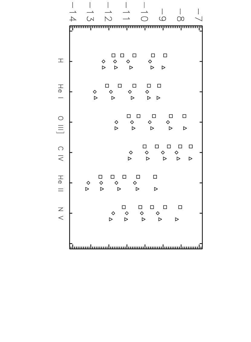
Figure 10:

Figure 11:

Figure 12:

Figure 13: