Late Spectral Evolution of SN 1987A:
I. Temperature and Ionization

Abstract

The temperature and ionization of SN 1987A is modeled between 200 and 2000 days in its nebular phase, using a time-dependent model. We include all important elements, as well as the primary composition zones in the supernova. The energy input is provided by radioactive decay of ${}^{56}\rm Co$, ${}^{57}\rm Co$, and ${}^{44}\rm Ti$. The thermalization of the resulting gamma-rays and positrons is calculated by solving the Spencer-Fano equation. Both the ionization and the individual level populations are calculated time-dependently. Adiabatic cooling is included in the energy equation. Charge transfer is important for determining the ionization, and is included with available and estimated rates. Full, multilevel atoms are used for the observationally important ions. As input models to the calculations we use explosion models for SN 1987A calculated by Woosley et al. and Nomoto et al.

The most important result in this paper refers to the evolution of the temperature and ionization of the various abundance zones. The metal-rich core undergoes a thermal instability, often referred to as the IR-catastrophe, at $600-1000$ days. The hydrogen-rich zones evolve adiabatically after $500-800$ days, while in the helium region both adiabatic cooling and line cooling are of equal importance after $\sim 1000$ days. Freeze-out of the recombination is important in the hydrogen and helium zones. Concomitant with the IR-catastrophe, the bulk of the emission shifts from optical and near-IR lines to the mid- and far-IR. After the IR-catastrophe, the cooling is mainly due to far-IR lines and adiabatic expansion.

Dust cooling is likely to be important in the zones where dust forms. We find that the dust condensation temperatures occur later than $\sim 500$ days in the oxygen-rich zones, and the most favorable zone for dust condensation is the iron core. The uncertainties introduced by the, in some cases, unknown charge transfer rates are discussed. Especially for ions of low abundances differences can be substantial.

1 INTRODUCTION

The observations of SN 1987A represent a unique set of data. Especially at late epochs high quality spectra exist at epochs when other supernovae are too faint to be observed even photometrically. This is particularly true for the IR region (e.g., Chevalier 1992, McCray 1993). The analysis of these observations are, however, not trivial and represent a considerably more complex situation compared to that of a planetary nebula, or an H II region. Complications include large optical depths of even forbidden lines, high velocities and consequent severe line blending, non-thermal excitation and ionization, non-uniform abundances, molecule and dust formation, as well as time-dependent effects. For reviews of the physics see McCray (1993) and Fransson (1994). In this paper and in Kozma & Fransson (1997) (Paper II) we concentrate on the spectral modeling in the nebular phase when the core region is transparent in at least the optical and IR regions. In a subsequent paper we will discuss the broad-band photometry, including the bolometric light curve.

Previous discussions of the late, nebular spectrum can be divided into attempts of self-consistent modeling of the spectrum, or analyses of the lines of particular elements or molecules. Models in the first category are hampered in many cases by lack of atomic data, as well as the general complexity of the problem. Examples of this type of models include some early predictions by Fransson & Chevalier (1987) and Colgan & Hollenbach (1988), and modeling of observed spectra by Swartz, Harkness, & Wheeler (1989). Applications to core collapse supernovae in general, including Type Ib’s and Type Ic’s can be found in Fransson & Chevalier (1989) and Swartz (1994). The ’diagnostic’ approach has been discussed in a series of papers by Li & McCray (1992, 1993, 1995), Li, McCray & Sunyaev (1993), Xu et al. (1992), Chugai (1994), and by Kozma & Fransson (1992, hereafter KF92). While the problem in this case is simplified to an easily controllable problem, it is often limited by the lack of knowledge of temperature, ionization and radiation field. As will be apparent in this paper and in Paper II, the limitation to one specific chemical composition, and in most cases a single element or ion, is especially severe.

Predictions are one of the best methods for judging the success of a complex model. It is therefore of some interest to discuss the paper by Fransson & Chevalier (1987), where immediately after the explosion predictions for the spectral evolution were made. There are several limitations to that paper. The most serious were the neglect of the hydrogen zone, and the simplified treatment of the iron emission. The model was therefore only applicable to the helium, oxygen and silicon – sulphur regions. Even with these limitations there were several interesting results. An important prediction in this paper was the dramatic drop in temperature at $\sim 600-700$ days in the metal-rich regions, and consequent transition from optical to far-IR radiation. This is commonly referred to as the IR-catastrophe (e.g., Axelrod 1980, Fransson 1994). The optical to far-IR transition is one of the characteristic features in the evolution of SN 1987A, and is clearly reflected if the light curves of the lines are plotted as a fraction of the total bolometric luminosity (e.g., Menzies 1991). Often this has been attributed to dust thermalization, which is certainly important, but independent of this, just the normal cooling in the metal-rich core will have this effect. The drop in temperature is also most likely a requirement for molecule and dust formation, and was in fact anticipated by Fransson & Chevalier. The concomitant drop in the optical lines and the dust formation, as seen in the line profiles (Lucy et al. 1989, 1991) and mid-IR emission (e.g., Wooden et al. 1993), are therefore most likely connected.

The predictions by Fransson & Chevalier have been directly compared to the observations of the light curves of the strongest lines, by Menzies (1991), Spyromilio et al. (1991), and Meikle et al. (1993). While there are quantitative discrepancies, it was found that the general shape of e.g. the strong [Ca II] $~{}\lambda~{}\lambda~{}7291,7324$ and [O I] $~{}\lambda~{}\lambda~{}6300,6364$ light curves agreed well qualitatively with the predictions. Note that most of the [Ca II] emission in this model comes from the oxygen-rich zone, and not from the calcium-rich Si – S zone, showing that a small amount of an effective cooler, like Ca II, can dominate the emission from a zone with a large gamma-ray deposition. In Paper II we will see that this is also the case in these models, although it is the hydrogen-rich zones, rather than the oxygen-rich wich dominate the emission, in agreement with Li & McCray (1993).

Another interesting result in the paper by Fransson & Chevalier was the non-uniform temperature and ionization in the different composition zones, with the metal-rich regions having considerably lower temperature. This illustrates the necessity to take all important abundance components into account, as well as the importance of distinguishing between macroscopic mixing of blobs of different compositions, compared to microscopic mixing of the gas.

An important aspect of the late evolution of the spectrum and light curve is the departure from (quasi-) steady state. As density decreases $\propto t^{-3}$, recombination and cooling time scales increase. Eventually, as these become longer than the radioactive decay time scale, $\tau$, the spectrum and light curve have to be calculated time-dependently. In addition, when the radiative cooling time becomes longer than the expansion time scale, adiabatic cooling must be included. These effects were discussed in Fransson & Kozma (1993), with particular emphasis on the consequences for the bolometric light curve. Implicit in this calculation was, however, a complete calculation of the spectrum as a function of time. Some results of this were reported in Fransson, Houck & Kozma (1996), and it was shown especially that the [O I] $~{}\lambda~{}\lambda~{}6300,6364$ lines provided compelling evidence for the IR-catastrophe. In addition, the importance of non-thermal excitation for the spectrum at late time were stressed. These points are discussed further in Paper II.

In these two papers we continue our attempt to model the evolution of the line emission from SN 1987A as realistically as possible. Consequently, we calculate the temperature and ionization self-consistently, using a time-dependent formalism. Non-thermal processes are included with the method in KF92. In addition, we include all important abundance zones in the ejecta with appropriate filling factors. The important ions are modeled as multilevel atoms, using the best available atomic data. Even with these ingredients there are a number of deficiencies in our modeling. Probably the most serious omission is that we do not include the resonance line blanketing, especially important in the UV. Further, the molecular chemistry and cooling are not included. Although we have tried to include the best atomic data available, we are still handicapped by a lack of reliable data, especially with regard to charge transfer reactions and photoionization of the iron group elements. In Paper II we argue that these omissions, although important for specific lines, should not influence our general conclusions severely. We hope to improve upon these shortcomings in the future.

In this paper we discuss our model and the temperature and ionization evolution in detail. In Paper II we concentrate on the line emission, as well as on the line profiles. In section  2 we discuss our basic model, assumptions, and physical processes included, as well as the explosion models we use. Section  3 contains a detailed discussion of our results with regard to the temperature and ionization, while in section  4 we discuss the sensitivity of our results to especially the UV-radiation field and the poorly known charge transfer rates. In section  5 we discuss the dust formation and the effects of dust cooling. In section 6 our main results are for convenience summarized. In the appendix we have collected the references for the atomic data.

2 THE MODEL

In these papers we focus on the emission from SN 1987A at times later than $\sim$ 200 days, when the supernova has entered the nebular phase. As the matter is expanding and becoming more transparent, it is possible to extract information on the nucleosynthesis, which has taken place in the progenitor and in the explosion, as well as on the hydrodynamics of the explosion.

Our model calculates the temperature, ionization and level populations of the different regions in the supernova envelope. The first time step is calculated in steady state, which is a good approximation at 200 days. The following time steps are calculated time-dependently. Knowing the time evolution of the physical properties of the supernova matter we calculate the bolometric luminosity, as well as luminosities for $\sim 5900$ lines. As input, the calculations require an explosion model, as well as the radial structure of the ejecta with abundances and masses as a function of velocity. Our model is spherical symmetric, with zones of different compositions and thicknesses. Mixing in velocity is taken into account in an approximate way by mixing shells from different abundance zones in velocity.

We have the option to switch between either doing the calculations in steady state or time-dependently. The steady state calculations are done primarily in order to check that energy is conserved at every time step. We find that energy is conserved to within $\sim$ 1 % at all times. By comparing the steady state and time-dependent calculations it is possible to determine the level of freeze-out. The temperature, ionization, and level populations of the multi-level atoms are calculated time-dependently.

Below, we first discuss the physical processes included in our model, and then the explosion models used in our calculations.

2.1 Physical Processes

2.1.1 Temperature Calculation

The temperature, $T$, of a region is determined by balancing the cooling and heating mechanisms. In steady state the total cooling ($\Lambda nn_{e}$) at a certain point is just balanced by the total heating ($H$),

$$\Lambda(T)nn_{e}=H.$$ (1)

From this condition it is possible to determine the temperature. In the time-dependent case the temperature change can be expressed as

$$\frac{dT}{dt}=\frac{2}{3k(1+x_{e})n}(H-\Lambda(T)nn_{e})-\frac{2T}{t}-\frac{T}{1+x_{e}}\frac{dx_{e}}{dt}$$ (2)

where $n$ is the number density of ions and atoms, $n_{e}$ the number density of free electrons, and $x_{e}=n_{e}/n$. The second term in this equation describes adiabatic cooling. If this term dominates, $T\propto t^{-2}$.

Most of the cooling is by collisional excitation of bound-bound transitions. The total line cooling is a sum over all the transitions $i,j$,

$$L_{\rm lines}=\sum_{i,j}(n_{i}n_{e}C_{ij}(T)-n_{j}n_{e}C_{ji}(T))h\nu_{ij}\hskip 28.45274pt,$$ (3)

where $C_{ij}(T)$ and $C_{ji}(T)$ are the collisional excitation, and de-excitation rates, respectively (Osterbrock 1989), $n_{i}$ is the number densities of ions in level $i$, and $h\nu_{ij}$ is the photon energy. Line cooling is the dominant cooling process, but we also include cooling due to recombinations and free-free cooling. We approximate recombination cooling with

$$L_{\rm rec}\approx\sum_{k}n_{k+1}n_{e}\alpha_{k}kT\hskip 28.45274pt,$$ (4)

where the summation is over all ions $k$, and $\alpha_{k}$ refers to the recombination from $k+1$ to $k$.

Free-free cooling is given by

$$L_{\rm ff} = \sum_{k}1.426\times 10^{-27}T^{1/2}Z_{k}^{2}n_{e}n_{k}<g_{\rm ff}>.$$ (5)

The summation is over the ions $k$, $Z_{k}$ is the charge of ion $k$, and $<g_{\rm ff}>$ is the mean gaunt factor for free-free emission.

Cooling, both due to lines, recombinations, and free-free emission, is in the low density, optically thin limit, proportional to the electron fraction. We therefore define a cooling function, $\Lambda(T)$, so that the total cooling equals $\Lambda(T)nn_{e}=L_{\rm lines}+L_{\rm rec}+L_{\rm ff}$,

$$\Lambda(T) = \sum_{k}[\sum_{ij}(x_{i}C_{ij}(T)-x_{j}C_{ji}(T))h\nu_{ij}+$$ (7)

$${3\over 2}x_{k+1}\alpha_{k}kT+1.426\times 10^{-27}T^{1/2}Z_{k}^{2}x_{k}<g_{\rm ff}>]\hskip 28.45274pt,$$

where $x_{i}$ is the fraction of ions in level $i$, and the summation over $k$ represents all ions. $\Lambda$ depends sensitively on the electron temperature, $T$.

The heating in the ejecta is dominated by non-thermal heating, $H_{\gamma}$, which is independent of the electron temperature. This process is discussed in detail in KF92. We express the non-thermal heating as

$$H_{\gamma}=4\pi J_{\gamma}\sigma_{\gamma}\eta_{\rm H}n\hskip 28.45274pt,$$ (8)

where $4\pi J_{\gamma}\sigma_{\gamma}$ is the deposited non-thermal energy per particle. This quantity is discussed in more detail below. $\eta_{\rm H}$ is the fraction of the deposited energy going into heating the free, thermal electrons. $\eta_{\rm H}$ depends on the electron fraction, and increases with increasing $x_{e}$ (KF92).

Photoelectric heating from the ground states is included for all ions $k$, and from excited levels $i$, where there is atomic data available. The total photoelectric heating can be expressed,

$$H_{\rm P}=\sum_{k}\sum_{i}\hskip 8.5359ptn_{k,i}\int_{\nu_{k,i}}^{\infty}4\pi\frac{\sigma_{\nu}J_{\nu}(h\nu-\chi_{k,i})}{h\nu}d\nu\hskip 28.45274pt,$$ (9)

where $h\nu_{k,i}$ is the ionization energy, $\sigma_{\nu}$ is the photoionization cross section from level $i$ in ion $k$, $J_{\nu}$ is the mean radiation intensity at $\nu$, and $\chi_{k,i}$ is the ionization potential.

The total heating is therefore

$$H=H_{\gamma}+H_{\rm P}\hskip 28.45274pt.$$ (10)

2.1.2 Ionization Balance

In our calculations we include H I-II, He I-III, C I-III, N I-II, O I-III, Ne I-II, Na I-II, Mg I-III, Si I-III, S I-III, Ar I-II, Ca I-III, Fe I-V, Co II, and Ni I-II.

For an estimated value of the electron fraction, $x_{e}$, the ionization balance for an element with only two ionization stages, $k$ and $k+1$ is solved from

$$\frac{dn_{k}}{dt}+\frac{3n_{k}}{t} = -(\Gamma_{k}+P_{k})n_{k}-n_{k}\sum_{l}n_{l}\xi^{\rm CT}_{k,l}+$$ (12)

$$\alpha_{k}n_{e}n_{k+1}+n_{k+1}\sum_{l}n_{l}\xi^{\rm CT}_{k+1,l}.$$

For elements with three or more ionization stages equation (12) is generalized to include processes both below and above the relevant ionization stage. Here, $\Gamma_{k}$ is the non-thermal ionization rate,

$$\Gamma_{k}=4\pi\frac{J_{\gamma}\sigma_{\gamma}}{\chi_{eff,k}}\hskip 28.45274pt,$$ (13)

where $\chi_{eff,k}$ is the effective ionization potential, defined as $\chi_{eff,k}=\chi_{k}x_{k}/\eta_{k}$ (see KF92), $\chi_{k}$ being the ionization potential, $x_{k}$ the number fraction, and $\eta_{k}$ the fraction of the deposited non-thermal energy going into ionization of ion $k$. $P_{k}$ is the photoionization rate,

$$P_{k}=4\pi\int_{\nu_{0}}^{\infty}\frac{\sigma_{k,\nu}J_{\nu}}{h\nu}d\nu\hskip 28.45274pt,$$ (14)

while $\alpha_{k}$ is the recombination coefficient from $k+1$ to $k$. In our calculations $P_{k}$ and $\alpha_{k}$ include photoionizations from, and recombinations to excited levels in ion k.

In many cases charge transfer reactions with ions $l$ may contribute, either as an ionization, $n_{k}n_{l}\xi^{\rm CT}_{k,l}$, or recombination, $n_{k+1}n_{l}\xi^{\rm CT}_{k+1,l}$, process (Fransson & Chevalier 1989, Swartz 1994). Excited levels of ion $k$ may also be involved.

Finally, the number conservation equation is

$$\sum_{k}n_{k}=n_{\rm element}.$$ (15)

Equations (12) and (15) are solved using the Newton-Raphson method. For stability and efficiency, equations (12) and (15) are solved implicitly with backward differencing,

$$\frac{n_{k}^{n+1}-n_{k}^{n}}{\Delta t}=f(n_{k}^{n+1})$$ (16)

where $n_{k}^{n+1}$ refers to the new value and $n_{k}^{n}$ to the old value. The function $f(n_{k}^{n+1})$ on the right hand side includes all ionization and recombination processes in equation (12). Even though the implicit treatment requires iteration, it makes the overall problem more stable, and allows considerably longer time steps. The time step varies between the different zones, depending on the cooling and recombination time scales. The hydrogen and helium-rich regions therefore require smaller number of time steps, compared to the metal-rich regions, where these time scales are short. For the same reason, the late stages allow longer time steps, compared to the first epochs. As an example, the iron zones require $\sim 15000$ time steps from 200 – 2000 days, while the corresponding numbers are $\sim 4000$ for the oxygen zones, and $\sim 1000$ for the hydrogen zones.

2.1.3 Level Populations

With the abundance of each ionization stage known, the level populations are calculated for a number of ions. For the following multilevel atoms we calculate the level populations time-dependently : H I  (30 levels with $n\leq 20$), He I  (16 levels), O I  (13 levels), Ca II  (6 levels), Fe I  (121 levels), Fe II  (191 levels), Fe III  (110 levels), and Fe IV  (43 levels). Lines from other elements are solved, either as two-level atoms, or, in the case of forbidden lines, as 4-6 level systems (see appendix).

The rate equations for the level populations are given by

$$\frac{dn_{k,i}}{dt}+\frac{3n_{k,i}}{t} = -n_{k,i}(P_{k,i}+\Gamma_{k,i}+\alpha_{i,k-1}n_{e})$$ (31)

$$-n_{k,i}\sum_{j<i}(A_{ij}\beta_{ij}+C_{ij}n_{e}+P_{ij})$$

$$+\sum_{j<i}n_{k,j}(C_{ji}n_{e}+\Gamma_{ji}+P_{ji})$$

$$-n_{k,i}\sum_{j>i}(C_{ij}n_{e}+\Gamma_{ij}+P_{ij})$$

$$+\sum_{j>i}n_{k,j}(A_{ji}\beta_{ji}+C_{ji}n_{e}+P_{ji})$$

$$+n_{k+1}\alpha_{k,i}n_{e}+n_{k-1}(P_{i,k-1}+\Gamma_{i,k-1})$$

$$-n_{k,i}\sum_{l}n_{l}\xi^{\rm CT}_{k,l}+n_{k+1}\sum_{l}n_{l}\xi^{\rm CT}_{k+1,l}$$

$$+n_{k-1}\sum_{l}n_{l}\xi^{\rm CT}_{k-1,l}$$

where the index $i$ refers to the actual level, and $j$ to other levels within the ion, $k$ to the ionization stage of the element, and $l$ to any other element. $P_{k,i}$ and $\Gamma_{k,i}$ are the photoionization rate and non-thermal ionization rate, from ion $k$, level $i$. $\alpha_{i,k-1}$ is the recombination coefficient from ion $k$, and level $i$ to ion $k-1$. Downward and upward radiative, and collisional rates, $A_{ij}\beta_{ij}$ and $C_{ij}n_{e}$, are included. Here $\beta_{ij}$ is the escape probability, which includes both the Sobolev escape probability and a continuum destruction probability. This is discussed in more detail in sections 2.1.5 and  2.1.6.

Similar to the non-thermal ionization rate (eq. [13]) the non-thermal excitation rate $\Gamma_{ij}$ from the lower level $i$ to the upper level $j$ is given by

$$\Gamma_{ij}=\frac{4\pi J_{\gamma}\sigma_{\gamma}}{\chi_{ij}x_{i}/\eta_{ij}}\hskip 28.45274pt,$$ (32)

where $\chi_{ij}$ is the excitation energy, $x_{i}$ the number fraction in level $i$, and $\eta_{ij}$ is the fraction of the deposited energy going into excitation of the transition $ij$. For those elements where non-thermal excitations are included, only excitations from the ground state, $i=1$, are calculated except for O I, Fe I  and Fe II. For these, non-thermal excitations from the individual levels of the ground state multiplet are included.

$P_{ij}$ and $P_{ji}$ are the photoexcitation/deexcitation rates between levels $i$ and $j$. The Einstein relations and the Sobolev assumption (e.g., Tielens & Hollenbach 1985) result in

$$P_{ji}=\frac{c^{2}}{2h\nu^{3}}A_{ji}\beta_{ji}J_{ji}$$ (33)

and

$$P_{ij}=\frac{g_{j}}{g_{i}}P_{ji}.$$ (34)

In accordance to our neglect of line blanketing, we only include the continuum contribution to $J_{ji}$ (see section 2.1.7). Further, $\alpha_{k,i}$ is the recombination coefficient from ion $k+1$ to an individual level $i$ of ion $k$. For ions once or more ionized, photoionization and non-thermal ionization from ion $k-1$ are included. We assume that these ionizations end up in the first level, $i=1$, $P_{i=1,k-1}$ and $\Gamma_{i=1,k-1}$, with the exception of O II. For oxygen we include non-thermal ionization from O I to the excited states ${}^{2}D_{o}$ and ${}^{2}P_{o}$, as well as to the ground state of O II.

Charge transfer reactions with other elements may either act as an ionization or recombination process. We assume that charge transfer reactions occur from their ground states, $i=1$, with the exception for He I. Swartz (1994) gives rates for charge transfer involving excited levels in He I. The term $n_{k}n_{l}\xi^{\rm CT}_{k,l}$ represents the charge transfer rate for the reaction $A^{k}+B^{l}\rightarrow A^{k\pm 1}+B^{l\mp 1}$, and $n_{k\pm 1}n_{l}\xi^{\rm CT}_{k\pm 1,l}$ the charge transfer rate for the reaction $A^{k\pm 1}+B^{l}\rightarrow A^{k}+B^{k\pm 1}$. Charge transfer reactions are further discussed in section 2.1.8.

Together with the particle conservation equation

$$n_{k}=\sum_{i}n_{k,i},$$ (35)

the rate equations are again solved implicitly, using Newton-Raphson iteration.

2.1.4 Non-Thermal Deposition

The energy source for the ejecta at late times is well established to be the decay of radioactive isotopes created in the explosion. The dominant isotope synthesized is ${}^{56}\rm Ni$. ${}^{56}\rm Ni$ rapidly decays to ${}^{56}\rm Co$ on a time scale of $\tau_{\rm decay}$ = 8.8 days. ${}^{56}\rm Co$ then decays to ${}^{56}\rm Fe$ on a longer time scale of 111.26 days. In the decay of ${}^{56}\rm Co$ 96.5 % of the energy is emitted in the form of gamma-rays while the remaining 3.5 % of the energy is emitted as positrons. Other important radioactive isotopes created in the explosion are ${}^{57}\rm Ni$ and ${}^{44}\rm Ti$. ${}^{57}\rm Ni$ decays rapidly to ${}^{57}\rm Co$, and ${}^{57}\rm Co$ to ${}^{57}\rm Fe$ with $\tau_{\rm decay}$ = 391.2 days. Decays of ${}^{57}\rm Co$ only result in gamma-rays, no positrons. ${}^{44}\rm Ti$ decays first to ${}^{44}\rm Sc$ on a time scale of 83.7 years followed by a rapid decay to ${}^{44}\rm Ca$. In the decay of ${}^{44}\rm Sc$ positrons are also emitted.

The gamma-ray luminosity due to the decay of ${}^{56}\rm Co$ is

$$L_{\gamma}=1.26\times 10^{42}\frac{M(\hbox{${}^{56}\rm Ni$})}{0.1{~{}\rm M}_{\odot}}e^{-t/111.26^{d}}\hskip 28.45274pt{\rm erg~{}s^{-1}}$$ (36)

of ${}^{57}\rm Co$,

$$L_{\gamma}=1.37\times 10^{41}M(\hbox{${}^{57}\rm Ni$})e^{-t/391.2^{d}}\hskip 28.45274pt{\rm erg~{}s^{-1}},$$ (37)

and of ${}^{44}\rm Ti$,

$$L_{\gamma}=4.1\times 10^{36}\frac{M(\hbox{${}^{44}\rm Ti$})}{10^{-4}{~{}\rm M}_{\odot}}e^{-t/83.7^{yr}}\hskip 28.45274pt{\rm erg~{}s^{-1}}.$$ (38)

These expressions include the gamma-rays due to positron annihilation.

Positrons are assumed to be deposited locally in the iron-rich regions. This is supported even at 7.8 years by the analysis of the spectrum of SN 1987A by Chugai et al. (1997). The luminosity due to the energy input from positrons from ${}^{56}\rm Co$ decay is

$$L_{e^{+}}=3.34\times 10^{40}\frac{M(\hbox{${}^{56}\rm Ni$})}{0.075{~{}\rm M}_{\odot}}e^{-t/111.26^{d}}\hskip 28.45274pt{\rm erg~{}s^{-1}}$$ (39)

and from ${}^{44}\rm Ti$,

$$L_{e^{+}}=1.3\times 10^{36}\frac{M(\hbox{${}^{44}\rm Ti$})}{10^{-4}{~{}\rm M}_{\odot}}e^{-t/83.7^{yr}}\hskip 28.45274pt{\rm erg~{}s^{-1}}.$$ (40)

The life time of ${}^{44}\rm Ti$ is uncertain, with values ranging from 66.9 – 96.1 years (see Timmes et al. 1996). Here we use the latest value of $83.7\pm 15$ years (Meissner et al. 1995). In our calculations we include 0.07 ${~{}\rm M}_{\odot}$ of ${}^{56}\rm Ni$, from the bolometric light curve, $3.3\times 10^{-3}{~{}\rm M}_{\odot}$ of ${}^{57}\rm Ni$, which corresponds to a ${}^{57}\rm Ni$/${}^{56}\rm Ni$ ratio equal to 2 times the solar ${}^{57}\rm Fe$/${}^{56}\rm Fe$ ratio, and $10^{-4}{~{}\rm M}_{\odot}$ of ${}^{44}\rm Ti$ (Woosley, Pinto & Weaver 1988, Kumagai et al. 1991, Woosley & Hoffman 1991). These masses correspond to our standard case in Fransson & Kozma (1993). With these masses, ${}^{56}\rm Co$ dominates the energy input up to $\sim$ 1200 days. Thereafter, ${}^{57}\rm Co$ takes over up to $\sim$ 1900 days, after which ${}^{44}\rm Ti$ dominates. ²²Na with a decay time of 3.75 years never contributes more than 10 % before 2000 days (Woosley, Pinto & Hartman 1989).

Thermalization of the gamma-rays and positrons is discussed in detail in KF92 and Li, McCray, & Sunyaev (1993). Using the Spencer-Fano formalism (e.g., Spencer & Fano 1954, Douthat 1975a,b, Xu 1989) we calculate the fractions of the deposited energy going into heating, ionization, and excitation, respectively. These fractions depend on the composition of the gas, the state of ionization and the electron fraction. The Spencer-Fano calculations are repeated for each composition zone, when the electron fraction has changed by more than 5 %, or by more than 0.01 in absolute value.

The gamma-ray intensity depends on the distribution of the radioactive elements. This is uncertain, and depends on the degree of mixing in the gas (see section  2.2). We distribute the radioactive source within the core, proportional to the iron mass. The ionization, excitation, and heating depend on $4\pi J_{\gamma}\sigma_{\gamma}$ (${\rm erg~{}s^{-1}~{}particle^{-1}}$), the total gamma-ray energy deposited per second per particle at a certain radius in the supernova ejecta. With particles we refer to ions and atoms (not electrons). $J_{\gamma}(r)$ is the gamma-ray mean intensity at radius $r$, $\sigma_{\gamma}(r)$ (${\rm cm^{2}~{}particle^{-1}}$) is the energy-averaged cross section for gamma-ray absorption at radius $r$ for an ion. For the gamma-rays resulting from the decay of ${}^{56}\rm Co$, Fransson & Chevalier (1989) find $\kappa_{\gamma}=0.06~{}(Z_{i}/A_{i})~{}{\rm cm^{2}~{}g^{-1}}$, where $Z_{i}$ and $A_{i}$ is the nuclear charge and the atomic weight, respectively, for ion $i$. For hydrogen-rich regions $Z_{i}/A_{i}\approx 1$, while in the other regions, dominated by helium or heavier elements, $Z_{i}/A_{i}\approx 0.5$. Therefore, we use $\kappa_{\gamma}(\hbox{${}^{56}\rm Co$})=0.06~{}{\rm cm^{2}~{}g^{-1}}$ in the hydrogen-rich regions, and $\kappa_{\gamma}(\hbox{${}^{56}\rm Co$})=0.03~{}{\rm cm^{2}~{}g^{-1}}$ in the remaining regions. The average cross section for a particular composition is then calculated from $\sigma_{\gamma}(\hbox{${}^{56}\rm Co$})=A_{\rm mean}~{}m_{p}~{}\kappa_{\gamma}(\hbox{${}^{56}\rm Co$})$, where $A_{\rm mean}$ is the mean atomic weight in the region.

The mean energy of the gamma-rays emitted in the ${}^{57}\rm Co$-decay is lower than in the decay of ${}^{56}\rm Co$. Woosley et al. (1989) find that $\kappa_{\gamma}(\hbox{${}^{57}\rm Co$})\approx 2.4~{}\kappa_{\gamma}(\hbox{${}^{56}\rm Co$})$, and also an effective opacity for the gamma-rays from ${}^{44}\rm Ti$, $\kappa_{\gamma}(\hbox{${}^{44}\rm Ti$})=0.040$, compared to $\kappa_{\gamma}(\hbox{${}^{56}\rm Co$})=0.033$. In our calculations we use the the same opacity for ${}^{44}\rm Ti$ and ${}^{56}\rm Co$.

In the case of a central energy source the total deposited energy may be calculated from,

$$4\pi\sigma_{\gamma}J_{\gamma}(r) = [(1-e^{-\Delta\tau_{\gamma,56}(r)})e^{-\tau_{\gamma,56}(r)}L_{\gamma,56}+$$ (45)

$$(1-e^{-\Delta\tau_{\gamma,57}(r)})e^{-\tau_{\gamma,57}(r)}L_{\gamma,57}+$$

$$(1-e^{-\Delta\tau_{\gamma,44}(r)})e^{-\tau_{\gamma,44}(r)}L_{\gamma,44}]/n_{\rm ion}(r),$$

where the index 56 refers to ${}^{56}\rm Co$, 57 to ${}^{57}\rm Co$, and 44 to ${}^{44}\rm Ti$, the quantity $\tau(r)$ is given below in equation (53), $\Delta\tau(r)=\sigma(r)n(r)\Delta r$ is the optical depth of the shell of thickness $\Delta r$, and $n_{\rm ion}(r)$ is the number of particles (i.e. ions) at $r$.

If the radioactive isotopes are distributed throughout the core region, the calculation of $J_{\gamma}$ is more complicated. Knowing the luminosities for the radioactive isotopes (eqs. [36] - [38]), and their distribution (from the explosion model) we find the emissivity as a function of radius, $j_{\gamma}(r)$ We then calculate the total deposited energy from

$$4\pi\sigma_{\gamma}J_{\gamma}(r) = 4\pi\frac{1}{2}\int_{-1}^{1}\int_{0}^{l_{\rm max}(\mu)}[\sigma_{\gamma,56}(r)j_{\gamma,56}(l)e^{-\tau_{\gamma,56}(l)}$$ (52)

$$+\sigma_{\gamma,57}(r)j_{\gamma,57}(l)e^{-\tau_{\gamma,57}(l)}$$

$$+\sigma_{\gamma,44}(r)j_{\gamma,44}(l)e^{-\tau_{\gamma,44}(l)}]~{}dl~{}d\mu.$$

For each $r$, inside the core ($r<R_{\rm core}$), we integrate over all angles, $\mu=\cos\theta$, integration interval [-1,1]. For each $\mu$ we integrate along a path, $l$, from $r$ ($l=0$) to the border of the core region, $R_{\rm core}$ ($l=l_{\rm max}$). Outside of the core ($r>R_{\rm core}$) the integration interval for $\mu$ is [-1,-$\sqrt{r^{2}-R_{\rm core}}/r$]. The optical depth, $\tau$, in equation (52) is given by

$$\tau(l)=\int_{0}^{l}\sigma(l^{\prime})n(l^{\prime})dl^{\prime},$$ (53)

for each isotope.

In general we can write

$$J_{\gamma}=\frac{L_{\gamma}D_{\gamma}}{16\pi^{2}R_{\rm core}^{2}},$$ (54)

where $R_{\rm core}$ is the core radius. Limiting forms of $D_{\gamma}$ are discussed in KF92.

2.1.5 Line Transfer

In our calculations we take the radiative transfer of the lines into account by using the Sobolev approximation (Sobolev 1957, 1960, Castor 1970). The supernova ejecta is expanding homologously at the times we are interested in. Therefore, each mass element, with mass coordinate $M$, has a constant velocity, $v(M)=$ constant, or $r(M)=v(M)t$, where $t$ is the time since core collapse. The expansion velocity is much larger than the thermal velocity of the matter, and the Sobolev approximation is therefore valid for an individual, well separated line. With this approximation the line transfer becomes a purely local phenomena, either the photon is re-absorbed locally or escapes the medium. A photon emitted in a certain transition may, however, be absorbed by a line with a longer wavelength at a different point in the ejecta. This line blocking is important in the UV, and we hope to treat this in a subsequent paper (see also Fransson 1994, Li & McCray 1996, Houck & Fransson 1996). The effect of this has been checked by comparing calculations for SN1993J (Houck & Fransson 1996) with and without these processes included, where it was found that the strongest lines from dominant ions with high ionization potentials, like O I, were only slightly affected, while elements with low ionization potentials and low abundances, like Na I, are sensitive to the UV-field. The electron density and temperature were only marginally affected. We test the sensitivity of our results to the UV-field by having the option of switching it on or off. This is discussed in Paper II. Our crude treatment of the radiative transfer is one of the major weaknesses of our calculations.

The Sobolev escape probability, $\beta_{\rm s}$, can be written

$$\beta_{\rm s}=\frac{1-e^{-\tau_{\rm s}}}{\tau_{\rm s}}.$$ (55)

Here $\tau_{\rm s}$ is the Sobolev optical depth for a particular transition, $ij$ ($i<j$),

$$\tau_{\rm s}=\frac{A_{ji}n_{i}\lambda_{0}^{3}}{8\pi}\frac{g_{j}}{g_{i}}t(1-\frac{g_{i}}{g_{j}}\frac{n_{j}}{n_{i}})$$ (56)

In addition of being re-absorbed in the line itself, a line photon may also be destroyed by continuum absorption, i.e., photoionization. Note that the Sobolev expression for the escape probability (eq. [56]) is independent of assumptions of the line profile (e.g., Rybicki 1984).

2.1.6 Continuum Destruction

The continuum destruction probability, $\beta_{\rm c}$, has in the Sobolev approximation been calculated by Hummer & Rybicki (1985) for the Doppler case and complete redistribution,

$$\beta_{\rm c}\approx{k_{\rm C}\over k_{\rm L}}F(\xi,{k_{\rm C}\over k_{\rm L}}).$$ (57)

In this equation $k_{\rm C}/k_{\rm L}$, is the ratio between the continuum opacity, $k_{\rm C}$, and the line core opacity, $k_{\rm L}$, and $\xi=1/\tau_{\rm s}$. For a Doppler profile Hummer & Rybicki (1985) approximate $F(\xi,{k_{\rm C}\over k_{\rm L}})$ by

$$F(\xi,{k_{\rm C}\over k_{\rm L}})\approx 2\{-\ln\surd\pi({k_{\rm C}\over k_{\rm L}}+2\xi[-\ln\surd\pi({k_{\rm C}\over k_{\rm L}}+2\xi x_{0})]^{1/2})\}^{1/2},$$ (58)

where $x_{0}\approx 2$ is the frequency displacement from the line center in thermal Doppler widths, $(\nu-\nu)/\Delta\nu_{\rm D}$. The assumptions made for this estimate are that $k_{\rm C}/k_{\rm L}\ll 1$ and $\xi\ll 1$.

For strong resonance lines the damping wings may become important. In this case the continuum destruction probability above is modified. The destruction probability in the Voigt case with $\it complete$ redistribution has for a static geometry been calculated by Hummer (1968), giving expressions and tabulations for the function $F$ above. For $k_{\rm C}/k_{\rm L}\lesssim 0.1a$ and $a\lesssim 0.1$, where $a$ is the damping parameter, Hummer gives the approximation

$$F(\xi,{k_{\rm C}\over k_{\rm L}})\approx\left({\pi~{}a~{}k_{\rm L}\over k_{\rm C}}\right)^{1/2}.$$ (59)

For $k_{\rm C}/k_{\rm L}\gtrsim 0.1a$ equation (58) gives an adequate approximation.

The validity of complete redistribution versus partial redistribution has been discussed extensively for solar conditions in the case of ${\rm Ly}\alpha$, Ca II H & K and Mg II (e.g., Mihalas 1978, and references therein). It is there concluded that at densities lower than those prevailing in the outer chromosphere, partial redistribution is a better approximation to the line profile in the damping wings of the lines. Because the densities are in our case considerably lower than this, it is likely that partial redistribution is a more realistic assumption for the strong resonance lines from the ejecta. The continuum destruction has for partial redistribution been discussed by Chugai (1987), who finds the approximation

$$F(\xi,{k_{\rm C}\over k_{\rm L}})\approx 1.87~{}\left({a~{}k_{\rm L}\over k_{\rm C}}\right)^{1/4}.$$ (60)

This expression takes only scattering in the wings into account, and does not apply to the Doppler core, where complete redistribution, as given by equation (58), is adequate.

The most important lines for which partial redistribution applies are ${\rm Ly}\alpha$, He I $~{}\lambda~{}584$, Ca II H and K, O I $~{}\lambda~{}1302$, and Mg II $~{}\lambda~{}2800$, as well as the Fe II resonance lines. As will be seen in Paper II, the choice of destruction probability has important effects for especially the He I $~{}\lambda~{}584$ line and the branching to the $~{}\lambda~{}2.058~{}\mu$m line. The effects of this are discussed in Paper II.

In our calculations we use the effective transition probability, $A_{ji}\beta_{ji}$ where the escape probability $\beta_{ji}$ includes both the Sobolev escape probability, and the continuum destruction probability,

$$\beta_{ji}=(1-\beta_{\rm c})\beta_{\rm s}+\beta_{\rm c}.$$ (61)

2.1.7 Photoionization and Photoexcitation/deexcitation

In our calculation of the ionization balance we include photoionization of all the ions with ionization potential smaller than 30 eV. Where data is available, we also include photoionization from excited levels in our multi-level atoms. Lines, recombination emission, two-photon emission and free-free emission may contribute to the photoionization.

We assume that only the continuum emission (recombination, two-photon, and free-free emission) contribute to the photoexcitation/deexcitation. Line photons destroyed by continuum absorption (see previous section) are added to the photoionization of the different elements, according to their fractional opacity. References for the photoionization cross sections are given in the appendix.

2.1.8 Charge Transfer and Penning Ionization

Charge transfer reactions may be important in determining the ionization stages for the elements (Fransson 1994, Swartz 1994). This is especially the case for trace elements. The ionization balance of the dominating element in a zone is, however, not affected much by charge transfer reactions. Therefore, the total electron fraction is rather insensitive to these reactions. References to the sources of data are given in the appendix.

In modeling the helium emission from SN 1987A the Penning ionization process,

$$\begin{array}[]{lllllllll}{\rm He\,I}~{}(2^{3}S)&+&{\rm H\,I}&\rightarrow&{\rm He\,I}~{}(1^{1}S)&+&{\rm H\,II}&+&e^{-}\end{array}$$ (62)

may be important for de-populating the excited level $2^{3}S$ of He I  (Chugai 1991, Li & McCray 1995). We include this process in our model.

2.2 The Explosion Model

As input to our calculations we require a model for the composition and mass (or equivalently, the density) as a function of velocity. The assumption of homologous expansion relates the radius of a mass element to the velocity, $r(M)=v(M)t$. Explosion models for SN 1987A have been calculated by Nomoto & Hashimoto (1988), Woosley (1988), Arnett (1987), and Hashimoto, Nomoto, & Shigeyama (1989). These models are all one-dimensional calculations. However, several groups have found that the core is unstable to hydrodynamical instabilities, causing mixing of the various burning shells, as well as modifying the density distribution (e.g., Fryxell, Müller, & Arnett 1991, Hachisu et al. 1992, Herant & Benz 1991, 1992). This mixing should be macroscopic, with little mixing on the microscopic scale (Fryxell et al. 1991). As emphasized by e.g. Fransson & Chevalier (1989) and Li, McCray & Syunyaev (1993), macroscopic mixing, rather than microscopic, can have a major influence on the observed spectrum.

In our calculations we assume an overall spherical symmetry, with shells of different compositions and masses. Unfortunately, most models which treat the nucleosynthesis in sufficient detail are completely one-dimensional, with shells containing the heavy elements close to the center, and with continuously decreasing mean atomic weight as one proceeds outward in radius. Conversely, multi-dimensional models start with artificial initial perturbations, and do not treat the nucleosynthesis in detail. Because of limited computing power it is also not yet realistic to include multi-dimensional effects in the calculation of the spectrum, especially with regard to the radiative transfer.

For these reasons we mimic the macroscopic mixing by using the results of the one-dimensional explosion models with regard to the nucleosynthesis, but not in density and velocity. Instead, we divide the ejecta into a core region, containing the metal-rich region, and where mixing is determining the distribution in velocity, and an envelope, containing most of the hydrogen, as well as a major part of the helium, and where mixing is less important. To simulate the structure of the multi-dimensional models in the core we divide this into a number of shells with varying compositions, placed in an alternating order. The density, $\rho_{i}$, of each of these shells is determined by the total mass of the component in the core, $M_{i}$, and its filling factor, $f_{i}$, so that

$$\rho_{i}={3~{}M_{i}\over 4\pi~{}f_{i}~{}V_{\rm core}^{3}~{}t^{3}}.$$ (63)

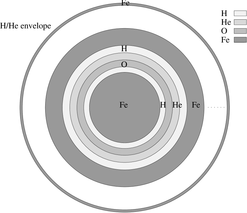
Figure 1: Schematic figure showing the model structure of the ejecta, where the thickness of the zones correspond to the filling factors of the shells. We have for clarity omitted the O – C and Si – S zones, as well as the various zones in the envelope. In the white zone between the second and third iron zones we have an additional set of O, He, H, Fe, O, He, and H zones. The inner hydrogen zone and the outermost iron zone, which break the regularity, have been added to produce the correct line profiles.

Each component is then divided into a number of shells, usually three, all having this density, placed uniformly within the core. In some cases (see below) we determine the location, and masses of these shells, so that a best fit to the line profiles is obtained. A schematic representation of the structure, including only a few of the zones, is given in Figure 1.

Based on line widths of [O I], Mg I], and [Fe II] lines we take the velocity of the core to be $2000\rm~{}km~{}s^{-1}$. The structure of the envelope is based on the line profiles of ${\rm H}\alpha$ and the He I $~{}\lambda~{}2.058~{}\mu$m line (Paper II). In our calculations we use a maximum expansion velocity for the envelope of $6000\rm~{}km~{}s^{-1}$.

To represent the most important burning zones in the post-explosion ejecta we include six different abundance components. The dominant elements (by number) are Fe – He, Si – S, O – Si – S/O – Ne – Mg, O – C, He, and H. Abundances are either from the 10H model (Woosley & Weaver 1986, Woosley 1988) or the 11E1 model (Nomoto, & Hashimoto 1988, Shigeyama, Nomoto, & Hashimoto 1988, Shigeyama & Nomoto 1990, Hashimoto et al. 1989). The abundances used, together with the masses of the different components, for the 10H and 11E1 models are presented in Tables 1 and 2. The sodium abundance is not given in the 10H model. We estimate this by scaling it from the magnesium abundance, so that the integrated $X(\hbox{${}^{23}\rm Na$})/X(\hbox{${}^{24}\rm Mg$})$ ratio is that given by the 11E1 model. This gives $X({\rm Na})\approx 8.2\times 10^{-3}~{}X({\rm Mg})$. The mass of synthesized stable nickel, M(⁵⁸Ni)$+$ M(⁶⁰Ni) $=0.006{~{}\rm M}_{\odot}$, is from Nomoto et al. (1991). The abundances in the hydrogen-rich component in SN 1987A are based on modeling of the circumstellar ring by Lundqvist & Fransson (1996), with C:N:O = 1:5:4, by number. For sodium, magnesium, argon, and calcium we use 0.4 times the cosmic abundance in the hydrogen-rich zones, and LMC abundances of Fe (Russell & Dopita, 1992). The stable nickel abundance is determined from the Ni/Fe ratio in LMC from Russell & Dopita (1992). For stable cobalt, the solar abundance ratio, Co/Fe, from Anders & Grevesse (1989) is used. The explosion models only include synthesized elements. Therefore, if the abundance given by the explosive model is smaller than the LMC abundance, we estimate it from the mass fraction abundance in the hydrogen-rich component. In the Fe – He and Si – S regions cobalt is radioactive and its abundance therefore changes with time.

The main physical differences in the 10H and 11E1 models are the different treatments of convection in the pre-supernova, and different ${}^{12}{\rm C}(\alpha,\gamma){}^{16}{\rm O}$ rates. Woosley & Weaver (1986) employ the Ledoux criterion, in combination with semi-convection and over-shooting, while Nomoto & Hashimoto (1988) use the Schwarzschild criterion.

The He – C regions in the 10H and 11E1 models are similar both in mass and in abundances. The oxygen-rich zones, however, differ considerably between the two models. First, the mass of the outer O – C region is much larger in the 10H model, compared to the 11E1 model, $\sim 0.60{~{}\rm M}_{\odot}$ and $\sim 0.10{~{}\rm M}_{\odot}$, respectively. Secondly, in the 10H model the remainder of the oxygen zone has silicon and sulphur as the most abundant elements, with abundances $\sim 0.065$ and $\sim 0.039$, respectively. The oxygen zone in the 11E1 model is, on the other hand, dominated by neon and magnesium with abundances of $\sim 0.11$ and $\sim 0.071$. Only the inner part contains large fractions of silicon and sulphur. The mass of the O – Si – S zone is in the 10H model $\sim 1.2{~{}\rm M}_{\odot}$, while in the 11E1 model the O – Ne – Mg contains $\sim 1.8{~{}\rm M}_{\odot}$. The composition of the Si – S zone is similar in the two models, but the mass is in the 10H model $\sim 0.30{~{}\rm M}_{\odot}$, while it is in the 11E1 model only $\sim 0.10{~{}\rm M}_{\odot}$. A case of special importance is the mixing of calcium into the oxygen zone at the time of oxygen burning in the 10H model. In the 11E1 model this mixing is nearly absent. The calcium abundance is therefore much larger in the 10H model than in the 11E1 model. This has important consequences for the evolution of the observed Ca II  lines, as will be further discussed in Paper II.

The velocity distribution and filling factors of the different components require a special discussion. Herant & Benz (1992) find that the central ’nickel bubble’ extends to $\sim$ $1600\rm~{}km~{}s^{-1}$, that the oxygen shell is located between $600-2500\rm~{}km~{}s^{-1}$, and the helium shell between $700-2600\rm~{}km~{}s^{-1}$. The hydrogen envelope penetrates in these simulations down to $\sim 600\rm~{}km~{}s^{-1}$. The exact numbers are sensitive to both the progenitor model and the nature of the perturbations put into the simulations, and the results should therefore only be taken as indicative. However, a large filling factor of the iron component, coupled with similar low filling factors of both the oxygen, helium and hydrogen components inside of 1700 – 2000 $\rm~{}km~{}s^{-1}$ seem to be a generic feature. In the intermediate region between 2000 – 3000 $\rm~{}km~{}s^{-1}$ both the hydrogen, helium and oxygen components have comparable filling factors. Outside of $\sim$ 3000 $\rm~{}km~{}s^{-1}$ the dynamics is less affected, and the one-dimensional models may be fairly realistic. The quantitative properties of the hydrogen envelope, however, depend on the progenitor model. The line profiles can here set interesting constraints, as will be discussed in Paper II.

In addition to the hydrodynamical simulations, we use, as far as possible, the observational information available. Li, McCray, & Sunyaev (1993) have studied the evolution of the Fe – Co – Ni clumps in SN 1987A. As long as the clumps are opaque to the gamma-rays they absorb most of the radioactive energy, causing the blobs to expand. The result is a ’nickel bubble’, encompassing much of the volume of the core, with a low density compared to the rest of the core. Li et al. estimated the filling factor for these clumps to $\gtrsim 0.30$, with a favored value of $\sim 0.5$. Their filling factors can not be directly compared to ours as they assumed a maximum velocity of $2500\rm~{}km~{}s^{-1}$ for their Fe – Co – Ni clumps, while we assume a maximum value of $2000\rm~{}km~{}s^{-1}$. In our calculations we use $f_{\rm Fe}=0.55$ for the Fe – He component. This agrees with the conclusions of Basko (1994).

We use a filling factor of $f_{\rm Si-S}=9\times 10^{-3}$ for the Si – S component in the 10H model, and $f_{\rm Si-S}=3\times 10^{-3}$ in the 11E1 model. These filling factors give the same density in the Si – S as in the O – Si – S/O – Ne – Mg regions, respectively.

Spyromilio & Pinto (1991), as well as Li & McCray (1992), find from the observed [O I]$~{}\lambda~{}\lambda~{}$6300, 6364 doublet ratio a local oxygen density of $N_{\rm O}(t)\approx 6.2\times 10^{10}~{}t_{2}^{-3}{\rm cm^{-3}}$. Assuming an oxygen mass $M_{\rm O}$ $\sim$ 1.3 ${~{}\rm M}_{\odot}$, consistent with the values found from explosion models, they find a filling factor of the oxygen clumps of $f_{\rm O}\approx$ 0.1. Assuming the same density in the oxygen-rich regions we find $f_{\rm O-Si-S}=0.06$, $f_{\rm O-C}=0.03$ for the 10H model, and $f_{\rm O-Ne-Mg}=0.09$, $f_{\rm O-C}=5.0\times 10^{-3}$ for the 11E1 model.

For the helium-rich zone we use $f_{\rm He}=0.15$ within the core, and the filling factor used for the hydrogen within the core is $f_{\rm H}=0.20$. These estimates are based on the simulations of Herant & Benz (1992).

For the hydrogen envelope we have tested the density structure of the Shigeyama & Nomoto (1990) 14E1 envelope model, as well as our own parameterized density structure, based on the line profiles (Paper II). The latter model is given by

$$\rho=9.1\times 10^{-16}~{}\left({t\over 500{\rm~{}days}}\right)^{-3}~{}\left({V\over 2000\rm~{}km~{}s^{-1}}\right)^{-2}~{}\rm g~{}cm^{-3}$$ (64)

at $V>V_{\rm core}$. This density is flatter than both the 11E1 and 14E1 models.

Because the deposition, and therefore the different line luminosities, depend directly on the individual gamma-ray optical depths, we give these at 500 days in Table 3. For other epochs these scale as $t^{-2}$. Note that positrons add an additional amount of energy to the Fe – He region, which dominates the energy input to this region at late epochs.

3 RESULTS

3.1 Temperature Evolution

In Figure 2 the temperature evolution for the different components in the core are shown for the 10H and 11E1 model, respectively.

For the metal-rich shells, Figure 2 shows an initial slow decline, followed by a steep decrease of the temperature during a few hundred days, after which the temperature levels off again. The rapid decline in temperature is due to a thermal instability, and has been referred to as the IR-catastrophe (Axelrod 1980, Fransson & Chevalier 1989, Fransson 1994). The instability first occurs in the Fe – He zone, followed by the Si – S and the O – Si – S / O – Ne – Mg zones, and finally by the O – C zone.

This instability is not seen in the helium, or hydrogen-rich regions. The reason for this is that at the time when fine structure cooling takes over in the oxygen-rich gas, at $\sim$ 1000 days, the cooling rate is a factor of $\sim 4$ lower in the helium-rich than in the oxygen-rich region. For hydrogen the corresponding factor is $\sim$ 75. At the time when fine structure cooling in the helium and hydrogen-rich regions becomes important, and could cause an instability, adiabatic cooling already dominates. The transition to the adiabatic phase occurs at $\sim$ 700 – 800 days in the hydrogen core, and at $\sim$ 900 – 1000 days in the helium-rich core. When adiabatic cooling dominates $T\propto t^{-2}$.

The temperature in the time-dependent case is higher than in steady state. The reason is that energy from previous stages, when heating, and therefore also radiative cooling were important, is stored in the gas, and is then gradually lost in adiabatic expansion. In steady state a decrease in the heating is directly balanced by cooling. The adiabat which a given gas element follows is in the time-dependent case set by the epoch when radiative cooling is equal to the adiabatic.

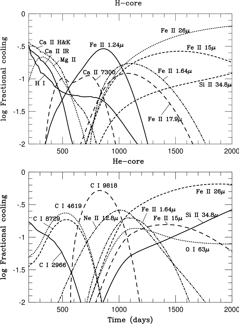
Figure 3: Fractional cooling by the most important transitions in the H-core zone and the He-core zone, as a function of time.

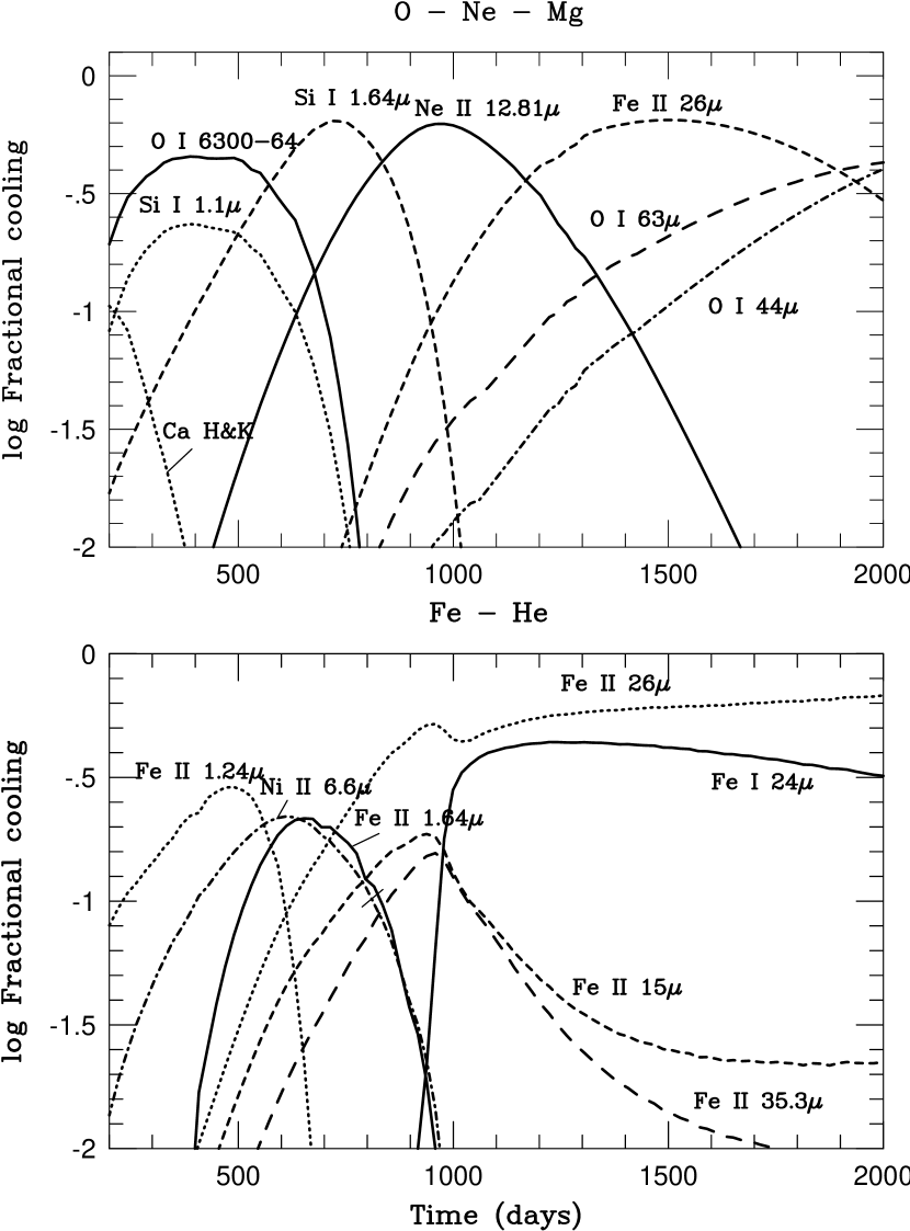
Figure 4: Fractional cooling in the O – Ne – Mg and the Fe – He zones, as a function of time.

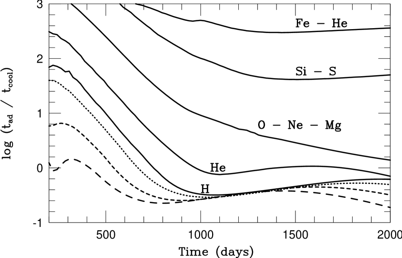
Figure 5: Ratio of adiabatic to radiative cooling. The hydrogen curves are from the top the hydrogen in the core (solid), and the hydrogen envelope at 2000 $\rm~{}km~{}s^{-1}$ (dotted), 2800 $\rm~{}km~{}s^{-1}$ (short dashed) and 4100 $\rm~{}km~{}s^{-1}$ (long dashed), respectively.

Because the contribution from the different zones to a given line reflects the temperature of this zone, we now comment on the detailed evolution of each of these zones. To guide in this discussion we show in Figures 3 and 4 the contributions to the fractional cooling from some of the most important transitions in the H-core, the He-core, the O – Si – S, and the Fe – He zones. Note that these figures give the collisional cooling of the gas (see equation 3), which is in general not the same as the radiative losses. In particular, transitions which are completely radiatively forbidden may be strong collisional coolants. An example is the $a{}^{6}D_{5/2}-a{}^{6}D_{9/2}~{}\lambda~{}14.98~{}\mu$m transition in the ground multiplet of Fe II, which contributes a comparable amount to the cooling as the observationally important $a{}^{6}D_{7/2}-a{}^{6}D_{9/2}~{}\lambda~{}25.99~{}\mu$m transition. The excitations in the $~{}\lambda~{}14.98~{}\mu$m transition mainly decay by emitting line emission at $~{}\lambda~{}25.99\mu$m and $~{}\lambda~{}35.35\mu$m. We also show in Figure 5 the relative importance of adiabatic cooling.

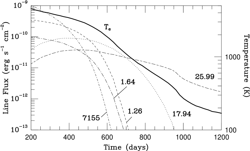
Figure 6: The strongest Fe II lines from the iron core, together with the temperature in the same region. Note the gradual transition from optical to near-IR, to far-IR lines, as the IR-catastrophe sets in at $\sim 600$ days.

In the Fe – He rich shells heating is dominated by non-thermal heating of the free electrons at all times. A large fraction of this is due to the deposition of positrons. At 200 days this is $\sim$ 45 % of the non-thermal heating, while at 1500 days the corresponding number is $\sim$ 97 %. At most 20 % (but most of the time less than 10 %) of the heating is due to photoionization. The cooling is at all times dominated by line cooling from Fe II. The IR-catastrophe sets in at $\sim 500$ days, when the temperature is $2700$ K, and is directly reflected in the relative fluxes from the iron core (Fig. 6). As the temperature falls, there is a gradual progression of cooling from UV, to optical lines like $~{}\lambda~{}7155$, to near-IR, e.g., $~{}\lambda~{}\lambda~{}$ 1.26, 1.64 $\mu$m, to far-IR fine structure lines. At $t\gtrsim 500$ days, Fe II $~{}\lambda~{}\lambda~{}$ 17.94, 25.99 $\mu$m are the most important, and finally, at $t\gtrsim 750$ days, only the $~{}\lambda~{}$ 25.99 $\mu$m line contributes to the cooling. Once the IR-catastrophe has occurred, the temperature is nearly constant at $\sim 140$ K. Because of the efficient fine-structure cooling, adiabatic cooling is not important before 2000 days.

From the observations of the [Fe II] $~{}\lambda~{}$ 25.99 $\mu$m line we can get an observational estimate of the temperature in the iron region, assuming that the $~{}\lambda~{}$ 25.99 $\mu$m line is the dominant coolant. This only applies to the iron-rich gas and not to e.g. the hydrogen- or helium-rich components. In the iron-rich gas the optical depth of the $~{}\lambda~{}25.99\mu$m line is

$$\tau_{26\mu} = 28.5~{}f_{\rm Fe}^{-1}~{}\left({M_{\rm Fe}\over 0.07~{}{~{}\rm M}_{\odot}}\right)~{}\left({V\over 2000~{}\rm~{}km~{}s^{-1}}\right)^{-3}~{}$$ (67)

$$\left({t\over 500~{}{\rm days}}\right)^{-2}~{}(1-e^{-554{\rm~{}K}/T}).$$

With a filling factor $f_{\rm Fe}\approx 0.5$ (Li, McCray & Sunyaev 1993), and a temperature $\gtrsim 200$ K (Fig. 2), the $~{}\lambda~{}$ 25.99 $\mu$m line is likely to be thick to at least $\sim 2000$ days. The critical density of the $~{}\lambda~{}$ 25.99 $\mu$m line is $\sim 2\times 10^{4}{\rm~{}cm^{-3}}$, so the a⁶D_9/2 and a⁶D_7/2 levels should be in LTE, and therefore radiate at the blackbody rate,

$${dE\over dtdV} = {8\pi hc\over\lambda^{4}~{}t~{}(e^{hc/\lambda kT}-1)}$$ (68)

$$= 2.55\times 10^{-12}~{}(e^{554{\rm~{}K}/T}-1)^{-1}~{}$$ (70)

$$\left({t\over 500~{}{\rm days}}\right)^{-1}{\rm~{}erg~{}s^{-1}~{}{\rm cm^{-3}}}.$$

(e.g., Fransson 1994). The heating rate in the iron-rich gas is

$${dE\over dtdV} = {\epsilon_{\rm H}~{}D_{\gamma}~{}\rho\over 4\pi R^{2}_{\rm core}}(\kappa_{\gamma,56}~{}L_{\gamma,56}+\kappa_{\gamma,57}~{}L_{\gamma,57})$$ (71)

$$\approx 0.75\times 10^{-9}~{}f_{\rm Fe}^{-1}~{}D_{\gamma}~{}\left({M_{\rm Fe}\over 0.07~{}{~{}\rm M}_{\odot}}\right)^{2}~{}$$

$$\left({V_{\rm core}\over 2000~{}\rm~{}km~{}s^{-1}}\right)^{-5}~{}\left({t\over 500~{}{\rm days}}\right)^{-5}~{}$$

$$e^{-t/111.3{}^{d}}~{}(1+1.2\times 10^{-3}~{}e^{t/155.6{}^{d}})~{}{\rm~{}erg~{}s^{-1}~{}{\rm cm^{-3}}}.$$

We have taken a fraction $\epsilon_{\rm H}\approx 0.5$ going into heating (KF92), and assumed a ⁵⁷Co mass of $3.3\times 10^{-3}{~{}\rm M}_{\odot}$. At $t\gtrsim 900$ days the $~{}\lambda~{}25.99~{}\mu$m line dominates the cooling (Fig. 6), and we can estimate the temperature in the gas by balancing the two expressions above. Setting $D_{\gamma}\approx 2.5$ (KF92) we obtain

$$T_{e} \approx 554~{}\{\ln[1+1.4\times 10^{-3}\left({M_{\rm Fe}\over 0.07~{}{~{}\rm M}_{\odot}}\right)^{-2}~{}f_{\rm Fe}~{}$$ (76)

$$\left({V_{\rm core}\over 2000~{}\rm~{}km~{}s^{-1}}\right)^{5}~{}\left({t\over 500~{}{\rm days}}\right)^{4}~{}$$

$${e^{t/111.3{}^{d}}\over(1+1.2\times 10^{-3}~{}e^{t/155.6{}^{d}})}]\}^{-1}~{}{\rm K}.$$

At 900 days we find for $f_{\rm Fe}=0.5$ that $T_{e}\approx 191$ K, at 1000 days $T_{e}\approx 140$ K, at 1200 days $T_{e}\approx 97$ K, and at 1500 days $T_{e}\approx 73$ K. These temperatures are about a factor of two less than those in Figure 2. In spite of this, equation (76) provides a good illustration of the sensitivity of the temperature to the parameters involved. It also reproduces the leveling off of the temperature in the Fe – He core at $t\gtrsim 1000$ days (Fig. 2).

The total luminosity in the $~{}\lambda~{}25.99~{}\mu$m line from the Fe – He core is

$$L_{26\mu} = {32\pi^{2}~{}h~{}c~{}f_{\rm Fe}V_{\rm core}^{3}~{}t^{2}\over 3\lambda^{4}~{}(e^{hc/\lambda kT}-1)}$$ (77)

$$= 6.9\times 10^{36}f_{\rm Fe}~{}\left({V_{\rm core}\over 2000~{}\rm~{}km~{}s^{-1}}\right)^{3}~{}$$

$$~{}\left({t\over 500~{}{\rm days}}\right)^{2}~{}(e^{554{\rm~{}K}/T}-1)^{-1}\rm~{}erg~{}s^{-1}.$$

The observed luminosity at 636 days was $\sim 6.0\times 10^{36}\rm~{}erg~{}s^{-1}$ (Colgan et al. 1994). Multiplying this by a factor 1.7 to account for dust absorption, and assuming $f_{\rm Fe}\approx 0.5$ gives a temperature of $1270$ K at this epoch. However, in Paper II we will show that there is likely to be a considerable contribution to the flux of the $~{}\lambda~{}$ 25.99 $\mu$m line from the hydrogen component. This temperature should therefore be considered as an upper limit. In our numerical model we find $T_{e}\approx 1520$ K at 636 days. Given the uncertainties in the filling factor and the dust absorption this is probably consistent with this temperature.

The temperature in the iron zone has also been calculated by Li, McCray & Sunyaev (1993). In their calculations they consider clumps consisting of only iron, cobalt, and nickel. In nucleosynthesis models there is a significant fraction of helium ($\sim 50\%$ by number), microscopically mixed with the iron, as a result of the alpha-rich freeze-out. In our calculations we find that, even for X(He) $\approx 0.5-0.7$, helium has a negligible effect on the conditions in the iron core. The reason is that only $\sim$ 10 % of the energy is deposited in helium, and $\sim$ 90 % in the iron peak elements. The temperature we find agrees well with that found by Li & McCray.

In the Si – S shells the temperature evolution differs somewhat between the two models. The instability sets in earlier in the 11E1 model, at $\sim 800$ days, compared to $\sim 900$ days for the 10H model. The temperature at $t\gtrsim 1000$ days is higher by a factor of up to $\sim 1.4$ for the 11E1 model, because of a higher positron deposition in this model. Non-thermal heating dominates at all epochs, but photoionization of mainly Ca I, Si I, and S I  contribute up to as much as 40 % of the heating. The positron contribution to the non-thermal heating is 10 – 20 % at 200 days, and more than 70 – 90 % at 2000 days. Important coolants in these shells are Si I, S I, Ca II, Fe I – II, and Ni I – II.

Also in the O – Si – S shells in the 10H model and the O – Ne – Mg shells in the 11E1 model the temperature evolution differs somewhat. The instability sets in somewhat earlier in the 11E1 model, at $\sim$ 800 days compared to $\sim$ 1000 days for the 10H model. We find that the temperature is slightly lower in the O – Si – S zones in 10H, compared to that in the O – Ne – Mg zones of 11E1. At 2000 days the temperature is $\sim$ 100 K in both models.

Calculations of the temperature in the oxygen core, with and without CO, have been made by Liu & Dalgarno (1995). In their CO free case they find a temperature of $\sim$ 2200 K at 800 days, which is considerably higher than ours. The reason is likely to be found in the differences between our models in the composition and in the trace elements included. Li & McCray (1992) estimate the oxygen temperature from observations of the [O I] $~{}\lambda~{}\lambda~{}$ 6300, 6364 emission doublet to T $\approx$ 4100 K at 200 days, and T $\approx$ 2900 K at 500 days, in fair agreement with what we find.

The temperature within the O – C region decreases from $\sim$ 4000 – 5500 K at 200 days, to $\sim$ 2700 K at 600 days, to $\sim$ 1500 K at 1000 days, and to $\sim$ 110 K at 2000 days. However, the O – C zone is favorable to CO formation. Because we neglect the very efficient cooling by CO, our temperatures are probably over-estimated by a large factor. Liu & Dalgarno (1995) find that for the CO emitting regions the temperature is constant at $\sim$ 1800 K for the first year, after which it decreases to $\sim$ 700 K at 800 days. We will discuss the implications of this for the line emission in Paper II.

In both of the oxygen-rich zones the temperature decreases nearly adiabatically once the IR-catastrophe has occurred, in contrast to the Fe – He region (Fig. 5). The IR-catastrophe occurs slightly earlier in the O – Si – S / O – Ne – Mg regions compared to the O – C region. However, inclusion of CO-cooling will affect this result.

For the helium shells within the core, line cooling is of the same order as adiabatic cooling after $\sim$ 1000 days, resulting in a faster decline in the temperature than the adiabatic $T\propto t^{-2}$ cooling. Outside of the core, adiabatic cooling becomes important at a somewhat earlier time at $\sim$ 800 days.

In the hydrogen shells within the core, adiabatic cooling dominates line cooling after $\sim$ 800 days (Fig. 5). Figure 7 shows the temperatures for the different shells in the hydrogen envelope. The envelope density is in this, and in all other models, given by equation (64), unless otherwise stated. The temperature in the envelope is at first constant, or even decreasing, up to $\sim$ 250 days. This decrease is sensitive to the exact gamma-ray transfer, and therefore model dependent. After $\sim$ 250 days the temperature decreases nearly adiabatically, with the highest temperature closest to the core. Adiabaticity sets in first in the high velocity regions with the lowest density.

3.2 Ionization

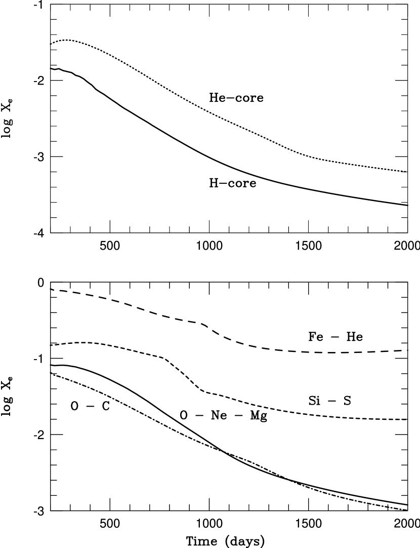
Figure 8: The evolution of the electron fraction for representative shells for the different composition zones in the core for the 11E1 model.

In Figure 8 we show the evolution of the ionization for the same shells in the 11E1 model for which we previously showed the temperature and cooling. The most interesting results are the gradual increase in the ionization as we go to more and more advanced burning stages. This is mainly a result of the decrease in the number of ions for constant density as we go to the heavier elements. Later than $\sim 1000$ days the ionization in the iron core becomes nearly constant with time, in contrast to the oxygen-rich zones.

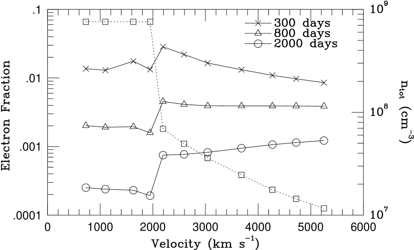
Figure 9: Electron fraction as a function of velocity for the hydrogen-rich regions at three different epochs. At 300 days steady state is a good assumption, at 800 days the freeze-out effects start to become important. Freeze-out effects are more pronounced in the outer envelope region (V $\geq 2000\rm~{}km~{}s^{-1}$) where the density is lower. Also shown, as the dotted curve, is the number density for the hydrogen-rich regions at 800 days.

Freeze-out of the ionization was discussed in connection to the bolometric light curve in Fransson & Kozma (1993). Because of the decreasing density the recombination time scale may become longer than the radioactive decay time scale. The evolution of the ionization differs between the different composition regions. The freeze-out effects sets in for all compositions at $\sim 800-900$ days. However, the degree of freeze-out differs between the composition zones, and to a larger extent, between the core and the envelope regions. The ratio of emitted energy, $L_{\rm em}$, to deposited energy, $L_{\rm dep}$, is a useful measure of the degree of freeze-out in the different regions (Fransson & Kozma 1993). Within the metal-rich regions in the core $L_{\rm em}/L_{\rm dep}\sim 1.5$ is reached. The corresponding number for the hydrogen-rich regions within the core is $\sim 1.6-2.0$. In the envelope, freeze-out sets in somewhat earlier (around 750 days for the regions furthest out) and a maximum of $L_{\rm em}/L_{\rm dep}\sim 2.5$ is reached. To see the effect of the freeze-out on the ionization we show in Figure 9 the electron fraction, $x_{e}$, as a function of velocity for the hydrogen-rich shells at three epochs, 300, 800 and 2000 days. The lower ionization at V $\lesssim$ 2000 $\rm~{}km~{}s^{-1}$ is caused by the higher density assumed in the core region, compared to the envelope (dotted line in Fig. 9). Because of the lower density, freeze-out effects are increasingly pronounced in the outer regions of the envelope. This is illustrated by the fact that the decrease in ionization is smaller in these regions than in the inner region of the envelope and within the core.

At 1000 days, the electron fraction and temperature in the envelope are both a factor of $2-4$ higher in the time-dependent case, compared to steady state. In the core, the increase in temperature and electron fraction is $\lesssim 1.4$ for the hydrogen and helium regions, while the difference in the metal-rich regions is small.

4 EFFECTS OF UV-FIELD AND CHARGE TRANSFER

The UV-radiation field determines the ionization balance especially of ions with low ionization potentials and with small abundances, like Na I, Mg I, Si I and Fe I. Our model probably gives a good representation of the emissivity in the different lines and continua. As has been discussed by several authors (e.g., Xu & McCray 1991, Fransson 1994, Li & McCray 1996), this radiation is severely affected by scattering by the many metal resonance lines present. In addition, in the hydrogen-rich regions scattering by H₂ may be important (Culhane & McCray 1995). The inclusion of these effects is beyond the scope of this paper. In Paper II we comment on their importance.

Besides the UV-field, charge transfer reactions are probably the most uncertain point in our calculations. Reaction rates involving hydrogen and helium are reasonably well known, because of their importance in the interstellar medium. Reactions between metals are in most cases uncertain, and in many cases completely unknown. In the cases where rates are available these are usually motivated by their importance in atmospheric physics. Unfortunately, extrapolations from ions with similar atomic structure are usually impossible. In some cases one can make an educated guess whether a certain reaction will be fast, if a near resonance between the energy levels of the different ions is present. This is e.g. the case for O II + Ca I $\rightarrow$ O I + Ca II, where the $5p{}^{2}P_{1/2}$ level in Ca II has an energy which together with the ionization potential of Ca I is nearly equal to the O I ionization potential. Consequently, the reaction rate is high, $3.8\times 10^{-9}(T_{e}/10^{3}{~{}\rm K})^{1/2}{~{}\rm cm^{3}~{}s^{-1}}$ (Rutherford & Vroom 1972). There are also cases where this rule of thumb fails, and it is therefore of interest to estimate the influence of these uncertainties for our calculations.

An illustration of the sensitivity to charge transfer can be obtained by a simple model with only two elements. Of particular interest for the discussion of the O I recombination lines in Paper II is charge transfer of Si I and O II in the O – Si – S component. The Si I + O II $\rightarrow$ Si II + O I reaction can, like the O II + Ca I reaction, be expected to be fairly rapid, based on the near resonance with the $3p{}^{4}P$ state in Si II, with an energy difference of only 0.12 eV from the difference in ionization potentials of O I and Si I. Each charge transfer reaction will then give rise to a photon in the Si II] $~{}\lambda~{}\lambda~{}2334-2350$ multiplet, contributing to the UV-field.

In steady state the ionization balance is determined by (see eq. [12])

$$\Gamma_{{\rm OI}}n_{{\rm OI}} = n_{\rm SiI}n_{\rm OII}\xi^{\rm CT}_{\rm OII+SiI}+\alpha_{\rm OII}n_{e}n_{\rm OII}$$ (79)

$$(\Gamma_{{\rm SiI}}+n_{\rm OII}\xi^{\rm CT}_{\rm OII+SiI})n_{{\rm SiI}} = \alpha_{\rm SiII}n_{e}n_{\rm SiII}.$$ (80)

where $\Gamma_{{\rm OI}}$ is the non-thermal ionization rate of O I, and similarly for Si I (eq. [32]). In addition, we have the number and charge conservation equations

$$n_{\rm OI}+n_{\rm OII} = n_{\rm O}$$ (81)

$$n_{\rm SiI}+n_{\rm SiII} = n_{\rm Si}$$ (82)

$$n_{\rm SiII}+n_{\rm OII} = n_{e}$$ (83)

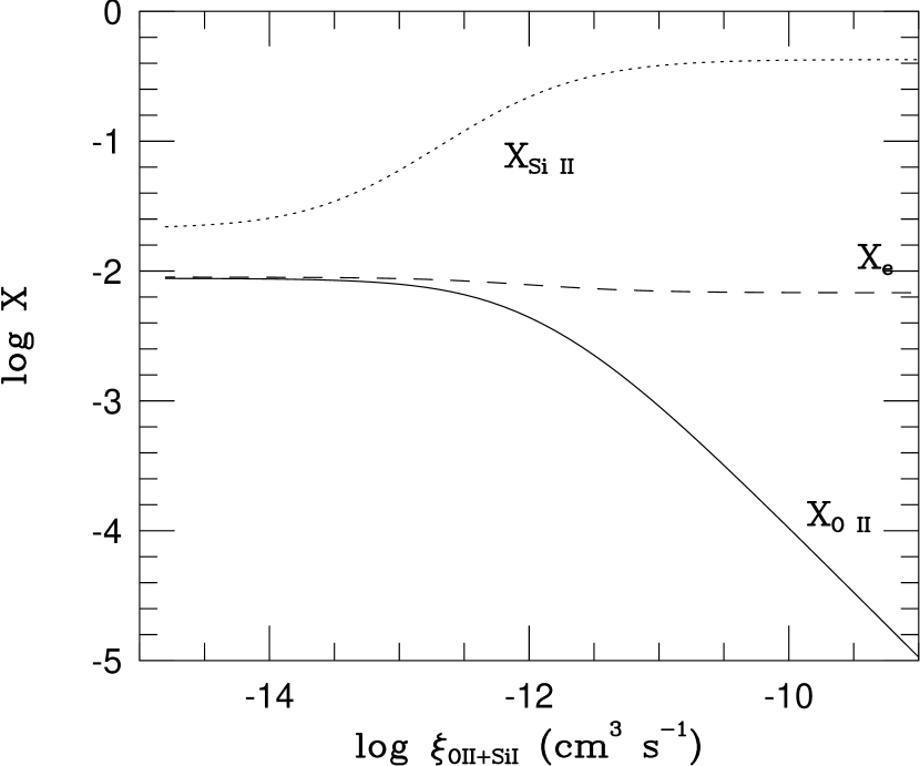
Figure 10: Electron and ionic fractions of O II and Si II, as a function of the Si I + O II $\rightarrow$ Si II + O I charge transfer rate.

These equations can easily be solved for a given epoch, and in Figure 10 we show the ionic abundances at 800 days for the case $X({\rm Si})=1.6\times 10^{-2}$ and $X({\rm O})=0.98$ as a function of the charge transfer rate between Si I + O II. These abundances are similar to the 11E1 O – Ne – Mg region. Although the total electron fraction only varies by $\sim 25$ % over the range $\xi^{\rm CT}_{\rm OII+SiI}=10^{-15}-10^{-8}{~{}\rm cm^{3}~{}s^{-1}}$, the individual states of ionization vary considerably. For $\xi^{\rm CT}_{\rm OII+SiI}\gtrsim 10^{-11}{~{}\rm cm^{3}~{}s^{-1}}$, basically all O II has disappeared, while the fraction of Si II increases. This behavior is easy to understand, since when $\xi^{\rm CT}_{\rm OII+SiI}~{}n_{\rm SiI}/\alpha_{\rm OII}~{}n_{e}\gtrsim 1$ the O II fraction decreases proportional to this ratio. The fraction of Si II increases correspondingly. The total electron fraction changes by a factor $\alpha_{\rm OII}/\alpha_{\rm SiII}$. In this case $\alpha_{\rm OII}/\alpha_{\rm SiII}\sim 1$, and only a minor change occurs. If $n_{\rm Si}\lesssim n_{e}$ the neutral fraction of silicon will decrease substantially. If instead $n_{\rm Si}\gg n_{e}$, only a minor change in the fraction of Si I will occur. This illustrates a general characteristic of charge transfer. Only the minor constituents, including ions of abundant elements, of a given zone are affected be this process, in this case O II, Si I and Si II, but not O I. This agrees with the result of Swartz (1994), where he finds that if the helium abundance is larger than the metal abundance the charge transfer reactions do not greatly affect the ionization balance and level populations of helium.

We have tested this simple model by assuming an O II + Si I charge transfer rate of $10^{-9}{~{}\rm cm^{3}s^{-1}}$ in our full code. This leads to a large decrease of the O II fraction, as expected. There is, however, little change in the Si I or Si II fractions. The reason for this is that another charge transfer reaction, Mg I + Si II $\rightarrow$ Mg II + Si I has a large rate. Therefore, Si II only acts as a mediator of the charge transfer from O II to Mg II. This illustrates the gradual transfer of the ionization to the low ionization potential elements, as well as the general importance of charge transfer for the low abundance ions (including ionized states of abundant elements, e.g. O II).

5 DUST COOLING

The presence of dust in SN 1987A can have important consequences for the line emission. Besides the effect of absorption, which will be discussed in Paper II, dust cooling may also influence the thermal evolution of the regions where dust has formed. Although a self-consistent discussion of this involves a solution of the equations describing the nucleation, which is beyond the scope of this paper, we can see the qualitative effects of the dust by a simple model, relying on previous studies of the dust formation in SN 1987A by Kozasa, Hasegawa & Nomoto (1989, 1991).

Kozasa et al. show that the most likely monomers to form are corundum, ${\rm Al}_{2}~{}{\rm O}_{3}$, and enstatit, ${\rm Mg}~{}{\rm Si}~{}{\rm O}_{3}$. ${\rm Al}_{2}~{}{\rm O}_{3}$ forms first at a temperature of $\sim 1600$ K, while ${\rm Mg}~{}{\rm Si}~{}{\rm O}_{3}$ forms at a somewhat lower temperature, $\sim 1500$ K. While Kozasa et al. mainly considered microscopically mixed cases, we think this is unlikely, as already argued. Therefore, there is little overlap of regions with a substantial abundance of iron and oxygen, and the formation of ${\rm Fe}_{3}~{}{\rm O}_{4}$ is likely to be inefficient. Here we consider mainly the formation of ${\rm Al}_{2}~{}{\rm O}_{3}$ and ${\rm Mg}~{}{\rm Si}~{}{\rm O}_{3}$ in the O – Ne – Mg zone, where both magnesium, silicon, and aluminum are abundant, together with oxygen.

To model the formation of these grains we simply assume that they form at the condensation temperatures above. Kozasa et al. (1991) find a radius for the ${\rm Al}_{2}~{}{\rm O}_{3}$ grains of $\sim 10$ Å, while the ${\rm Mg}~{}{\rm Si}~{}{\rm O}_{3}$ grains have a radius of $\sim 70$ Å. The cooling rate per dust grain is, assuming that $T_{\rm dust}\ll T_{e}$, (Dwek & Arendt 1992)

$$\Lambda_{\rm dust}=1.26\times 10^{-27}~{}[{n\over A_{\rm mean}^{1/2}}+({m_{p}\over m_{e}})^{1/2}~{}n_{e}]~{}a^{2}~{}T_{e}^{3/2}\rm~{}erg~{}s^{-1},$$ (84)

where $a$ is the grain radius in Å. The first term represents cooling by atoms and the second that by the free electrons.

The total amount of dust formed is uncertain. Here we assume, consistent with Kozasa et al. , that all aluminum in the O – Ne – Mg zone goes into ${\rm Al}_{2}~{}{\rm O}_{3}$ and all silicon into ${\rm Mg}~{}{\rm Si}~{}{\rm O}_{3}$ grains. In the 11E1 model, $X({\rm Mg})\approx 7.1\times 10^{-2}$, and $X({\rm Si})\approx 1.6\times 10^{-2}$. We take the aluminum abundance from the 11E1 model to be $8.3\times 10^{-3}$ by mass. The total mass of the O – Ne – Mg zone is $1.8{~{}\rm M}_{\odot}$, giving $M({\rm Al})=1.5\times 10^{-2}{~{}\rm M}_{\odot}$, and the mass of ${\rm Al}_{2}~{}{\rm O}_{3}$ is then $2.8\times 10^{-2}{~{}\rm M}_{\odot}$ and the mass of ${\rm Mg}~{}{\rm Si}~{}{\rm O}_{3}\sim 0.17{~{}\rm M}_{\odot}$. With a size of $1.7~{}$Å  and $2.06~{}$Å  per key species (Kozasa et al. 1989), the total number of grains in the two cases are therefore $1.8\times 10^{51}~{}(M({\rm Al})/1.5\times 10^{-2}{~{}\rm M}_{\odot})~{}(a/10{\rm~{}\AA})^{-3}$ and $5.2\times 10^{49}~{}(M({\rm Si})/5\times 10^{-2}{~{}\rm M}_{\odot})~{}(a/70{\rm~{}\AA})^{-3}$, respectively. The total, optically thin cooling rate for ${\rm Al}_{2}~{}{\rm O}_{3}$ is then

$$\Lambda_{\rm dust}^{0} = 1.1\times 10^{-13}~{}\left({M({\rm O})\over 2{~{}\rm M}_{\odot}}\right)~{}\left({M({\rm Al})\over 1.5\times 10^{-2}{~{}\rm M}_{\odot}}\right)~{}$$ (87)

$$\left({V_{\rm core}\over 2000\rm~{}km~{}s^{-1}}\right)^{-6}~{}\left({t\over 500{\rm~{}days}}\right)^{-6}~{}\left({f_{\rm O}\over 0.1}\right)^{-2}$$

$$~{}\left({a\over 10{\rm~{}\AA}}\right)^{-1}~{}(1+171~{}x_{e})~{}T_{e}^{3/2}\rm~{}erg~{}s^{-1}~{}cm^{-3},$$

and for ${\rm Mg}~{}{\rm Si}~{}{\rm O}_{3}$

$$\Lambda_{\rm dust}^{0} = 1.7\times 10^{-13}~{}\left({M({\rm O})\over 2{~{}\rm M}_{\odot}}\right)~{}\left({M({\rm Si})\over 5\times 10^{-2}{~{}\rm M}_{\odot}}\right)~{}$$ (91)

$$\left({V_{\rm core}\over 2000\rm~{}km~{}s^{-1}}\right)^{-6}~{}\left({t\over 500{\rm~{}days}}\right)^{-6}~{}\left({f_{\rm O}\over 0.1}\right)^{-2}$$

$$~{}\left({a\over 70{\rm~{}\AA}}\right)^{-1}~{}(1+171~{}x_{e})~{}T_{e}^{3/2}\rm~{}erg~{}s^{-1}~{}cm^{-3}.$$

As the temperature falls the cooling will eventually exceed the black-body limit, at which time the temperature stabilizes.

Assuming that dust formation occurs when the temperature has decreased to the condensation temperatures for the two species, the ${\rm Al}_{2}~{}{\rm O}_{3}$ formation takes place at $\sim 800$ days. At the time of dust formation in our model, immediately before the temperature drop, the ratio of the dust cooling and line cooling is $\sim 50$. Therefore, as soon as the dust forms it immediately cools the gas to a very low temperature, at which the optically thick dust cooling balances the heat input. Because of the dramatic cooling, the ${\rm Mg}~{}{\rm Si}~{}{\rm O}_{3}$ formation occurs at the same epoch.

A dust formation epoch at $\sim$ 800 days is later than the observations indicate. Possible reasons for this discrepancy could either be extra cooling in the oxygen-rich gas due to e.g. molecular cooling by SiO, or the simplified assumption of instantaneous dust formation at the temperatures above. Other possible, and perhaps the most likely, sites for dust formation are in the O – C zone and in the iron-rich core. In the O – C region CO cooling could decrease the temperature enough for graphite to form. This scenario requires that not all carbon is locked up into CO. This is supported by the calculations done by Liu & Dalgarno (1995). They find a CO mass of $(1-2)\times 10^{-3}{~{}\rm M}_{\odot}$, while the total carbon mass in the O – C zone is $(1-10)\times 10^{-2}{~{}\rm M}_{\odot}$. A second possible site is the iron core, where the temperature is $\lesssim 1500$ K at $\sim 600$ days. Clumping may further decrease the temperature and thus the dust condensation epoch. The dust formation is likely to occur at different epochs at different positions in the ejecta, explaining the observed gradual formation of the dust.

In the optically thick limit we can calculate the dust temperature by balancing the gamma-ray energy absorbed in the O – Ne – Mg zone by the dust cooling to obtain

$$T_{\rm dust} = 1770~{}\left({V_{\rm core}\over 2000\rm~{}km~{}s^{-1}}\right)^{-1/2}~{}\left({t\over 500{\rm~{}days}}\right)^{-1}$$ (96)

$$~{}\left({f_{\rm cov}\over 0.4}\right)^{-1/4}~{}\left({\Delta\tau_{\gamma,\rm O}(500{\rm~{}days})\over 0.23}\right)^{1/4}~{}$$

$$e^{-t/445{\rm~{}days}}\rm~{}K.$$

We have here scaled the gamma-ray optical depth of the O – Ne – Mg zone by the value in our models at 500 days (Table 3). At 600 days we obtain $T_{\rm dust}=380$ K, and at 800 days 183 K. These values are in reasonable agreement with those determined by Wooden et al. (1993) and Colgan et al. (1994).

Although certainly too simplified, this discussion is indicative of the importance of the additional cooling where dust is formed. The cooling rate we estimate above is directly proportional to the amount of dust assumed to be formed, as long as the gas is optically thin. Because of the nearly full conversion of the key elements into dust, this should probably be considered as an upper limit. A serious discussion of the dust cooling requires a more physical model of the dust nucleation, along the lines of Kozasa et al.

A consequence of this scenario is a depletion of the elements in the oxygen region involved in the dust condensation. This has little effect on oxygen. Both aluminum and silicon are by assumption completely depleted from the gas phase in this region, and magnesium is decreased by $\sim 20\%$ in the 11E1 model. Observational evidence for Si depletion, based on the [Si I] lines, has been prestented by Lucy et al. (1991). It is, however, not trivial to separate the effects of dust depletion and decrease in temperature on the strength of the Si emission.

6 CONCLUSIONS

The temperature and ionization of the supernova ejecta determine the evolution of the observed emission lines. In this paper we have made a considerable effort to calculate these as realistically as possible. Previous calculations have made various simplifications, which limit their applicability. Fransson & Chevalier (1987, 1989) neglected time-dependent effects, as well as the hydrogen-rich component. Li, McCray & Sunyaev (1993) and Liu & Dalgarno (1995) only considered the iron and oxygen-rich zones, respectively, and also neglected time-dependent effects. The only work comparable to ours is that by de Kool, Li & McCray (1997), which we became aware of only after this work was completed. In as far as we have been able to compare, we agree very well with their results in terms of both temperature and ionization. This comparison of completely independent calculations adds to the confidence of our results, within the assumptions of the model.

Except as input to the calculations of the line emission, our most important results concerns the IR-catastrophe at 600 – 1000 days in the metal zones. Other results of special interest concern adiabatic cooling later than 500 – 800 days in especially the hydrogen and helium regions, and the freeze-out of the ionization in the hydrogen envelope. Although some of these effects have been noted previously (Fransson & Chevalier 1987, 1989; Fransson & Kozma 1993), they are in this paper synthesized into a coherent picture. In Paper II we show how the temperature evolution is reflected in the line emission. In addition, both molecule and dust formation are sensitive to the temperature. In our models dust is formed too late in the O – Ne – Mg zones.

In spite of our effort to include physics as realistically as possible, there are still some major deficiencies, in particular our treatment of the UV-field, the neglect of molecular and dust cooling, and uncertainties in the charge transfer rates. Molecular cooling can have important consequences, as demonstrated by Liu & Dalgarno (1995), but is probably limited to the O - C zone, and the interface between the oxygen and silicon regions. As we will discuss in Paper II, the thermal line emission from the other regions would otherwise also be completely quenched. As our estimate of the dust cooling shows, a similar effect would occur where the dust forms. In this case, however, dust formation takes place where there is a strong drop in the temperature, because of the IR-catastrophe. The emission from the metal-rich zones is then dominated by non-thermal excitation, and the line emission is therefore insensitive to the temperature. These areas clearly deserve much further study.

Appendix A APPENDIX

A.1 Charge Transfer

Charge transfer reactions are important in determining the ionization balance for the trace elements. Unfortunately, rates are rather uncertain. The reactions we include in our calculations are given in Table A.2.7 together with references for the rates. Most charge transfer rates with hydrogen are from Kingdon & Ferland (1996), who give analytical fits to all the rates. This includes a compilation of both already available rates from different sources (see references therein), and newly calculated rates.

The data in Prasad & Huntress (1980) and Arnaud & Rothenflug (1985) are also compilations from various sources. The rates from Kimura, Lane, Dalgarno, & Dixson (1993) (H II + He I $\rightarrow$ H I + He II), and Kimura et al. 1993 (He II + C I $\rightarrow$ He I + C II) are low. For the reaction H II + Ca I $\rightarrow$ H I + Ca II we did not find any published data. As an estimate we use the same rate as for O II + Ca I $\rightarrow$ O I + Ca II.

Swartz (1994) estimates charge transfer reaction rates between helium and metals, using the Landau-Zener and modified Demkov approximations. He also estimates the rates for the charge transfer between excited states in He I ($2s^{1}S$, $2p^{1}P$, $2s^{3}S$, and $2p^{3}P$) and metals. The accuracy of these are probably not better than a factor of two to five. We therefore include the rates from Swartz separately, to examine their importance.

The rate for the Penning process, $7.5\times 10^{-10}(T/300K)^{1/2}{\rm cm^{3}s^{-1}}$, is from Bell (1970).

A.2 Model Atoms

A.2.1 H I

For H I we use a model atom consisting of 30 levels. For the 5 lowest $n$-states all $l$-states are included. The higher $n$-states, up to $n=20$, are treated as single levels.

We use expressions given by Brocklehurst (1971) for the transition probabilities between different $nl$-states ($A_{nl,n^{\prime}l^{\prime}}$). Only transitions with $\Delta l=\pm 1$ are assumed to have A-values greater than zero. The one exception is the two-photon transition, $2s-1s$, with a transition probability of $8.23~{}{\rm s^{-1}}$. When calculating transition probabilities between an upper $n$-state and a lower $nl$-states, as well as between two $n$-states, the following averages are used,

$$A_{n,n^{\prime}l^{\prime}}=\sum_{l=0}^{n-1}\frac{g_{l}}{g_{n}}A_{nl,n^{\prime}l^{\prime}},$$ (A1)

and

$$A_{n,n^{\prime}}=\sum_{l}\frac{g_{l}}{g_{n}}\sum_{l^{\prime}}A_{nl,n^{\prime}l^{\prime}}=\sum_{l^{\prime}}A_{n,n^{\prime}l^{\prime}}$$ (A2)

where $g_{l}=2(2l+1)$ is the statistical weight of the $l$-state, and $g_{n}=2n^{2}$ is the statistical weight of the $n$-state. In thermodynamic equilibrium, when the $l$-states are populated according to their statistical weights ($x_{nl}=x_{n}\frac{g_{l}}{g_{n}}$), we have

$$x_{n}A_{n,n^{\prime}l^{\prime}}=\sum_{l}x_{nl}A_{nl,n^{\prime}l^{\prime}}$$ (A3)

and

$$x_{n}A_{n,n^{\prime}}=\sum_{l,l^{\prime}}x_{nl}A_{nl,n^{\prime}l^{\prime}},$$ (A4)

motivating the expressions above.

Recombination coefficients to the $nl$-states are calculated using expressions in Brocklehurst (1971). The total recombination coefficient for hydrogen is given by Seaton (1959). These rates agree with the total recombination coefficients by Verner & Ferland (1996). In order to get the correct total recombination coefficient we increase the recombination coefficient to the highest ($n=20$) $n$-state, so that the sum of the recombination coefficients to all the levels equals the total recombination coefficient. This treatment is not correct for the highest levels, but should be a good approximation for the lower levels.

Collisions with both electrons and protons between $l$-states for a given $n$-level are included for the 5 lowest $n$-levels (Brocklehurst 1971, Pengelly & Seaton 1964). The total collisional excitation rates between different $n$-levels ($C_{nn^{\prime}}$) are from Johnson (1972). To divide the total rates into rates between different $l$-states we use the Bethe-approximation (Hummer & Storey 1987). For all $\Delta n>0$ and $\Delta l=\pm 1$ we use,

$$C_{nl,n^{\prime}l^{\prime}}=\frac{A_{nl,n^{\prime}l^{\prime}}}{A_{nn^{\prime}}}C_{nn^{\prime}}$$ (A5)

and

$$C_{n,n^{\prime}l^{\prime}}=\frac{A_{n,n^{\prime}l^{\prime}}}{A_{nn^{\prime}}}C_{nn^{\prime}}.$$ (A6)

This approximation gives,

$$x_{n}C_{n,n^{\prime}}=\sum_{l,l^{\prime}}x_{nl}C_{nl,n^{\prime}l^{\prime}},$$ (A7)

if the different $l$-states are assumed to be populated according to statistical weights.

Photoionization cross sections for individual $nl$-states, for $n>2$, are calculated using the expressions given by Brocklehurst (1971), and for the higher $n$-states by Seaton (1959). Photoionization cross sections for $n=1$ and $n=2$ are from Bethe & Salpeter (1957).

To solve the level populations for the hydrogen atom using the Sobolev approximation complications appear due to overlapping lines. Transitions between two $n$-states but different $l$-states have the same energy, and the lines may interact. However, because of the degeneracy this scattering is local, and the escape formalism may still be used. This case has been treated by Drake & Ulrich (1980), and we use their expressions.

The treatment of an $n$-state as a single level is correct for high enough densities, in which case the $l$-states become populated according to statistical weights. When calculating the line emission we recalculate the level populations for hydrogen using a 210 level atom containing all $l$-states up to $n=20$. This is done separately from the calculation of temperature and ionization, where we assume $l$-mixing for $n\geq 6$.

For the hydrogen two-photon continuum we use the two-photon distribution given by Nussbaumer & Schmutz (1984).

A.2.2 He I

We use a model atom for He I, consisting of 16 levels. The first 12 levels are $1s~{}^{1}S$, $2s~{}^{3}S$, $2s~{}^{1}S$, $2p~{}^{3}P$, $2p~{}^{1}P$, $3s~{}^{3}S$, $3p~{}^{3}P$, $3d~{}^{3}D$, $4s~{}^{3}S$, $4p~{}^{3}P$, $4d~{}^{3}D$, $4f~{}^{3}F$. The remaining 4 levels are fictitious levels, into which all the triplet levels up to $n=100$ have been combined. Collision strengths, and transition probabilities are from Almog & Netzer (1989). Verner & Ferland (1996) have calculated recombination coefficients, both total and to the different excited states, for the entire temperature range, 3 – $10^{9}$ K, which we use.

In our model we use the direct recombination coefficients calculated by Verner & Ferland (1996) to all levels except to $2s~{}^{1}S$ and $2p~{}^{1}P$ and the $4p~{}^{3}P$ and $4f~{}^{3}F$ states. The reason for this is that the $2s~{}^{1}S$ and $2p~{}^{1}P$ states are the only excited singlet levels included in the model atom by Almog & Netzer (1989). Including only direct recombinations to these would therefore under-estimate the total recombination rate, including higher states. We use the fit given by Almog & Netzer, which is, however, uncertain at low temperatures. This fact introduces some uncertainty in the He I two-photon continuum at low temperatures.

For the $4p~{}^{3}P$ and $4f~{}^{3}F$ levels we use rates from Almog & Netzer data in the temperature interval 10000 to 20000 K, extrapolating this to lower temperatures by $\alpha\propto T^{-0.5}$. This is in agreement with the temperature dependence Bates (1990) finds for low temperatures. Recombination coefficients to the four highest, fictious levels are from Almog & Netzer in the temperature interval 10000 – 20000 K. The temperature dependence is corrected for lower temperatures, using $\alpha\propto T^{-0.5}$ for $T<$ 1000 K. The rates of these four highest recombination coefficients were normalized to achieve the correct total recombination coefficient.

For the ground state photoionization cross sections are from Verner et al. (1996), while the excited state cross sections are from Koester et al. (1985). For the helium two-photon continuum, between the 2s ¹S and the 1s ¹S states, we use the distribution given by Drake, Victor, & Dalgarno (1969).

In the Spencer-Fano calculations we include non-thermal excitations to the following excited levels: $2s~{}^{3}S$, $2s~{}^{1}S$, $2p~{}^{3}P$, $2p~{}^{1}P$, $3s~{}^{3}S$, $3p~{}^{3}P$, $3d~{}^{3}D$. References for the cross sections are given in KF92.

A.2.3 O I

Our O I  atom consists of 13 levels, $2p^{4}~{}^{3}P_{2}$, $2p^{4}~{}^{3}P_{1}$, $2p^{4}~{}^{3}P_{0}$, $2p^{4}~{}^{1}D$, $2p^{4}~{}^{1}S$, $3s~{}^{5}S_{o}$, $3s~{}^{3}S_{o}$, $3p~{}^{5}P_{o}$, $3p~{}^{3}P_{o}$, $4s~{}^{5}S_{o}$, $4s~{}^{3}S_{o}$, $3d~{}^{5}D_{o}$, $3d~{}^{3}D_{o}$. Transition probabilites and collision strengths are from Bhatia & Kastner (1995). We include non-thermal excitations from the ground state to all excited levels. References for the cross sections used are given in KF92. For the fine structure transitions within the ${}^{3}P$ state A-values and collision strengths for O I are from Berrington (1987).

The total radiative recombination coefficient is from Chung, Lin, & Lee (1991). Recombination coefficients to the individual levels are from Julienne, Davies & Oran (1974), renormalized by a factor 1.38 to give a total rate equal to that of Chung et al.

Photoionization cross sections are from Verner et al. (1996) for the ground state. For the excited states the data are from Dawies & Lewis (1973).

A.2.4 Ca II

The six-level model atom for Ca II  consists of the $4s~{}^{2}S$, $3d~{}^{2}D$, $4p~{}^{2}P$, and $5s~{}^{2}S$ levels. A-values are from Ali & Kim (1988), Zeippen (1990), and Wiese et al. (1969). Collision strengths are from Burgess et al. (1995), except between the sublevels of 3d, which are from Shine (1973). Ground state photoioinization cross sections are from Verner et al. (1996). For the excited states data are from Shine (1973), while recombination rates are from Shull & Van Steenberg (1982).

A.2.5 Fe I-IV

Fe I-IV are treated as multilevel atoms with 121 levels for Fe I, 191 levels for Fe II, 110 levels for Fe III, and 43 levels for Fe IV. A-values for Fe I  are from Kurucz & Peytremann (1975) and from Axelrod (1980), and collision strengths from Axelrod (1980). The accuracy of the latter are probably low. For Fe II, A-values and collision strengths are from the Iron Project (Nahar 1995, Zhang & Pradhan 1995), and from Garstang (1962). Additional A-values are from Kurucz (1981). For Fe III  and Fe IV  data come from Garstang (1957) and Kurucz & Peytremann (1975), Berrington et al. (1991). Total recombination rates are from Shull & Van Steenberg (1982), and the fractions of the radiative recombination going to the ground state are from Woods, Shull, & Sarazin (1981).

For Fe I  and Fe II  the total photoionization cross sections are from Verner et al. (1996). Only photoionizations from the first five levels (i.e., the ground multiplet) are included for Fe I  and Fe II. The same cross section is assumed for all levels in the ground multiplet.

It is highly time consuming to calculate the level populations for the large Fe I-IV ions. In order to speed up the calculations we reduce the number of levels in these, if possible. The first time steps of the calculation always use ’full’ iron-atoms. At later epochs, the populations of the ’full’ atoms are calculated every few days. The highest levels, which in these calculations together contribute less than 0.1 % of the total emission or cooling/heating, are then excluded in the following time steps. The error in the total emission introduced by this procedure is therefore never larger than $\sim 0.1\%$.

A.2.6 Ni I-II and Co II

We include Ni I, Ni II, and Co II with a small number of levels in order to model the [Ni I] $~{}\lambda~{}$ 3.119 $\mu$m, [Ni I] $~{}\lambda~{}$ 7.505 $\mu$m, [Ni II] $~{}\lambda~{}$ 6.634 $\mu$m, [Ni II] $~{}\lambda~{}$ 10.68 $\mu$m, and the [Co II] $~{}\lambda~{}$ 10.52 $\mu$m lines. We assume that the ionization balances for cobolt and nickel are coupled to the ionization balance of iron by charge transfer (Li, McCray, & Sunyaev 1993). Due to lack of good atomic data we do not include non-thermal excitations or recombinations in calculating the line emission. Therefore, lines arising from these atoms are due only to thermal, collisional excitations by electrons.

Our Ni I atom has seven levels, consisting of the three lowest multiplets, $a^{3}F$, $a^{3}D$, and $a^{1}D$. Transition probabilities between levels within the $a^{3}F$ and the $a^{3}D$ multiplets are from Nussbaumer & Storey (1988), and transition probabilities between $a^{1}D$ and $a^{3}D$ from Garstang (1964).

The model atom for Ni II has eight levels, consisting of the three lowest terms, ${}^{2}D$, ${}^{4}F$, and ${}^{2}F$. Transition probabilities are from Nussbaumer & Storey (1982), and collision strengths are from Bautista & Pradhan (1996). For Co II we only include the lowest multiplet, $a^{3}F$, consisting of three levels, with transition probabilities from Nussbaumer & Storey (1988).

Unfortunately, no collision strengths are available for Ni I and Co II. Axelrod (1980) estimated collision strenths from the empirical relation

$$\Omega_{i,j}=Cg_{i}g_{j}$$ (A8)

where $g_{i}$, and $g_{j}$ are the statistical weights for the levels and $C$ is a constant. The constant was determined by a comparison with calculations by Garstang, Robb & Rountree (1978) for Fe III, and found to be $C=4\times 10^{-3}$ for transitions with $\lambda<10~{}\mu$m. For infrared transitions with $\lambda>10~{}\mu$m he adopted a higher value of the constant, $C=2\times 10^{-2}$. For the lowest 16 levels in Fe II we have checked this relation with the new Opacity Project collision strengths (Zhang & Pradhan 1995), and found $C=0.046$. In order to test equation (A8), we calculated collision strengths for Ni II using both $C=4\times 10^{-3}$, and $C=0.046$, and compared to the collision strengths from Nussbaumer & Storey (1982). The Ni II data are best reproduced by the constant from Axelrod, while our larger $C$ gives a factor of 10 too large collision strengths. Therefore the constant from Axelrod gives acceptable values for Ni II, while it under-estimates the collision strengths for Fe II by a factor of 10.

Li, McCray, & Sunyaev (1993) proposed an empirical formula for the collision strengths, based on known transitions in Fe II. In their formula the collision strength depends on the transition probability, and the energy difference between the levels, as well as on the statistical weight of the upper level. We do not find any clear correlation between transition probabilities, energy differences and collision strengths.

Given the result of the tests above, we feel that it is not possible to estimate the unknown collision strengths empirically to any degree of certainty. We therefore simply put the unknown collision strengths equal to 0.1 and await new atomic data.

A.2.7 Other Ions

References for the collisional ionization cross sections used for calculating the non-thermal ionization rates, are given in KF92. For the photoionization cross sections we use the analytical fits given by Verner et al. (1996).

Verner & Ferland (1996) give analytical fits to the radiative recombination coefficients in the temperature interval 3 K to $10^{9}$ K for recombinations towards H-, He-, Li- and Na-like ions. We use their data for recombination of He III, Mg III, and Na II. Radiative recombination coefficients from Gould (1978), and low-temperature dielectronic recombination coefficients from Nussbaumer & Storey (1983, 1986) are used for recombination of C II, C III, N II, O III, Mg II, Si II, Si III. We use rates from Shull & Van Steenberg (1982) for the Ne II, Mg II, S III, Ar II, Ca II recombinations. For S II we take radiative recombination rates from Gould (1978).

To calculate the cooling and line emission, the level populations for a number of model atoms are calculated, in steady state. C I, N II, O III, and S III are treated as six-level atoms, and C II, N I, O II, Si II, S I and S II as five-level atoms. References for the atomic data used in these model atoms are given in Lundqvist & Fransson (1996). In addition, for O II  we include non-thermal ionization of O I  to the excited $2p^{3}~{}^{2}D^{o}$ and $2p^{3}~{}^{2}P^{o}$ levels in O II (KF92).

The following transitions are calculated in the two-level approximation : ${\rm C\,II}~{}\lambda~{}1334$, $[{\rm Ne\,II}]~{}\lambda~{}12.814~{}\mu$m, ${\rm Na\,I}~{}\lambda~{}2843$, ${\rm Mg\,I}]~{}\lambda~{}4571$. A-values and collision strengths are from Mendoza (1983), Fabrikant (1974), Hayes & Nussbaumer (1984), Nussbaumer & Storey (1986), and Morton (1991).

For Si I  we include the $3p^{2}~{}^{3}P$, $3p^{2}~{}^{1}D$, and $3p^{2}~{}^{1}S$ levels, plus the fine structure transitions of the ${}^{3}P$ ground state. A-values are from Mendoza (1983), and collision strengths for $3p^{2}~{}^{3}P$ to $3p^{2}~{}^{1}D$ from Pindzola, Bhatia, & Temkin (1977). For the other transitions we estimate collision strengths from C I  and O I.

For ${\rm Na\,I}~{}\lambda~{}2843$, ${\rm Mg\,I}~{}\lambda~{}2852$, and ${\rm Mg\,II}~{}\lambda~{}\lambda~{}2795,2802$ we include non-thermal excitation with cross sections given in KF92. The cross section for ${\rm Mg\,I}]~{}\lambda~{}4571$ is from Fabrikant (1974).

Lines arising as a result of radiative recombination can be strong for abundant elements, unless charge transfer is more efficient. An important example is recombination to Mg I, where the strongest line is expected to be Mg I] $~{}\lambda~{}4571$. No detailed calculations of the radiative recombination cascade of this element exist. Dielectronic recombination is unimportant, although we include it. Because most recombinations to the triplet levels should pass through the $3p{}^{3}P_{0}$ level, we estimate the effective rate as proportional to the statistical weight of the triplets, i.e. $3/4$ of the total rate to the excited states, or $2.0\times 10^{-13}~{}(T/10^{4}{\rm K})^{0.86}~{}{\rm cm^{3}~{}s^{-1}}$. The contribution of dielectronic recombination to the Mg I] 4571 line is from Nussbaumer & Storey (1986).

Table 1: Abundances by number in model 10H

	Fe–He	Si–S	O–Si–S	O–C	He–C	H
Mass	0.07	0.30	1.20	0.60	2.00	9.00
H	$0.00$	$0.00$	$0.00$	$0.00$	$0.00$	$8.00\times 10^{-1}$
He	$5.56\times 10^{-1}$	$1.48\times 10^{-15}$	$5.64\times 10^{-12}$	$6.29\times 10^{-10}$	$9.75\times 10^{-1}$	$2.00\times 10^{-1}$
C	$2.75\times 10^{-4}$	$3.81\times 10^{-6}$	$1.68\times 10^{-2}$	$1.59\times 10^{-1}$	$1.82\times 10^{-2}$	$2.56\times 10^{-5}$
N	$0.00$	$0.00$	$0.00$	$0.00$	$6.88\times 10^{-6}$	$1.28\times 10^{-4}$
O	$3.95\times 10^{-7}$	$9.38\times 10^{-5}$	$8.53\times 10^{-1}$	$8.24\times 10^{-1}$	$2.03\times 10^{-3}$	$1.04\times 10^{-4}$
Ne	$4.77\times 10^{-7}$	$1.17\times 10^{-9}$	$9.33\times 10^{-3}$	$1.62\times 10^{-2}$	$3.97\times 10^{-3}$	$4.40\times 10^{-5}$
Na	$7.66\times 10^{-9}$	$1.08\times 10^{-7}$	$9.06\times 10^{-5}$	$6.22\times 10^{-6}$	$1.03\times 10^{-6}$	$6.40\times 10^{-7}$
Mg	$9.38\times 10^{-7}$	$1.32\times 10^{-5}$	$1.11\times 10^{-2}$	$7.62\times 10^{-4}$	$1.26\times 10^{-4}$	$9.60\times 10^{-6}$
Si	$1.10\times 10^{-5}$	$6.30\times 10^{-1}$	$6.46\times 10^{-2}$	$3.79\times 10^{-4}$	$1.04\times 10^{-4}$	$1.36\times 10^{-5}$
S	$3.42\times 10^{-5}$	$2.91\times 10^{-1}$	$3.88\times 10^{-2}$	$1.90\times 10^{-4}$	$5.21\times 10^{-5}$	$4.48\times 10^{-6}$
Ar	$5.46\times 10^{-5}$	$4.06\times 10^{-2}$	$5.25\times 10^{-3}$	$4.60\times 10^{-5}$	$1.26\times 10^{-5}$	$2.32\times 10^{-6}$
Ca	$1.91\times 10^{-4}$	$2.58\times 10^{-2}$	$5.48\times 10^{-4}$	$2.82\times 10^{-5}$	$1.90\times 10^{-6}$	$7.20\times 10^{-7}$
Fe	$4.43\times 10^{-1}$	$1.20\times 10^{-2}$	$2.20\times 10^{-4}$	$1.90\times 10^{-4}$	$5.30\times 10^{-5}$	$2.00\times 10^{-5}$
Co	–	–	$5.50\times 10^{-7}$	$4.75\times 10^{-7}$	$1.30\times 10^{-7}$	$6.25\times 10^{-8}$
Ni	$3.56\times 10^{-2}$	$9.62\times 10^{-4}$	$1.40\times 10^{-5}$	$1.20\times 10^{-5}$	$3.40\times 10^{-6}$	$1.60\times 10^{-6}$

Note. — The first row gives the mass (in ${~{}\rm M}_{\odot}$) for each composition region.

Table 2: Abundances by number in model 11E1

	Fe–He	Si–S	O–Ne–Mg	O–C	He–C	H
Mass	0.07	0.10	1.80	0.10	2.00	9.00
H	$0.00$	$0.00$	$0.00$	$0.00$	$0.00$	$8.00\times 10^{-1}$
He	$7.32\times 10^{-1}$	$1.73\times 10^{-11}$	$8.47\times 10^{-7}$	$5.90\times 10^{-4}$	$9.81\times 10^{-1}$	$2.00\times 10^{-1}$
C	$6.02\times 10^{-4}$	$3.64\times 10^{-6}$	$8.35\times 10^{-3}$	$2.71\times 10^{-1}$	$1.41\times 10^{-2}$	$2.56\times 10^{-5}$
N	$0.00$	$0.00$	$0.00$	$0.00$	$4.76\times 10^{-6}$	$1.28\times 10^{-4}$
O	$8.70\times 10^{-7}$	$1.92\times 10^{-5}$	$7.83\times 10^{-1}$	$7.15\times 10^{-1}$	$1.93\times 10^{-3}$	$1.04\times 10^{-4}$
Ne	$3.81\times 10^{-7}$	$3.31\times 10^{-10}$	$1.14\times 10^{-1}$	$1.06\times 10^{-2}$	$2.63\times 10^{-3}$	$4.40\times 10^{-5}$
Na	$1.28\times 10^{-10}$	$0.00$	$5.18\times 10^{-4}$	$5.90\times 10^{-6}$	$1.70\times 10^{-6}$	$6.40\times 10^{-7}$
Mg	$1.02\times 10^{-6}$	$1.44\times 10^{-5}$	$7.12\times 10^{-2}$	$2.72\times 10^{-3}$	$2.40\times 10^{-5}$	$9.60\times 10^{-6}$
Si	$1.47\times 10^{-5}$	$5.87\times 10^{-1}$	$1.64\times 10^{-2}$	$1.30\times 10^{-4}$	$3.60\times 10^{-5}$	$1.36\times 10^{-5}$
S	$7.36\times 10^{-5}$	$2.76\times 10^{-1}$	$2.10\times 10^{-4}$	$4.20\times 10^{-5}$	$1.20\times 10^{-5}$	$4.48\times 10^{-6}$
Ar	$1.86\times 10^{-4}$	$4.04\times 10^{-2}$	$2.40\times 10^{-5}$	$2.10\times 10^{-5}$	$6.00\times 10^{-6}$	$2.32\times 10^{-6}$
Ca	$6.56\times 10^{-4}$	$2.64\times 10^{-2}$	$7.70\times 10^{-6}$	$6.70\times 10^{-6}$	$1.90\times 10^{-6}$	$7.20\times 10^{-7}$
Fe	$2.39\times 10^{-1}$	$6.94\times 10^{-2}$	$2.10\times 10^{-4}$	$1.80\times 10^{-4}$	$5.20\times 10^{-5}$	$2.00\times 10^{-5}$
Co	–	–	$5.25\times 10^{-7}$	$4.50\times 10^{-7}$	$1.30\times 10^{-7}$	$6.25\times 10^{-8}$
Ni	$2.02\times 10^{-2}$	$5.69\times 10^{-3}$	$1.40\times 10^{-5}$	$1.20\times 10^{-5}$	$3.40\times 10^{-6}$	$1.60\times 10^{-6}$

Note. — The first row gives the mass (in ${~{}\rm M}_{\odot}$) for each composition region.

Table 3: Optical depths to the gamma-rays at 500 days.

Zone	$\Delta\tau_{\gamma}$
Fe – He	0.015
Si – S	0.061
O – Si – S	0.225
O – C	0.103
He (core)	0.090
He (envelope)	0.030
H (core)	0.676
H (envelope)	0.302
Total	1.502

Table 4: Charge Transfer Reactions

Reaction	Reference	Reaction	Reference
H I + He II $\rightarrow$ H II + He I	1	H I + He III $\rightarrow$ H II + He II	1
H I + C II $\rightarrow$ H II + C I	1	H I + C III $\rightarrow$ H II + C II	1
H I + N II $\rightarrow$ H II + N I	1	H I + O II $\rightarrow$ H II + O I	1
H I + O III $\rightarrow$ H II + O II	1	H I + Mg III $\rightarrow$ H II + Mg II	1
H I + Si III $\rightarrow$ H II + Si II	1	H I + S II $\rightarrow$ H II + S I	1
H I + S III $\rightarrow$ H II + S II	1	H I + Fe III $\rightarrow$ H II + Fe II	1
H I + Fe IV $\rightarrow$ H II + Fe III	1	H I + Fe V $\rightarrow$ H II + Fe IV	1
H II + He I $\rightarrow$ H I + He II	4	H II + C I $\rightarrow$ H I + C II	1
H II + N I $\rightarrow$ H I + N II	1	H II + O I $\rightarrow$ H I + O II	1
H II + Na I $\rightarrow$ H I + Na II	5	H II + Mg I $\rightarrow$ H I + Mg II	1
H II + Mg II $\rightarrow$ H I + Mg III	1	H II + Si I $\rightarrow$ H I + Si II	2
H II + Si II $\rightarrow$ H I + Si III	1	H II + S I $\rightarrow$ H I + S II	1
H II + Ca I $\rightarrow$ H I + Ca II	9	H II + Fe I $\rightarrow$ H I + Fe II	3
H II + Fe II $\rightarrow$ H I + Fe III	1	He I + C III $\rightarrow$ He II + C II	2
He I + O III $\rightarrow$ He II + O II	2	He II + C I $\rightarrow$ He I + C II	6
He II + C II $\rightarrow$ C III + He I	2	He II + Si I $\rightarrow$ He I + Si II	3
He II + Si II $\rightarrow$ Si III + He I	2	He II + S II $\rightarrow$ S III + He I	2
C II + Na I $\rightarrow$ Na II + C I	3	C II + Mg I $\rightarrow$ Mg II + C I	3
C II + Si I $\rightarrow$ Si II + C I	3	C II + S I $\rightarrow$ S II + C I	3
C II + Fe I $\rightarrow$ Fe II + C I	3	N II + Mg I $\rightarrow$ N I + Mg II	3
N II + Ca I $\rightarrow$ N I + Ca II	7	N II + Fe I $\rightarrow$ N I + Fe II	3
O II + Ca I $\rightarrow$ O I + Ca II	8	O II + Fe I $\rightarrow$ O I + Fe II	3
Na I + Mg II $\rightarrow$ Na II + Mg I	3	Na I + Si II $\rightarrow$ Na II + Si I	3
Na I + S II $\rightarrow$ Na II + S I	3	Na I + Fe II $\rightarrow$ Na II + Fe I	3
Mg I + Si II $\rightarrow$ Mg II + Si I	3	Mg I + S II $\rightarrow$ Mg II + S I	3
Si I + S II $\rightarrow$ Si II + S I	3	Si II + Fe I $\rightarrow$ Si I + Fe II	3
S II + Fe I $\rightarrow$ S I + Fe II	3

References. — (1) Kingdon & Ferland 1996; (2) Arnaud & Rothenflug 1985; (3) Prasad & Huntress 1980; (4) Kimura, Lane, Dalgarno, & Dixson 1993; (5) Croft & Dickinson 1996; (6) Kimura et al. 1993; (7) Swartz 1994; (8) Rutherford & Vroom (1972); (9) Estimate; the same rate as for Ca I + O II

Figure 2: The temperature evolution for a representative shell for the different composition zones in the core for the 10H (solid line) and 11E1 (dashed line) models.

Figure 7: The temperature evolution for the different shells in the hydrogen envelope. The shell furthest in has the highest temperature. The velocities of the shells are $\sim$ 2200, 2600, 3000, 3700, 4300, 4700, 5250, 5750 $\rm~{}km~{}s^{-1}$.

References

- (1) Ali, M. A. & Kim, Y.-K. 1988, Phys. Rev. A38, 3992
- (2) Almog, Y., & Netzer, H. 1989, MNRAS, 238, 57
- (3) Anders, E., & Grevesse, N. 1989, Geochim. Cosmochim. Acta, 53, 197
- (4) Arnett, W. D. 1987, ApJ, 319, 136
- (5) Arnaud, M. & Rothenflug, R. 1985, A&AS, 60, 425
- (6) Axelrod, T. S. 1980, Ph.D. thesis, Univ. California, Santa Cruz
- (7) Basko, M. 1994, ApJ, 425, 264
- (8) Bates, D. R. 1990, in Molecular astrophysics, ed. T. W. Hartquist Cambridge University Press, p. 211
- (9) Bautista, M. A., & Pradhan, A. K. 1996, A&AS, 115, 551
- (10) Bell, K. L. 1970, J. Phys. B., 3, 1308
- (11) Berrington, K. A. 1987, J. Phys. B 21, 1083
- (12) Berrington, K. A. et al. 1991, J. Phys. B 24, 3467
- (13) Bethe, H. A., & Salpeter 1957, Mechanics of One- and Two Electron Atoms, Springer
- (14) Bhatia, A. K., & Kastner, S. O. 1995, ApJS, 96, 325
- (15) Brocklehurst, M. 1971, MNRAS, 153, 471
- (16) Burgess, A., Chidichimo, M. C., & Tully, J. A. 1995, A&A, 300, 627
- (17) Castor, J. I. 1970, MNRAS, 149, 111
- (18) Chevalier, R. A. 1992, Nature, 355, 691
- (19) Chugai, N. N. 1987, Astrophysics, 26, 53
- (20) Chugai, N. N. 1991, in Supernovae, ed. S. E. Woosley (New York: Springer), 286
- (21) Chugai, N. N. 1994, ApJ, 428, L17
- (22) Chugai, N. N., Chevalier, R. A., Kirshner, R. P., & Challis, P. M. 1997, ApJ, 483, 925
- (23) Chung S., Lin, C. C., & Lee, E. T. P. 1991, Phys. Rev. A, 43, 3433
- (24) Colgan, S.W.J., & Hollenbach, D.J. 1988, ApJ, 329, L25.
- (25) Colgan, S. W. J., Haas, M. R., Erickson, E. F., Lord, S. D., & Hollenbach, D. J. 1994, ApJ, 427, 874
- (26) Croft, H., & Dickinson, A. S. 1996, J. Phys. B, 29, 57
- (27) Culhane, M., & McCray, R. 1995, ApJ, 455, 335
- (28) Dawies, J., & Lewis, J. 1973, J. Quant. Spectrosc. Radiat. Transfer, 13, 871
- (29) de Kool, M., Li, H., & McCray, R. 1997, preprint
- (30) Douthat, D. A. 1975a, Radiat. Res., 61, 1
- (31) Douthat, D. A. 1975b, Radiat. Res., 64, 141
- (32) Drake, S. A. & Ulrich, R. K. 1980, ApJS, 42, 351
- (33) Drake, G. W. F., Victor, G. A., & Dalgarno, A. 1969, Phys. Rev., 180, 25
- (34) Dwek, E. & Arendt, R. G. 1992, ARA&A, 30, 11
- (35) Fabrikant, I. I. 1974, J. Phys. B, 7, 91
- (36) Fransson, C., 1994, in Supernovae (Les Houches, Session LIV 1990), eds. J. Audouze, S. Bludman, R. Mochkovitch, & J. Zinn-Justin (New York: Elsevier), 677
- (37) Fransson, C., & Chevalier, R.A. 1987, ApJ, 322, L15
- (38) Fransson, C., & Chevalier, R. A. 1989, ApJ, 343, 323
- (39) Fransson, C., & Kozma, C. 1993, ApJ, 408, L25
- (40) Fransson, C., Houck, J. & Kozma, C. 1996, in IAU. Coll. No. 145, Supernovae and Supernova Remnants, eds. R. McCray & Z. Wang, Cambridge University Press, 211
- (41) Fryxell, B., Müller, E., & Arnett, D. 1991, ApJ, 367, 619
- (42) Garstang, R. H. 1957, MNRAS, 117, 393
- (43) Garstang, R. H. 1962, MNRAS, 124, 321
- (44) Garstang, R. H. 1964, J. Res. NBS, 68A, 61
- (45) Garstang, R. H., Robb, W. D., & Rountree, S. P. 1978, ApJ, 222, 384
- (46) Gould, R. J. 1978, ApJ, 219, 250
- (47) Hachisu, I., Matsuda, T., Nomoto, K., & Shigeyama, T. 1992, ApJ, 390, 230
- (48) Hashimoto, M., Nomoto, K., & Shigeyama, T. 1989, A&A, 210, L5
- (49) Hayes, M. A., & Nussbaumer, H. 1984, A&A, 134, 193
- (50) Herant, M., & Benz, W. 1991, ApJL, 370, L81
- (51) Herant, M., & Benz, W. 1992, ApJ, 387, 294
- (52) Houck, J. C., & Fransson, C., 1996, ApJ, 456, 811
- (53) Hummer, D. G. 1968, MNRAS, 138, 73
- (54) Hummer, D. G., & Rybicki, G. B. 1985, ApJ, 293, 258
- (55) Hummer, D. G. & Storey, P. J. 1987, MNRAS, 224, 801
- (56) Johnson, L. C. 1972, ApJ, 174, 227
- (57) Julienne, P.S., Davies, J. & Oran, E. 1974, J. Geophys. Res. 79, 2540
- (58) Kimura, M., Lane, N. F., Dalgarno, A., & Dixson, R. G. 1993, ApJ, 405, 801
- (59) Kimura, M., Dalgarno, A., Chantranupong, L., Li, Y., Hirsch, G., & Buenker, R. J. 1993, ApJ, 417, 812
- (60) Kingdon, J. B., & Ferland, G. J. 1996, ApJS, 106, 205
- (61) Koester, D., Vauclair, G., Dolez, N., Oke, J. B., & Greenstein, J. L. 1985, A&A, 149, 423
- (62) Kozasa, T., Hasegawa, H., & Nomoto, K. 1989, ApJ, 344, 325
- (63) Kozasa, T., Hasegawa, H., & Nomoto, K. 1991, A&A, 249, 474
- (64) Kozma, C., & Fransson, C. 1992, ApJ, 390, 602 (KF92)
- (65) Kozma, C., & Fransson, C. 1997, ApJ, following paper (Paper II)
- (66) Kumagai, S., Shigeyama, T., Hashimoto, M., & Nomoto, K. 1991, A&A, 243, L13
- (67) Kurucz, R. L. 1981, SAO Special Report No. 390
- (68) Kurucz, R. L. & Peytremann, E. 1975, SAO Special Report No. 362
- (69) Li, H., & McCray, R. 1992, ApJ, 387, 309
- (70) Li, H., & McCray, R. 1993, ApJ, 405, 730
- (71) Li, H., & McCray, R. 1995, ApJ, 441, 821
- (72) Li, H., & McCray, R. 1996, ApJ, 456, 370
- (73) Li, H., McCray, R., & Sunyaev, R. A. 1993, ApJ, 419, 824
- (74) Liu, W. & Dalgarno, A. 1995, ApJ, 454, 472
- (75) Lucy, L. B., Danziger, I. J., Gouiffes, C., and Bouchet, P. 1989, in IAU Colloquium No. 120, Structure and Dynamics of the Interstellar Medium, eds. G. Tenorio-Tagle, M. Moles, and J. Melnick, Lecture Notes in Physics (Springer Verlag), 164.
- (76) Lucy, L.B., Danziger, I.J., Gouiffes, C., and Bouchet, P. 1991, in Supernovae, Proc. of the Tenth Santa Cruz Summer Workshop in Astronomy and Astrophysics, ed. S.E. Woosley (Springer Verlag), 82.
- (77) Lundqvist, P. & Fransson, C. 1996, ApJ, 464, 924
- (78) McCray, R. 1993, ARA&A, 175
- (79) Meikle, W. P. S., Spyromilio, J., Allen, D. A., Varani, G. -F., & Cumming, R. J. 1993, MNRAS, 261, 535
- (80) Meissner, J. et al. 1995, in AIP Conf. Proc. 327, Nuclei in Cosmos III, eds. M. Busso, Gallino, & C. M. Raiteri (New York:AIP), 303
- (81) Mendoza, C. 1983, in IAU Symp. 103, in Planetary Nebulae, ed. D. R. Flower (Dordrecht:Reidel), 143
- (82) Menzies, J.W. 1991, in Proc. ESO/EIPC Supernova Workshop, SN 1987A and other Supernovae, eds. I.J. Danziger & K. Kjär, (Garching: ESO), 209
- (83) Mihalas, D. 1978, Stellar Atmospheres (New York: Freeman)
- (84) Morton, D. C. 1991, ApJS, 77, 119
- (85) Nahar, S. N. 1995, A&A, 293, 967
- (86) Nomoto, K., & Hashimoto, M. 1988, Phys. Rept. 163, 13
- (87) Nomoto, K., Shigeyama, T., Kumagai, S. & Yamaoka, H. 1991, in Supernovae, ed. S. E. Woosley (New York: Springer), 176
- (88) Nussbaumer, H., & Schmutz, W. 1984, A&A, 138, 495
- (89) Nussbaumer, H., & Storey, P. J. 1982, A&A, 110, 295
- (90) Nussbaumer, H., & Storey, P. J. 1983, A&A, 126, 75
- (91) Nussbaumer, H., & Storey, P. J. 1986, A&AS, 64, 545
- (92) Nussbaumer, H., & Storey, P. J. 1988, A&A, 200, L25
- (93) Osterbrock, D. E. 1989, Astrophysics of Gaseous Nebulae and Active Galactic Nuclei (Mill Valley, CA: University Science Books)
- (94) Pengelly, R. M. & Seaton, M. J. 1964, MNRAS, 127, 165
- (95) Pindzola, S. M., Bhatia, A. K., & Temkin, A. 1977, Phys. Rev. A, 15, 35
- (96) Prasad, S. S., & Huntress, W. T. 1980, ApJS, 43, 1
- (97) Russell, S. C., & Dopita, M. A. 1992, ApJ, 384, 508
- (98) Rutherford, J. A., & Vroom, D. A. 1972, J. Chem. Phys., 57, 3091
- (99) Rybicki, G. B. 1984, in Methods in radiative transfer, ed. W. Kalkhofen, Cambridge University Press, 21
- (100) Seaton, M. J. 1959, MNRAS, 119, 81
- (101) Shigeyama, T., & Nomoto, K. 1990, ApJ, 360, 242
- (102) Shigeyama, T., Nomoto, K., & Hashimoto, M. 1988, A&A, 196, 141
- (103) Shine, R. A. 1973, Ph.D. thesis, University of Colorado, Boulder
- (104) Shull, J. M., & Van Steenberg, M. E. 1982, ApJS, 48, 95
- (105) Sobolev, V. 1957, Soviet Astron., 1, 678
- (106) Sobolev, V. 1960, Moving Envelope of Stars (Cambridge: Harvard Univ. Press)
- (107) Spencer, L. V., & Fano, U. 1954, Phys. Rev., 93, 1172
- (108) Spyromilio, J., & Pinto, P. A. 1991, in Proc. ESO/EIPC Supernova Workshop, SN 1987A and other Supernovae, eds. I.J. Danziger & K. Kjär, (Garching: ESO), 423
- (109) Spyromilio, J., Stathakis, R. A., Cannon, R. D., Waterman, L. & Couch, W.J. 1991, MNRAS, 248, 465
- (110) Swartz, D. A., Harkness, R. P. & Wheeler, J. C., 1989, Nature, 337, 439
- (111) Swartz, D. A. 1994, ApJ, 428, 267
- (112) Tielens, A. G. G. M. & Hollenbach, D. 1985, ApJ, 291, 722
- (113) Timmes, F. X., Woosley, S. E., Hartmann, D. H., & Hoffman, R. D. 1996, ApJ, 464, 332
- (114) Verner, D. A., & Ferland, G. J. 1996, ApJS, 103, 467
- (115) Verner, D. A., Ferland, G. J., Korista, K. T., & Yakovlev, D. G. 1996, ApJ, 465, 487
- (116) Wiese, W. L., Smith, M. W., & Miles, B. M. 1969, Atomic Transition Probabilities, Vol II (NSRDS-NBS 22)
- (117) Wooden, D. H., Rank, D. M., Bregman J. D., Witteborn, F. C., Tielens, A. G. G. M., Cohen, M., Pinto, P. A., & Axelrod, T. S. 1993, ApJS, 88, 477
- (118) Woods, D. T., Shull, J. M., & Sarazin, C. L. 1981, ApJ, 249, 399
- (119) Woosley, S. E. 1988, ApJ, 330, 218
- (120) Woosley, S. E., & Hoffman, R. D. 1991, ApJ, 368, L31
- (121) Woosley, S. E., Pinto, P. A., & Hartmann, D. 1989, ApJ, 346, 395
- (122) Woosley, S. E., Pinto, P. A., & Weaver, T. A. 1988, Proc. Astron. Soc. Australia, 7, 355
- (123)
- (124) Woosley, S. E., & Weaver, T. A. 1986, ARA&A, 24, 205
- (125) Xu, Y. 1989, Ph. D. thesis, University of Colorado, Boulder
- (126) Xu, Y., McCray, R., Oliva, E., & Randich, S. 1992, ApJ, 386, 181
- (127) Xu, Y., & McCray, R. 1991 in Supernovae, ed. S. E. Woosley (New York: Springer), 444
- (128) Zeippen, C. J. 1990, A&A, 229, 248
- (129) Zhang, H. L., & Pradhan, A. K. 1995, A&A, 293, 953