Survival of Substructure within Dark Matter Haloes

Abstract

Using high resolution cosmological $N$-body simulations, we investigate the survival of dark matter satellites falling into larger haloes. Satellites preserve their identity for some time after merging. We compute their loss of mass, energy and angular momentum as dynamical friction, tidal forces and collisions with other satellites dissolve them. We also analyse the evolution of their internal structure. Satellites with less than a few per cent the mass of the main halo may survive for several billion years, whereas larger satellites rapidly sink into the center of the main halo potential well and lose their identity. Penetrating encounters between satellites are frequent and may lead to significant mass loss and disruption. Only a minor fraction of cluster mass (10 per cent on average) is bound to substructure at most redshifts of interest. We discuss the application of these results to the survival and extent of dark matter haloes associated with cluster galaxies, and to interactions between galaxies in clusters. We find that $\approx 35-40$ per cent of galaxy dark matter haloes are disrupted by the present time. The fraction of satellites undergoing close encounters is similar to the fraction of interacting or merging galaxies in clusters at moderate redshift.

1 Introduction

Kinematics and dynamics of galaxies within clusters are fundamental in understanding galaxy formation and evolution. In models of hierarchical clustering this issue is closely related to the collisionless dynamics of dark matter haloes hosting individual galaxies. The fate of these haloes, after merging with other haloes, depends on their relative mass, velocity, orbit parameters, and their internal structure in an interconnected way. The complexity of this problem has led to different approximations describing the interaction in terms of distinct physical processes treatable analytically. These processes include dynamical friction (e.g. White 1976; Binney & Tremaine 1987), tidal forces (Mamon 1993 and references therein) and resonant orbit coupling (Weinberg 1994).

The analytic approach provides a way to study the evolution of interacting haloes, and to estimate the survival time of satellites falling into the potential well of larger systems (Spitzer 1958; White & Rees 1978). These predictions have been tested with well-designed numerical models, where all the different parameters of the problem are under control; in this case, the accuracy and limitations of each approximation can be assessed (e.g. Aguilar & White 1985; Moore, Katz & Lake 1996).

However, an overall evaluation of the dynamical evolution and survival of haloes in a larger system and in a fully cosmological context has been investigated only recently (Klypin, Gottlöber & Kravtsov 1997; Ghigna et al. in preparation). The evolution of clustering in a specific cosmological model naturally provides the choice and combination of the different parameters: the mass distribution of haloes, their merging rates, orbital parameters, internal density and velocity profiles.

The analysis of surviving substructure in a cosmological context also is of great interest since recent semi-analytical models of galaxy formation require a self-consistent recipe for the efficiency of galaxy merging (Kauffmann, White & Guiderdoni 1993; Baugh, Cole & Frenk 1996).

Unfortunately, a cosmological approach to this problem has two main inconveniences. First, the required numerical resolution, both in mass and force, is usually inadequate. Secondly, the ability to follow in detail the merging history and fate of each satellite requires a non negligible amount of work and computer resources. This problem becomes more serious for simulations with millions of particles, which would be more suited for this study.

In the present paper, we overcome these problems by using high resolution $N$-body simulations of individual galaxy clusters extracted from lower resolution cosmological simulations, as described in Tormen, Bouchet & White (1997). Our simulations have both a manageable size and sufficient resolution to address the survival of substructure accreted by galaxy clusters. The present investigation complements the work presented in Tormen (1997), where we studied the merging history of all the dark matter haloes formed in the simulations, and followed the haloes until they were accreted by the main progenitors of the final clusters.

The plan of the paper is as follows. Section 2 briefly describes the simulations and the algorithm used to identify dark matter haloes. In Section 3 we recall the physical processes of interest for this problem and show a few examples of evolution of substructure. Section 4 deals with the evolution of halo orbits inside the cluster, and in Section 5 we study the global mass loss for the accreted satellites, and define the corresponding survival times. Section 6 studies close encounters between satellites within the cluster, and estimates their relevance to the disruption of substructure. Section 7 describes the evolution of the satellite internal structure. In Section 8 we measure the fraction of cluster mass bound to substructure, and in Section 9 we discuss a few astrophysical applications of the present results. We finally summarize our results in Section 10.

2 Method

2.1 The simulations

We use the nine $N$-body simulations described in Tormen et al. (1997). Each simulation models the formation of an individual galaxy cluster in an Einstein–de Sitter universe, with an initial density perturbation power spectrum $P(k)\propto k^{-1}$. More massive particles model the external tidal field (see Tormen et al. 1997 for details). The Hubble constant is $H_{0}=50$ km s^-1 Mpc^-1. Each final halo is resolved by $\approx 20000$ dark matter particles within its virial radius $R_{v}$, each particle with mass $m_{p}\sim 5\times 10^{10}M_{\sun}$. The effective force resolution is $\sim 0.01R_{v}$. An example of cluster at $z=0$ is shown in Figure 1.

The slope of $P(k)$ is chosen to mimic a standard CDM model on the scale of galaxy clusters. However, on galactic scales our spectrum is shallower than the CDM spectrum, and this results in much more small-scale structure than one expects in a corresponding CDM simulation with comparable resolution. This feature creates a larger statistics for the substructure. As the orbital parameters of satellites accreted by a cluster depend very little on the cosmology (Tormen, Frenk & White, in preparation), our results will also hold for other cosmological models.

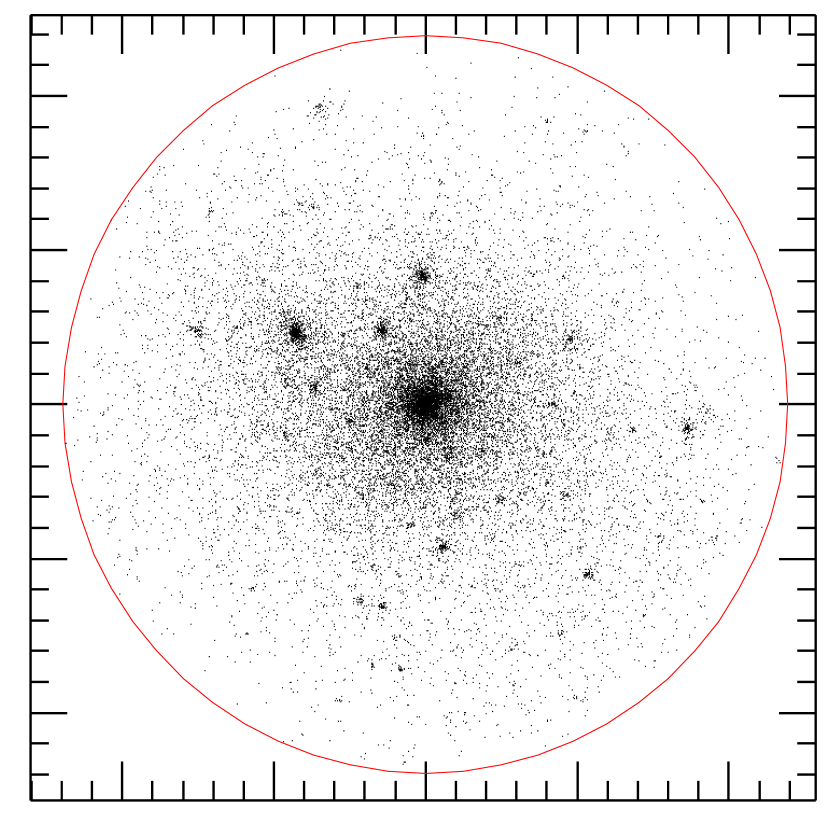
Figure 1: One of the nine clusters, at $z=0$. Only particles within the virial radius are plotted. The tick spacing is 200 kpc. Notice the amount of resolved substructure.

2.2 Identification of substructure

We identify dark matter satellites using an overdensity criterion. Each satellite groups all the particles within a sphere of mean density contrast $\rho/\rho_{b}=178$ (with $\rho_{b}$ the mean background density), centred on the local minimum of the potential energy (see Tormen 1997 for details). The corresponding radius of the satellite is its virial radius $r_{v}$.

We wish to study the fate of haloes merging with each other. To simplify this task, we focus our study on satellites accreted directly onto the main progenitor of the main halo in each simulation. The main progenitor of a halo is chosen following its merging history back in time, and selecting the main branch at each split of the merging tree (see e.g. Lacey and Cole 1993). For each simulation, this procedure provides a catalogue of satellites which will merge with the main progenitor halo at different times.

The identification time $t_{id}$ of a satellite is defined as the last time output before the satellite accretes onto the main halo progenitor. The merging time $t_{mer}$ of a satellite is the time when the satellite first crosses the virial radius of the major halo. Consecutive outputs of our simulations are separated by an interval $\Delta t\simeq 1.6$ Gyr. Therefore, the merging time for a satellite can only be bracketed between $t_{id}$ and $t_{id}+\Delta t$. We assign to each satellite a nominal merging time $t_{mer}=t_{id}+0.5\Delta t$.

After a satellite is accreted by a larger halo, its orbit and its internal structure are perturbed by the interaction with the main halo and with other substructure, and the satellite may eventually dissolve. To keep track of its motion after merging, we consider two different masses associated with the satellite: (i) the fraction of its initial mass which remains self-bound (Section 5.2), and (ii) the fraction of its initial mass within its tidal radius (Section 5.1). These definitions identify the satellite as a separate dynamical entity within the main halo.

Figure 2: Snapshots of three mergers. The circle denotes the virial radius of the parent halo. Only the particles initially within the virial radius of the satellite are plotted in each frame. To give an idea of our resolution, the satellite in the third example is formed by 68 particles, of which 51 are still self-bound in the final output.

The simulations were run for a Hubble time, i.e. $\approx 13$ Gyr for our cosmological model. Because we consider satellites which merged between $z\simeq 2.8$ and $z\simeq 0.07$, we can follow them within the cluster for up to $\sim 11$ Gyr, depending on their merging time. We limit the present analysis to satellites with $N\geq 30$ particles within $r_{v}$ at $t_{mer}$, in order to reduce the importance of numerical effects on the results. The complete set of nine simulations yields 461 satellites satisfying this constraint.

3 Tidal forces and dynamical friction

In this section we review qualitatively the physical processes dissolving the substructure.

Dynamical friction drives satellites towards energy equipartition with the smooth distribution of the cluster particles. Satellites are more massive than single particles, hence they are slowed down, their orbits shrink and become more circular as the satellites lose energy and angular momentum. Eventually the satellites are deposited in the center of the cluster potential well.

Two different types of tidal forces must be considered during the infall of satellites onto a cluster: (1) global tides caused by the interaction with the main halo, and (2) tides caused by encounters between satellites. Global tides unbind mass from the satellite in favour of the deeper potential well of the main halo. For almost circular orbits this effect is relatively mild, and only the mass in the outskirts of the halo is stripped off. Conversely, satellites on very eccentric orbits pass through the cluster core, and are completely evaporated by tidal shocks. Besides global tides, close encounters with other satellites convert orbital energy into internal energy, causing collisional stripping and eventually disruption.

Dynamical friction and tides are in action at the same time; however they have somewhat different effects on a satellite. Dynamical friction mostly influences the orbit of a satellite, by always reducing the orbital energy and angular momentum, making satellites more susceptible to global tides. Close encounters between satellites within the cluster change both the satellite orbit and its internal structure. Orbits are modified randomly, with no predictable net effect, and a satellite may either lose part of its mass or even capture mass from the perturber. Global tides mainly affect the internal structure of satellites.

Figure 2 shows three examples of mergers which roughly correspond to the extreme behaviors found in the simulations. They belong to the same simulation and correspond to three satellites which merged with the main cluster at the same redshift $z=0.9$. In the first row the satellite and the main halo have mass ratio $0.5$. For massive mergers like this one, dynamical friction is very efficient, and the satellite is driven to the center of the main halo in a very short time, almost regardless of the satellite initial orbit. The accreted satellite is also heated by the tidal shock caused by the potential of the main halo and possibly by close encounters with other satellites. However, due to its relatively large initial size, a significant part of its mass is confined within its original virial radius $r_{v}$. In the second and third row the mergers have a much smaller mass ratio, of the order of $0.01$. For this mass ratio, dynamical friction time is longer than a Hubble time, and tidal forces essentially determine the disruption or survival of a satellite. In the second example the satellite experiences a close encounter with another satellite inside the main cluster, and evaporation is immediate. In the third example, the orbit avoids both the cluster core and collisions with other satellites, allowing a much longer survival time. Therefore, the disruption or survival of a satellite depends on the balance between its initial orbit, close encounters with other haloes, and the efficiency of dynamical friction.

4 Evolution of orbits

4.1 Orbits of satellites

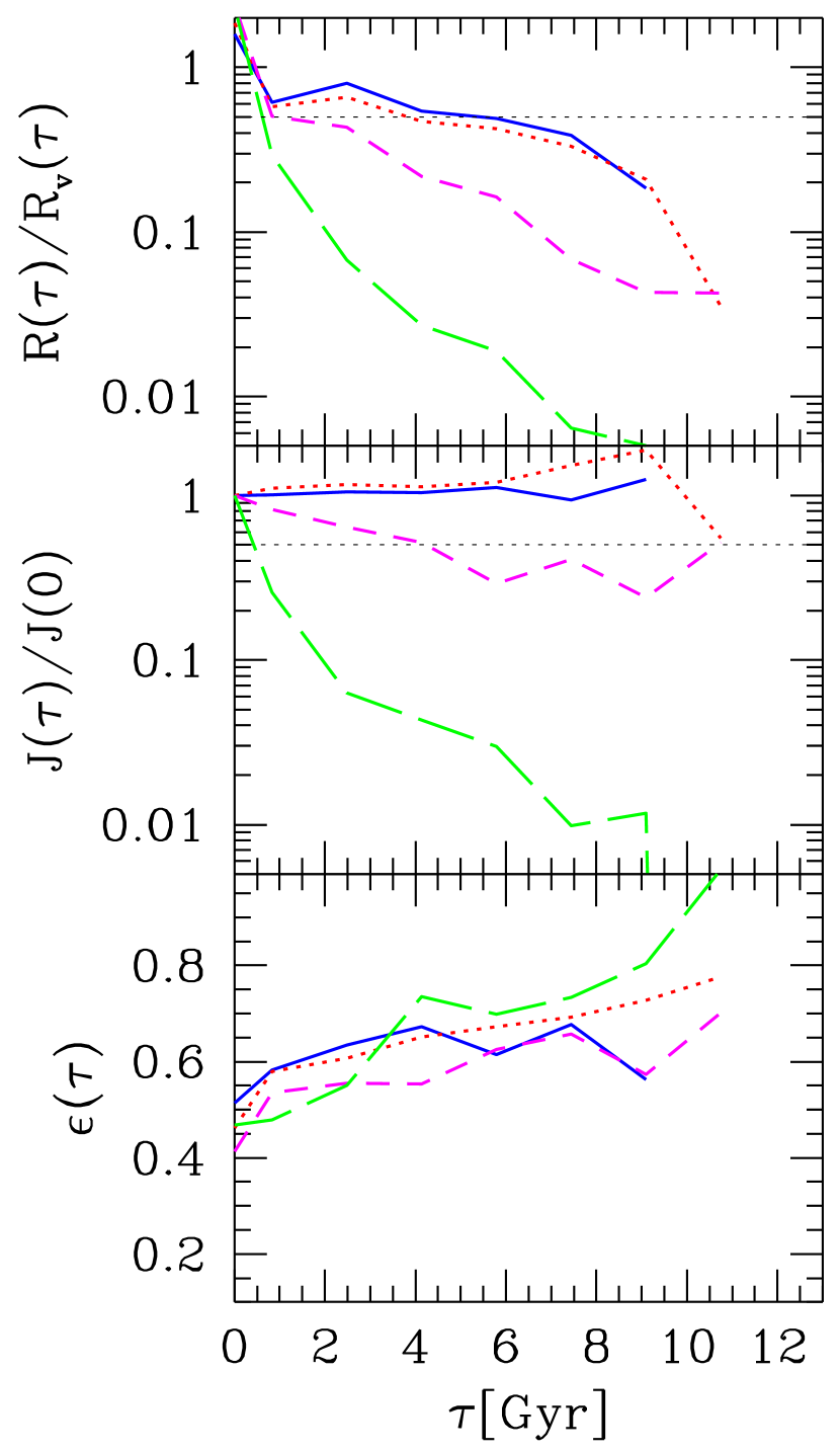
Figure 3: Evolution of orbits: distance, angular momentum, and circularity. Solid, dotted, short-dashed and long-dashed lines are for $m_{v}/M_{v}\in(0.00,0.01]$, $(0.01,0.05]$, $(0.05,0.20]$, $(0.20,1.00]$, respectively, where $m_{v}/M_{v}$ is the ratio between the satellite mass and the main halo mass at merging time. The light dotted line is at half of the initial distance and angular momentum.

In this section we study the systematic orbital decay experienced by satellites after crossing the virial radius of the main cluster. We consider all the time outputs after the merging time $t_{mer}$ and calculate the main orbital parameters for each $\tau\equiv t-t_{mer}$. Figure 3 shows the results. To show the dependence of the orbital decay on the satellite mass, we consider four subsets, according to the ratio $m_{v}(t_{mer})/M_{v}(t_{mer})$ between the satellite mass $m_{v}(t_{mer})$ and the mass $M_{v}(t_{mer})$ of the main cluster at merging time. We then calculate the median value of the parameters over the satellite distribution for each mass bin and for each $\tau$.

The top panel of Figure 3 displays the evolution of the mean distance $R(\tau)$ of a satellite from the cluster center. Note that distances at a given time are in units of the virial radius of the main halo at that time. Therefore the median distance decreases both because of dynamical friction and because of the increasing size of the main halo. Interpreting the figure with this caveat, we observe that the orbital decay is faster for more massive satellites, as expected from dynamical friction. The time required to halve the mean orbital distance is roughly 5 Gyr for satellites with $m_{v}/M_{v}\leq 0.01$, 4 Gyr for $0.01<m_{v}/M_{v}\leq 0.05$, and less than 1 Gyr for $m_{v}/M_{v}>0.05$. Due to the mass cutoff at 30 particles, no satellite was accreted 11 Gyr before the final time in the smallest mass bin. Therefore the solid curve is less extended than the others. It does not mean that the distance drops to zero at $\tau\simeq 11$ Gyr.

The second panel shows the evolution of the orbital angular momentum. This quantity is almost conserved for satellites with $m_{v}/M_{v}\leq 0.05$, while the halving time is 4 Gyr for $0.05<m_{v}/M_{v}\leq 0.20$, and less than 1 Gyr for $m_{v}/M_{v}>0.2$.

The bottom panel shows the evolution of the orbital circularity $\epsilon$, defined as the ratio between the orbital angular momentum and the angular momentum of a circular orbit with the same energy. This parameter is a measure of the orbit shape: values of $\epsilon\sim 0$ correspond to almost radial orbits, while circular orbits have $\epsilon=1$. The energy equipartition caused by dynamical friction leads to orbital circularization, as indeed observed in the figure. However, the dependence on the satellite mass is weaker for circularization than for orbital decay and angular momentum loss. Only the most massive satellites reach complete circularization in a Hubble time.

4.2 Comparison with theory

Here we compare the actual orbits of the satellites in the $N$-body simulation with a theoretical prediction based on a simple local (Chandrasekhar 1943) prescription for dynamical friction. The theoretical orbits were calculated with time-dependent satellite masses. The orbit of each satellite was integrated in the time-dependent potential of its parent cluster as measured from the simulations. For this purpose, the potential was derived from the spherically averaged mass profile and its centre of mass was fixed. For the dynamical friction we applied a frictional force

$$f_{DF}=-{\Lambda\rho(t,r)m_{sat}(t)\over s^{3}}{\bf v}_{sat}$$ (1)

where $\rho(t,r)$ is the local halo density at the position of the centre of mass of the satellite, ${\bf v}_{sat}$ is the instantaneous velocity of the satellite, and $s$ is defined by

$$s=\max[v_{sat},v_{c}],$$ (2)

where

$$v_{c}=(M(R)/R)^{1/2}$$ (3)

is the circular velocity in the halo at the satellite position. Equation (1) is a crude approximation to the usual local Chandrasekhar formula for dynamical friction in an isotropic system (e.g. Binney & Tremaine 1987). Near the centre of the parent halo $v_{c}$ is softened by replacing $R$ with $\sqrt{R^{2}+\epsilon^{2}}$, where $\epsilon\simeq 2kpc$. The Coulomb logarithm $\Lambda$ was set to a constant ($=8$). We tried two prescriptions for the satellite mass $m_{sat}$: 1) the ‘virial’ mass $m_{v}(t)$, more exactly the mass of satellite particles within the original virial radius at the identification time; and 2) the self-bound mass $m_{b}(t)$, defined in Section 5.2. The former was found to give the best results (a similar conclusion was reached by Navarro, Frenk & White 1995), and was used for the results described.

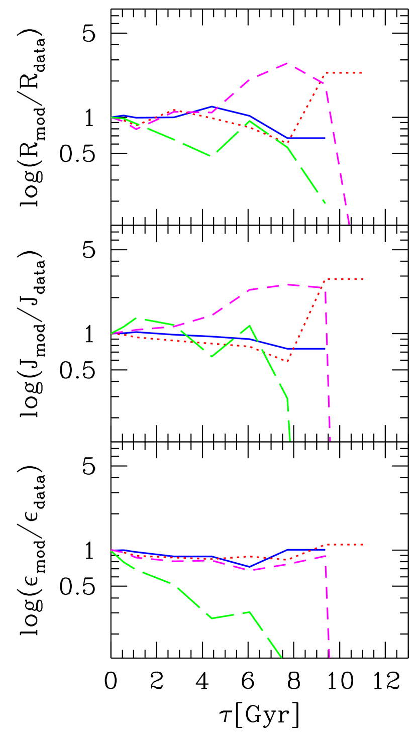
Figure 4: Evolution of orbits compared with theory assuming a simple local prescription for dynamical friction: as in Figure 3 distance, angular momentum, and circularity. Each panel shows the ratio of the theoretical prediction to the quantity measured in the simulation, in each case taking the median value over all satellites at a given time. Solid, dotted, short-dashed and long-dashed lines are for $m_{v}/M_{v}\in(0.00,0.01]$, $(0.01,0.05]$, $(0.05,0.20]$, $(0.20,1.00]$, respectively.

The results are shown in Figure 4. Here we show the ratio of the theoretically predicted to the measured quantities in terms of the median over all satellites in each mass bins (the same mass bins as defined for Figure 3). In all cases the theoretical prediction is rather good for the two smallest mass bins, and fails for the large mass satellites as they approach the centre. This is not surprising since the assumptions behind the simple orbit model break down when $M(R)$ is comparable with $m_{sat}$. The most drastic effect of the breakdown of the assumptions is the plunging of the theoretical orbits of the large satellites towards the centre of the parent cluster, with $J(\tau)$ and $\epsilon(\tau)$ tending rapidly to zero. Even for these most massive satellites, however, the evolution up to $\sim 2$ Gyr of $R(\tau)$ and (to a lesser extent) $J(\tau)$ is well enough reproduced by the theoretical calculations. Thus, the decay times can be accurately predicted.

5 Survival times

In this section we consider the global disruption of substructure. One way to define the survival time $\tau_{sur}$ of a satellite of mass $m$ is through the instantaneous mass loss:

$$\tau_{sur}=-{m(\tau)\over\dot{m}(\tau)}=-{m(\tau)\over\Delta m(\tau)}\Delta t$$ (4)

where $\Delta m(\tau)=m(\tau+\Delta t)-m(\tau)$. A satellite followed inside the cluster for $n$ time outputs will contribute $n-1$ data points to the distribution of $\tau_{sur}$. We implicitly assume that these points are statistically independent from each other. Another sensible definition of survival time $\tau_{sur}$ is simply the time taken by a satellite to completely lose its initial mass $m_{v}=m(r_{v};t_{mer})$. We will use both definitions below.

Figure 5: Left panels: evolution of tidal radii. Bold solid line is the median evolution; shaded areas include first and third quartiles. Right panels: differential (histograms) and cumulative (solid lines) distributions of the survival times defined in Equation (4) for the same mass bins of the left panels. We remind that $m_{v}$ is the virial mass of satellites at merging time $t_{mer}$, and $M_{v}$ is the virial mass of the main cluster progenitor always at $t_{mer}$.

In this section we will measure the mass of a satellite in two different ways: (1) the mass $m_{t}(\tau)=m(r_{t};\tau)$ within the satellite tidal radius $r_{t}$, (Section 5.1), and (2) the satellite self-bound mass $m_{sb}(\tau)$, (Section 5.2). Unlike $m_{t}(\tau)$, the self-bound mass $m_{sb}(\tau)$ contains information on both the positions and velocities of the particles. For both mass measures, we only consider the particles within the satellite’s virial radius $r_{v}$ at $t_{mer}$.

5.1 Tidal radius

Consider a satellite in a circular orbit at distance $R$ from the cluster center. The orbiting satellite is tidally truncated at some radius $r_{t}$, loosely speaking where the differential tidal force of the cluster is equal to the gravitational attraction of the satellite:

$$dF_{tid}(R)\equiv{\partial F\over\partial R}dR={Gm\over r_{t}^{2}}.$$ (5)

Assuming that the satellite mass $m$ and its radius $r_{t}$ are negligible compared with the cluster mass and with their relative distance $R$, i.e. $m\ll M(R)$, and $r_{t}=dR\ll R$, we readily obtain

$$r_{t}=R\left[{m\over(2-\partial\ln M/\partial\ln R)M(R)}\right]^{1/3}.$$ (6)

Therefore the tidal radius is such that the mean density of the satellite within $r_{t}$ is of the order of the mean density of the main halo within $R$. This definition captures the essence of the natural definition of $r_{t}$, defined as the distance of the center of mass of the satellite from the saddle point of the potential of the total system.

For non circular orbits, the most common situation in real life, the satellite tidal radius is rather ill-defined (e.g. King 1962; Binney and Tremaine 1987; Mamon 1987; Mamon 1993). In this case, one usually keeps Equation (6), taking for $R$ the pericentric distance of the satellite orbit. We adopt this procedure. At each time $\tau$, $r_{t}$ is the solution of the equation $\bar{\rho}_{sat}(r_{t};\tau)=\bar{\rho}_{main}(r_{p};\tau-\Delta t)$, where $\bar{\rho}_{sat}(r_{t};\tau)$ is the satellite mean density at $r_{t}$, and $\bar{\rho}_{main}(r_{p};\tau-\Delta t)$ is the mean density of the main halo at the pericenter $r_{p}$ of the orbit the satellite had at the previous time output. We compute density profiles for the satellites at each time considering only the particles within $r_{v}$ at $t_{mer}$.

We then define the survived mass of a satellite as the mass $m(r_{t};\tau)$ within its tidal radius. With this mass, Equation (4) provides our first definition of survival time $\tau_{sur}$ of a satellite. Note that the tidal radius is usually associated with the effect of global tides on a static satellite profile. We use the actual density profile of the satellite, which changes in time accordingly to all kind of interactions experienced by the satellite. Therefore, the corresponding survival times are a measure of the times taken by a satellite to be destroyed by all processes together: i.e. cluster tides, close encounters and dynamical friction.

Figure 5 shows the evolution of tidal radii $r_{t}$ and the distribution of survival times for the accreted satellites. We bin satellites into four mass bins as in Figure 3. As one could expect, tidal radii of small satellites vanish more slowly than tidal radii of massive satellites. Notice that in all mass bins $r_{t}$ drops to 30 - 50 per cent of its initial value as soon as the satellite enters the main cluster and finds itself embedded in the denser environment. Because of the sudden change in the surrounding density, particles with large kinetic energy escape the satellite. The dense core survives, and afterwards, $r_{t}$ declines to zero more gently, with an intermediate constant phase for the less massive satellites.

The corresponding survival times are displayed in the right panels. The distributions are plotted up to a Hubble time, but they have a long tail further on the right, as indicated by the cumulative distributions. Median survival times for the four mass bins are, from low to high mass, $\tau_{sur}=7$ Gyr, 5.5 Gyr, 2.4 Gyr and less than 1.5 Gyr. The fraction of survival times above 13 Gyr is 36 per cent, 30 per cent, 10 per cent and 3 per cent from low to high mass.

5.2 Self-bound mass

Another measure of the mass associated with substructure is the fraction $m_{sb}(\tau)/m_{v}(0)$ of the initial satellite mass which remains gravitationally self-bound. The self-bound mass of a satellite was defined as follows.

1. At any given time we consider only the particles which composed the satellite at its identification time.

2. We estimate the total energy of each particle summing the potential energy due to the distribution of these particles and the kinetic energy calculated in a reference frame moving with the average velocity of all particles within the original virial radius $r_{v}$ of the satellite; the reference frame is centered on the position found by the moving center technique (see Tormen et al. 1997 for details).

3. We remove all particles with positive total energy, and calculate a new center of mass and average velocity for the distribution of the remaining particles.

4. we calculate new total energies using the new set of particles and the new center of mass and velocity.

We iterate the last two steps until the number of particles with negative energy is constant. This final value gives the self-bound mass of the satellite $m_{sb}(\tau)$.

In Figure 6 we compare the evolution of the self-bound mass with the evolution of the mass within the tidal radius. Bold lines show median values, while shaded areas show the first and third quartile range of the distribution at each time $\tau$. The trend of the two estimates is similar, but the mass within $r_{t}$ is always smaller than the self-bound mass.

Figure 6: Survived mass fractions after merging. Solid and dashed lines are the median evolutions of the self-bound mass and the mass within the tidal radius, respectively. Shaded areas include first and third quartiles. Mass bins are as in Figure 5.

It is not surprising that the two definitions do not agree. In fact, they use rather different criteria to identify the satellites. The mass within the tidal radius is defined by the spatial distribution of particles alone, Eq. (6); the self-bound mass also uses information coming from the particle velocities. Because particles in the outskirt of a satellite will take roughly a free-fall time to be accelerated to the cluster velocity dispersion, they will stick to the satellite for some time after they fall outside the tidal radius, and will be counted in the self-bound mass. Thus, the estimate based on tidal radii is actually a conservatively small measure of the mass associated with the satellite.

We use the evolution of the mass within $r_{t}$ as our second estimate of survival times. Figure 6 shows that median survival times, defined by the condition: $m(r_{t};\tau_{sur})=0$, are $\tau_{sur}=7.5,$ $7.5$, $4$ and $2.5$ Gyr from small to large masses. These survival times are slightly larger than the survival times derived with Equation (4). However, they are consistent with those survival times, because both distributions have large scatter.

The longer survival time of small satellites is due to the combination of two effects: (1) smaller satellites are more compact (Tormen 1997; see also Section 7); (2) dynamical friction is less effective on smaller satellites; in fact, smaller satellites have larger distances from the cluster center (Figure 3), and suffer a weaker global tide.

These results suggest that the high force and mass resolution of our simulations overcome, at least partially, the overmerging problem which is common to dissipationless $N$-body simulations (Klypin et al. 1997). Moreover, survival of galaxy size haloes do not necessarily need dissipative simulations as usually believed (e.g. Summers et al. 1995). For example, satellites with mass ratio below $0.01$, roughly corresponding to galaxy size haloes falling into a forming cluster, have median survival time 7-$7.5$ Gyr. Thus, half of the satellites of this size, accreted by a cluster at $z\simeq 0.6-0.8$, are still “safely” orbiting within the cluster potential at $z=0$. One example is the third satellite in Figure 2. Defining survival times based on self-bound masses would result in even longer survival.

Finally, we find that survival times do not depend on the initial orbit of satellites. Radial orbits drive satellites through the cluster core where tidal forces dissolve them. However, radial orbits are rare (Tormen 1997), and our statistics is too poor to investigate this issue satisfactorily.

6 Encounters between satellites

In this section we investigate the importance of close encounters between satellites orbiting within the parent cluster. High speed close encounters have been advocated as a major mechanism for the morphological evolution of galaxies in clusters (Moore et al. 1996). The mass loss in satellite-satellite encounters depends on different parameters. Here we restrict our analysis to two quantities: the relative distance $b$ of the encounter, and the ratio $\gamma$ between the relative tangential velocity $dv_{tg}$ of the two satellites and the internal velocity dispersion $\sigma_{v}$ of the perturber. Closer (smaller $b$) and slower (smaller $\gamma$) encounters are more effective in disrupting the colliding satellites.

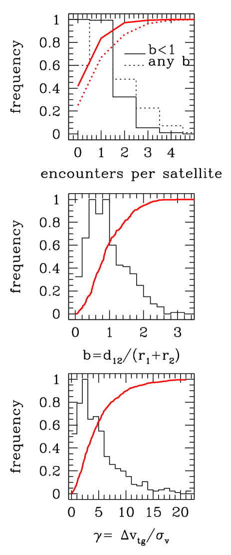
Figure 7: Parameters in satellite-satellite encounters. In each panel the thin and thick histograms indicate the differential and cumulative distribution respectively. Top panel: total number of encounters (dotted) and of penetrating encounters (solid) experienced by satellites within the main halo. Middle panel: Dimensionless relative distance of the encounter. Bottom panel: Relative tangential velocity of the encounter, in units of the internal velocity dispersion of the perturber.

Operationally, we look for encounters between satellites in the following way. Consider a satellite $i$ accreted by the main cluster at time $t_{i}$. The other satellites in the main halo are the ‘perturbers’ of satellite $i$. At each time output $t>t_{i}$, we compute the distance of satellite $i$ from all perturbers. The dimensionless relative distance between satellite $i$ and perturber $j$ at time $t$ is $b(i,j;t)=d(i,j;t)/[r(i)+r(j)]$, where $d(i,j;t)$ is the distance between the two satellites at that time, and $r(i),r(j)$ are the virial radii of the satellites at their respective merging times. The dimensionless relative velocity of the encounter $\gamma(i,j;t)=dv_{tg}(i,j;t)/\sigma_{v}(j)$ is similarly defined. The fraction of self-bound mass lost by the satellite between the time of the encounter and the next time output is

$${\Delta m(i)\over m(i)}\equiv{m_{sb}(i;t)-m_{sb}(i;t+\Delta t)\over m_{sb}(i;t)}.$$ (7)

We then consider the distribution of these quantities for all satellites, at all times $t>t_{mer}$. With the present definitions, a satellite may provide more than one data point to the distributions. We make the assumption that each satellites provides statistically independent data points in different time outputs, as was assumed in Section 5. We restrict our search to:

1. pairs of satellites retaining a non negligible fraction of their original mass at the time of the encounter: if $f_{sb}(t)=m_{sb}(t)/m_{v}(t_{mer})$ is the fraction of the initial satellite mass which remains self-bound at time $t$, we require that both $f_{sb}(i;t)$ and $f_{sb}(j;t)>0.2$.

2. satellites found within the virial radius of the main halo: $R(\tau)/R_{v}(t)<1$.

The first requirement excludes fake encounters between haloes which have already largely dissolved. The second requirement excludes time outputs when a satellites has left the main halo after a first identification. We also exclude satellites identified at the penultimate time output of the simulation, because such satellites are found within the cluster in just one output (the last one), and so we cannot calculate their mass loss.

The top panel of Figure 7 shows the differential and cumulative distributions of the number of encounters per satellite. We asked each satellite: “how many encounters did you experience which satisfy the requirements listed above?” The answer is illustrated by the dotted curves, which refer to any value of $b$. We also asked: “how many encounters with $b<1$ (referred to as penetrating encounters) did you experience which satisfy the same requirements?”. The answer is given by the solid curves. The dotted cumulative distribution shows that 25 per cent of the satellites accreted by the cluster have no encounter at all that satisfy the conditions listed above, while the remaining 75 per cent have 1 to 4 encounters. More interesting, the solid cumulative distribution shows that almost 60 per cent of all satellites have at least one penetrating encounter. We repeated the same census for satellites with $m_{v}/M_{v}<0.01$, representing galaxy-size haloes merging with a forming cluster. Almost 85 per cent of these haloes have at least one encounter, and 55 per cent have at least one encounter with $b<1$. In the other two panels we show the differential and cumulative distributions of relative distance and relative velocity for satellites having at least one encounter. The central panel illustrates that penetrating encounters are very common within the cluster: over 60 per cent of the encounters have $b<1$. The bottom panels shows that the relative velocity of the encounter is generally much larger than the internal velocity dispersion of the satellites. In fact, the satellites orbit inside the parent cluster at a speed of the order of the cluster velocity dispersion, which is much larger than the internal velocity dispersions of the satellites themselves. As a consequence, only a few per cent of the encounters have $\gamma$ of order unity. This high relative speed justifies the approximation of ignoring mass capture during the encounters, which we implicitly make when we assigning particles to a satellite.

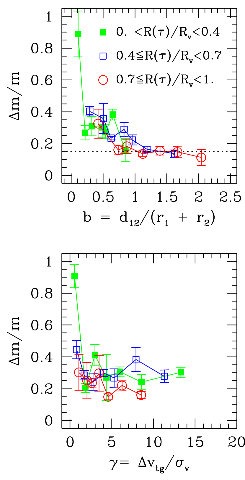
Figure 8: Top panel: median mass loss versus relative distance of the encounters $b$. Different symbols refer to encounters occurring at different distances from the center of the main halo: $0<R(\tau)/R_{v}<0.4$ (solid squares), $0.4\leq R(\tau)/R_{v}<0.7$ (open squares) and $0.7\leq R(\tau)/R_{v}<1$ (open circles). In each curve the data are binned so that each point represents the same fraction of the total encounters. Error bars are $\pm 1\sigma$ of the median. Bottom panel: median mass loss versus relative velocity of the encounter. Symbols and data binning as in the top panel.

To disentangle the mass loss due to low speed, close encounters, from the mass loss due to the tidal forces of the main halo, in Figure 8 we consider mass loss versus $b$ (top panel) and mass loss versus relative velocity (bottom panel), for encounters occurring at different distances $R(\tau)/R_{v}$ from the center of the main halo. The top panel shows that, for any fixed $b\ga 0.2$, the mass loss is roughly independent of this distance: encounters in the central region of the main halo ($0<R(\tau)/R_{v}<0.4$: solid squares) and those taking place in outer regions ($0.4\leq R(\tau)/R_{v}<0.7$: open squares, and $0.7\leq R(\tau)/R_{v}<1$: open circles) cause the same mass loss, within the statistical noise.

Notice the different range of $b$ covered by the curves: the solid symbols are concentrated at $b<1$, while encounters happening at larger distances extend further to the right. In fact, the number density of satellites grows towards the center of the main halo, increasing the chance of close encounters. The solid square at $\Delta m/m\simeq 0.9$ corresponds to head-on encounters in the inner part of the main halo, which lead to total mass disruption.

For $b\ga 1$ the curves are consistent with a roughly constant mass loss: $\Delta m/m\simeq 0.15$. If we interpret this as the average mass loss due to global tides only, then the extra mass loss is due to the encounter. The fact that mass loss increases only for penetrating encounters ($b<1$) is consistent with this explanation.

The lower panel shows that the mass loss is almost independent of the value of the relative velocity $\gamma$, and of the distance $R(\tau)/R_{v}$ from the center of the main halo. The exception is again the leftmost solid square, which corresponds to slow encounters in the core of the main halo. Encounters in the core of the main halo are both the closest and the slowest, hence the most disruptive. In fact, (1) the velocity dispersion and circular velocity of the main haloes decrease towards the center for $r/R_{v}\la 0.3$ (as shown by the radial profiles in Tormen et al. 1997), and (2) the number density of satellites increases towards the center.

On the whole, Figure 8 indicates that the mass loss during encounters between satellites depends mainly on the relative distance of the encounter, $b$, and very little on the relative velocity, because slow encounters are rare, while close encounters are frequent. Therefore, in the rest of this section we will concentrate our study on the $b$ parameter.

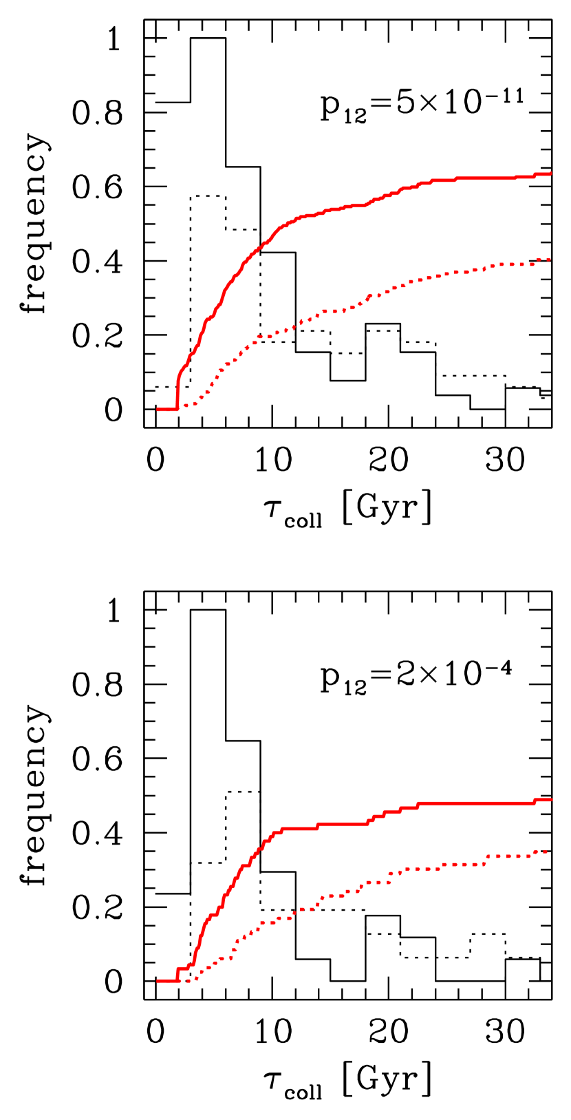
Figure 9: Differential (thin histograms) and cumulative (thick curves) distributions for the disruption time $\tau_{coll}$ from Eq. (9) due to close encounters between satellites. Top panel: Distribution for satellites of any mass. Solid and dotted lines are for $b\in[0,1)$, $[1,\infty)$ respectively. Bottom panel: Same as in top panel, for satellites in the mass range $m_{v}/M_{v}<0.01$. Values of $p_{12}$ in each panel are the Kolmogorov-Smirnov significance levels for the difference between the solid and dotted distribution.

Since we found that a constant mass loss $\Delta m/m=0.15$ is a reasonable zeroth order description of the effect of global tides, we can estimate the mass loss due only to collisions by subtracting this value from that originally measured:

$$\left({\Delta m\over m}\right)^{\prime}\equiv{\Delta m\over m}-0.15.$$ (8)

The distribution of this quantity is equivalent to the disruption time associated with the encounters:

$$\tau_{coll}=-{m(\tau)\over\dot{m}(\tau)}=-\left({m(\tau)\over\Delta m(\tau)}\right)^{\prime}\Delta t.$$ (9)

The top panel of Figure 9 shows the differential and cumulative distributions of $\tau_{coll}$ for penetrating encounters ($b<1$: solid lines) and for encounters with $b\geq 1$ (dotted lines). For this distribution we used all the data of Figure 8, excluding those contributing to the leftmost solid symbol. The median disruption time for $b<1$ is $\tau_{coll}\simeq 11$ Gyr, corresponding to a median mass loss of $(\Delta m/m)^{\prime}\simeq 0.15$. The percentage of satellites dissolved by collisions over a Hubble time is 52 per cent. On the other hand, encounters with $b\geq 1$ have negligible mass loss, and median $\tau_{coll}\gg t_{Hubble}$, a result consistent with the data shown in the top panel of Figure 8.

The bottom panel of Figure 9 shows the same statistic for satellites with $m_{v}/M_{v}<0.01$, which correspond to galaxy-size haloes falling onto a cluster. In this case mass losses due to penetrating encounters are smaller, with median value $\Delta m/m=0.05$, corresponding to a median disruption time $t\simeq 30$ Gyr, with 42 per cent of satellites being dissolved over a Hubble time.

We can use the data in the first panel of Figure 7, on the frequency of penetrating encounters in satellites, to quantify the statistical significance of encounters. Since 60 per cent of all satellites have one or more penetrating encounters, from the top panel of Figure 9 we can say that at least 30 per cent of all satellites are dissolved in 11 Gyr or less by penetrating encounters alone, and a comparable fraction is dissolved over a Hubble time. Similarly, 23 per cent of satellites with $m_{v}/M_{v}<0.01$ are dissolved by penetrating encounters in less than a Hubble time. These numbers are an estimate of mass loss and disruption time due only to penetrating encounters. Total mass losses and total survival times are those presented in Section 5.

Finally, we found that these distributions are fairly robust to variations of parameters. We obtain essentially the same results if we change the requirements on the fraction of initial satellite mass which must be self-bound at the time of the encounter, or if we only consider encounters at larger distances $R(\tau)/R_{v}$ from the center of the main halo.

7 Internal structure: mass and velocity profiles

Figure 10: Evolution of satellite mass profiles. Lines refer to different times. Time sequence is as follows: solid, dotted, short-dashed, dot-dashed, dot-dot-dot-dashed, long-dashed, bold long-dashed, solid. Note how the mass profile of the small satellites (top panels) is severely disturbed at later times (long-dashed, bold long-dashed, solid curves). Massive satellites (bottom right panel) merely expand self-similarly.

Figure 11: Same as Figure 10 for the rms velocity profiles. In the top left panel, note how particles first stream out of the satellite (dotted curve) and they increasingly thermalize with the main halo rms velocity later on (short-dashed, dot-dashed, dot-dot-dot-dashed, long-dashed, bold long-dashed curves). The rms velocity variation is abrupt, indicating that satellites are physical entities distinguishable from the main halo. The thermalization process is smoother with increasing satellite mass. The central part of the most massive satellites (bottom right panel) suffer very little cooling. Finally, note that, on average, small satellites are completely disrupted at later times (bold long-dashed, solid curves).

Here, we investigate the evolution of the internal structure of satellites. All the particles composing the satellite just before the merging time define the density and the velocity profile at each time. We can thus investigate how the internal structure of a satellite changes after the merging time, and how its mass is redistributed within the main halo.

The internal structure evolution of satellites is different for small and large mass satellites. The density of the environment surrounding a satellite suffers an abrupt change when the satellite enters the main halo. The tidal radius drastically decreases (Figure 5) and particles with enough kinetic energy escape the satellite. This process leaves low mass satellites with particles having a smaller rms velocity (Figure 11), producing an overall effect of cooling and a slight mass concentration (Figure 10). Escaped particles quickly thermalize to the main halo velocity dispersion.

From Figure 10 we see that small satellites are more concentrated than massive ones. In fact, half-mass radii for the initial profiles are at $r/r_{v}=0.2$, $0.28$, $0.35$, $0.41$ from small to large masses. For this reason, when we consider more massive satellites, the equality between the mean density of satellites and that of the main halo occurs at lower values of $r/r_{v}$. Thus, massive satellites are heated well within $r_{v}$, and the cooling effect disappears.

Moreover, the initial rms velocity of massive satellite particles is closer to the rms velocity of the main halo; thus, their kinetic energy gain is less dramatic. Mass profiles also show that the “disruption” of massive satellites is actually a mere inflating (see also Figure 2). In fact, the mass profiles are simply shifted to larger values of $r$, but their shape remains similar. On the other hand, the external shells of small satellites are violently stripped off and particles are redistributed within the main halo.

8 The fraction of halo mass in substructure

From our study it appears that only relatively small satellites can resist dynamical friction and survive in a cluster for a significant time. However, most of the mass forming a cluster comes from a few, massive objects (e.g. Tormen 1997). Therefore, it is natural to ask what is the fraction of cluster mass which, at any given time, is bound to substructure. The mass $m(r_{t};\tau)$ within the tidal radius is a measure of such fraction. By definition, the mean density within $r_{t}$ is larger than the mean density of the main cluster within the radius corresponding to the pericentre of the satellite. Therefore, the mass within the tidal radius always corresponds to an enhancement in the local mean density. We refer to this as a ‘visible’ structure. By this definition any satellite with $r_{t}>0$ is visible.

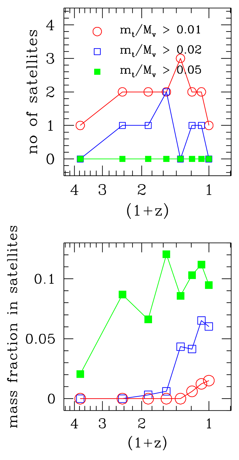
Figure 12: Fraction of cluster mass in substructure. Top panel: each curve represents the median (over the cluster sample) number of satellites found within the main halo, with mass larger than the threshold indicated in the figure, as a function of redshift. Bottom panel: Median values (over the cluster sample) of the fraction of cluster mass associated to satellites, as a function of redshift. Open circles, open squares and solid squares refer to the fraction within a sphere of radius $0.2R_{v}$, $0.5R_{v}$ and $R_{v}$ respectively. Masses are defined using tidal radii, as in Section 5.1.

The top panel of Figure 12 shows, as a function of redshift, the median number of satellites within the main halo, and with mass $m(r_{t};t)/M_{v}(t)$ above a given threshold; $M_{v}(t)$ is the virial mass of the main halo at that time. It shows that, on average, there are 2 satellites with tidally truncated mass larger than $0.01M_{v}$, one with mass larger than $0.02M_{v}$, while there is no satellite larger than $0.05M_{v}$. Note that these mass thresholds roughly correspond to satellites with radius 20, 27 and 37 per cent that of the main halo. Such objects should be fairly easily identified by e.g. weak lensing observation of the dark matter distribution in galaxy clusters (see e.g. Geiger & Schneider 1997).

The mass attached to satellites is shown in the bottom panel. The data show that, for most redshifts of interest, substructure make up on average 10 per cent of the cluster mass within $R_{v}$ (solid squares). The maximum value measured is 30 per cent. In the cluster inner regions the fraction of mass in substructure lowers dramatically (open squares and open circles refer to spheres of radius $0.5R_{v}$ and $0.2R_{v}$, respectively), due to the stronger tidal forces and to the numerical resolution. This estimate is really a lower limit, as the mass within $r_{t}$ is a conservatively low estimate of the mass of a satellite. Nevertheless most of the cluster mass is not in substructure, but is smoothly distributed inside the cluster. Therefore the issue of survival of substructure in massive haloes mainly applies to small ($m_{v}/M_{v}\la 0.05$) and compact satellites rather than to large ($m_{v}/M_{v}\ga 0.05$) ones.

9 Discussion

9.1 The extension of dark matter haloes in cluster galaxies

Studies of the kinematics of satellites of field spirals indicate that these galaxies are embedded in dark halo at least 10 times larger than the optical radius of the galaxy (Zaritsky & White 1994; Zaritsky et al. 1997). In cluster galaxies, such haloes are thought to be tidally-truncated by the cluster potential. Unfortunately, observations of this effect are very difficult. As for spiral galaxies, they are depleted of their gas by ram pressure in the intracluster medium soon after they merge, so that rotation curves cannot be measured at distances significantly larger than the optical radius (Gunn & Gott 1972, White et al. 1991). The dark haloes of ellipticals may in principle be probed by the kinematics of their globular clusters, but these objects are quite faint, so that HST observations are needed to study globulars, even in nearby cluster galaxies. If dark haloes turn out to be small enough, tidal truncation could be directly observable using weak gravitational lensing (Geiger & Schneider 1997) or observing a suitable tracer population to large radii.

Lacking observational evidence, we can at least use the results of Section 5.1 to constrain the expected radius of dark matter haloes in cluster galaxies. We can associate a galaxy radius to each dark matter satellite using the dataset of Burstein et al. (1997). These authors showed that the dynamical properties of most stellar systems, ranging from globular clusters to galaxies to galaxy groups and clusters, obey relations similar to the Fundamental Plane of ellipticals (Dressler et al. 1987; Djorgovski & Davis 1987). The ensemble of these planes, termed the cosmic metaplane, is an expression of the virial theorem, tilted by variations in mass-to-light ratio. In particular, Burstein et al. present data for $\sim 900$ elliptical and spiral galaxies, for which they derive effective radii $r_{e}$ (i.e. radii enclosing half of the total light from the galaxy) and central velocity dispersions $\sigma_{c}$.

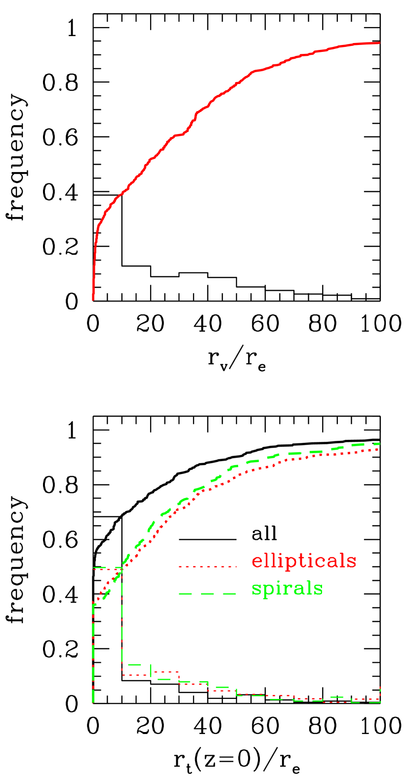
Figure 13: Radius of dark matter satellites in units of the effective radius $r_{e}$ of the host-galaxy. Top panel: virial radius, measured at merging time. Bottom panel: tidal radius, measured at the present time ($z=0$). Details about the choice of $r_{e}$ are given in the main text. Thin histograms refer to differential distributions, thick curves to cumulative distributions. Curves include all the nine cluster simulations.

Our procedure to assign $r_{e}$ to each satellite is as follows: (i) we consider all satellites infalling onto our simulated clusters, and take the one dimensional rms velocity within the virial radius, measured at merging time, as a rough estimate of $\sigma_{c}$. (ii) From the sample of Burstein et al. (1997) we select all objects having $\sigma_{c}$ within 10 per cent of the value found for the satellite. (iii) We randomly draw one of these objects and assign the corresponding value of $r_{e}$ to the satellite. This prescription can be applied also to a restricted subsample or class of observations, e.g. only the spirals or ellipticals in the Burstein et al. database. In such a case, satellites with a value of $\sigma_{c}$ not matched by any of the selected observations are excluded, leaving us with satellites in a range of $\sigma_{c}$ appropriate to the choice made.

The result of this exercise is shown in Fig 13. In the top panel we plot the differential (thin histogram) and cumulative (thick curve) distribution for the virial radius of satellites, in units of $r_{e}$, with $r_{e}$ chosen from either elliptical or spiral galaxies. This distribution gives an idea of the radius of galaxies hosted in dark matter haloes. It shows that the median virial radius for merging satellites is rhoughly 20 times larger than $r_{e}$.

In the bottom panel we plot similar distributions for the final tidal radius of satellites (i.e. measured at $z=0$). The solid distribution refers to all satellites, with $r_{e}$ chosen from galaxies, galaxy groups and galaxy clusters, in order to cover the all range of satellite masses. The dotted distribution refer to satellites associated to $r_{e}$ chosen from elliptical galaxies, while the dashed distribution has $r_{e}$ chosen from spiral galaxies. The panel shows that $\approx 35-40$ per cent of galaxy-sized dark matter satellites ever accreted by a cluster have been dissolved by the present time, i.e. they have $r_{tid}=0$ (dotted or dashed curves). The median tidal radius for galaxy-sized satellites is $r_{tid}\simeq 10r_{e}$. If we consider all satellites (i.e. also larger than galaxy-size), half of the satellites are dissolved by $z=0$ (solid curve).

Strictly speaking, these figures should be regarded as upper limits, because an increase in numerical resolution or the presence of a dense core of baryonic matter would probably facilitate the survival of satellites. The relevance of the latter effect is however not clear, as dark matter is the dominant source of gravity already at the optical radius of the galaxy (e.g. Navarro, Frenk & White 1996). Taking median values as robust estimators of the distributions, this result on the whole suggests that 50 per cent of galaxies in present-day clusters should have a dark matter halo truncated at or below $\approx 10r_{e}$, a radius close to those radii testable by e.g. high precision surface photometry. Of course, some of these galaxies will have lost a substantial part of their dark matter halo and may themselves be disrupted.

9.2 Interacting galaxies in clusters

Observations indicate that the fraction of morphologically disturbed galaxies or interacting galaxies in clusters typically increases with redshift (e.g. Lavery & Henry 1988; Oemler, Dressler & Butcher 1997). Due to the high relative speed of most encounters, illustrated in Figure 7, mergers between galaxies are expected to be rare. On the other hand, the numerical simulations of Moore et al. (1996) have shown that repeated high speed encounters between spirals, at a relative distance less than a few optical radii (e.g. $\la 50$ kpc for an $L_{*}$ galaxy) can seriously modify the galaxy morphology. This distance is also the typical separation of the interacting galaxies found by Lavery & Henry (1988).

Figure 14: Interacting satellites. The panel shows the fraction of satellites with $m_{v}/M_{v}\leq 0.01$ experiencing encounters with other satellites, as a function of redshift and binned according to the dimensionless relative distance $b$. Circles refer to encounters with $b<0.5$, open and solid squares to encounters with $b<0.2$ and $b<0.1$ respectively.

We can use the results of the analysis performed in Sections 6 and 9.1 to estimate the fraction of interacting galaxies in our simulations. Figure 14 shows the fraction of galaxy-size satellites undergoing close encounters with other satellites, as a function of redshift. We show results for dimensionless relative distances $b<0.5$, $b<0.2$ and $b<0.1$, which correspond to encounters at distances $<10r_{e}$, $<4r_{e}$ and $<2r_{e}$ if one takes the median value $r_{v}/r_{e}\simeq 20$ found in the previous section as representative. Encounters at such distances already fall in the class discussed by Moore et al. We see for example that $\approx 20$ per cent of these satellites are engaged in encounters with $b<0.5$, while $\approx 5$ per cent are having encounters with $b<0.2$, and $1-2$ per cent encounters with $b<0.1$. These figures are consistent with the $10-20$ per cent of merging and interacting galaxies observed by Oemler et al. (1997) in four clusters at $z\simeq 0.4$. The self-similarity of our simulations should ensure that such effects do not exhibit any trend with redshift, as it is indeed the case at least for $z<1$.

Our results support the claim that close encounters between galaxies in clusters are fairly frequent. The rate of encounters produced by our simulations is lower than the one invoked by Moore et al. for galaxy harrassment, as most satellites in our simulations have at most one encounters at $b<1$ (as shown in the top panel of Figure 7), and not several as required by galaxy harrassment. However, the rate we found should be considered as a lower limit, as in real clusters collisions mostly take place in the central, densest region of the cluster, where we do not have enough resolution to preserve the satellite identity. Further investigation with higher resolution simulations is required to estimate this effect.

9.3 Comparison with other work

There exist two different approaches to studying the properties of substructure within dark matter halos: (i) we can identify satellites before they merge with the main halo and keep track of their particle trajectories after merging; (ii) we can identify overdensity peaks within the main halo at each output time. The latter approach has the advantage of identifying physically motivated substructure. Moreover, this approach is equivalent to the observational procedure when it is applied to two-dimensional projections. However, this method is not straightforward if we are interested in the evolution of the substructure properties. In fact, in order to check the identity of density peaks identified at different times, we need to check whether a substantial fraction of the particles of a density peak at a later time belonged to a density peak at an earlier time (Klypin et al. 1997).

In the present work, we have eight output times for each of the nine simulations. Therefore, we use the former approach, which is more straightforward in keeping track of each satellite. The relatively large number of output times is the most important feature of our analysis. In fact, we can consistently compare the satellite orbit evolution with the dynamical friction predictions. Moreover, we can accurately estimate the evolution of the satellite internal properties as tidal effects and collisions disrupt them. This information provides a quantitative definition of the survival time.

Our analysis complements Ghigna et al. analysis. Ghigna et al. identify overdensities in a single halo simulation with higher space and force resolution than ours. Thus, they can accurately estimate the satellite density profiles, and the spatial distribution of the satellites within the main halo. On the other hand, our work has the advantage of a better statistics provided by the nine independent clusters and the use of a larger number of output times.

10 Conclusions

The results of this paper may be summarized as follows:

1. The orbital decay of haloes within galaxy clusters is consistent with the expectations of dynamical friction. Substructure are driven to the center of the main halo in less than a Hubble time if their initial mass is larger than one per cent of the mass of the main cluster.

2. Substructure retain their identity for a significant fraction of the Hubble time if their initial mass is smaller than 5 per cent of the main cluster mass. Median survival times, based on the mass within the tidal radius, are in the range [7,7.5] Gyr, [5.5,7.5] Gyr, [2.4,4] Gyr and [1,2.5] Gyr for mass ratios $m_{v}/M_{v}\in(0.00,0.01]$, $(0.01,0.05]$, $(0.05,0.20]$, $(0.20,1.00]$, respectively. However, the mass within the tidal radius is conservative, since survival times are more than 50 per cent longer when we consider the satellite self-bound mass. Smaller satellites have longer survival times for a combination of two reasons: a) they are more compact, and b) they are less influenced by dynamical friction, and avoid the cluster core.

3. Encounters between satellites within the cluster are frequent and lead to mass loss comparable to that caused by global tides. The mass loss is correlated with the relative distance and almost uncorrelated with the satellite relative velocity. In fact, slow encounters are rare, but close encounters are frequent. Almost 60 per cent of the satellites experience at least one penetrating encounter with another satellite before losing 80 per cent of their initially self-bound mass. The median mass loss per penetrating encounter is $\Delta m/m\simeq 0.15$, corresponding to a median disruption time $\tau_{coll}\simeq 11$ Gyr, due only to penetrating encounters. The same figures become $\Delta m/m\simeq 0.05$ and $\tau_{coll}\simeq 30$ Gyr for galaxy-sized satellites.

4. The evolution of the satellite internal structure depends on the satellite mass: smaller satellites easily loose their less bound particles and cool in their inner region, while larger satellites experience a global heating.

5. The fraction of cluster mass in tidally-defined substructure is 10 per cent on average within the virial radius, and lower in the inner parts. It therefore constitutes only a minor fraction of the total cluster mass.

The application of our results to galaxies in clusters requires us to specify a procedure for populating the smaller dark matter satellites with stellar material. We discuss an empirical method of assigning galaxies to haloes in Section 9. The results can be summarised as follows:

Roughly 50 per cent of galaxies in present-day clusters should have a dark matter halo truncated at or below $\approx 10r_{e}$. Some of these galaxies may themselves have been disrupted.

The fraction of satellites undergoing very close encounters, $b<0.2-0.5$, is similar to the fraction of interacting or merging galaxies in clusters at moderate redshift. Repeated close encounters, as required by galaxy harrassment, are however very rare with the present numerical resolution.

References

- [] Aguilar L.A., White S.D.M., 1985, ApJ, 295, 374
- [] Baugh C.M., Cole S., Frenk C.S., astro-ph/9703111 (submitted to ApJ)
- [Binney & Tremaine 1987] Binney J., Tremaine S., 1987, Galactic Dynamics. Princeton University Press.
- [] Burstein D., Bender R., Faber S.M., Nolthenius R., 1997, AJ, 114, 1365
- [] Chandrasekhar, S., 1943, ApJ, 97, 255
- [] Djorgovski S., Davis M., 1987, ApJ, 313, 59
- [] Dressler A., Lynden-Bell D., Burstein D., Davies R., Faber S.M., Terlevich R., Wegner G., 1987, ApJ, 313, 42
- [] Dressler A., Oemler A., Couch W.G., Smail I., Ellis R.S., Barger A., Butcher H., Poggianti B.M., Sharples R.M., 1997, ApJ, in press, astro-ph/9707232
- [geiger] Geiger, B., & Schneider, P. 1997, MNRAS, submitted
- [GMGLQS] Ghigna S., Moore B., Governato F., Lake G., Quinn T., Stadel J., in preparation
- [GG] Gunn, J.E., Gott, J.R. III, 1972, ApJ, 176, 1
- [] Lavery R.J., Henry J.P., 1988, ApJ, 330, 596
- [KWG93] Kauffmann G., White S.D.M., Guiderdoni B., 1993, MNRAS, 264, 201
- [K62] King I.R., 1962, AJ, 67, 471
- [] Klypin, A., Gottlöber, S., Kravtsov, A. V. 1997, astro-ph/9708191
- [1993] Lacey C.G., Cole S., 1993, MNRAS, 262, 627
- [Mamon87 1987] Mamon, G.A., 1987, ApJ, 321, 622
- [Mamon93 1993] Mamon, G.A., 1993, in Combes F., Athanassoula E., eds., -body Problems and Gravitational Dynamics, 188.
- [¡̧itename1996] Moore B., Katz N., Lake G., 1996, ApJ, 457, 455
- [¡̧itename1996] Moore B., Katz N., Lake G., Dressler A., Oemler A.O.Jr., 1996, Nature, 379, 613
- [¡̧itename1996] Navarro J.F., Frenk C.S., White S.D.M., 1995, MNRAS, 275, 56
- [¡̧itename1996] Navarro J.F., Frenk C.S., White S.D.M., 1996, ApJ, 462, 563
- [] Oemler A., Dressler A., Butcher H.R., 1997, ApJ, 474, 561
- [1958] Spitzer L., 1958, ApJ, 127, 17
- [] Summers F.J., Davis M., Evrard A.E., 1995, ApJ, 454, 1
- [] Tormen G., 1997, MNRAS, 290, 411
- [] Tormen G., Bouchet F.R., White S.D.M., 1997, MNRAS, 286, 865
- [Weinberg 1994] Weinberg M.D., AJ, 108, 1403
- [White 1976] White S.D.M., 1976, MNRAS, 174, 19
- [White 1976] White S.D.M., Rees M.J., 1978, MNRAS, 183, 341
- [White et al.1991] White D.A., Fabian, A.C., Forman, W., Jones, C., Stern, C., 1991, ApJ, 375, 35.
- [ 1994] Zaritsky D., White S.D.M., 1994, ApJ, 435, 599
- [ 1997] Zaritsky D, Smith R., Frenk C.S., White S.D.M., 1996, Apj submitted, astro-ph/9611207