Late Spectral Evolution of SN 1987A:
II. Line Emission
Abstract
Using the temperature and ionization calculated in our previous paper, we model the spectral evolution of SN 1987A. We find that the temperature evolution is directly reflected in the time evolution of the lines. In particular, the IR-catastrophe is seen in the metal lines as a transition from thermal to non-thermal excitation, most clearly in the [O I]6300, 6364 lines. The good agreement with observations clearly confirms the predicted optical to IR-transition. Because the line emissivity is independent of temperature in the non-thermal phase, this phase has a strong potential for estimating the total mass of the most abundant elements. The hydrogen lines arise as a result of recombinations following ionizations in the Balmer continuum during the first 500 days, and as a result of non-thermal ionizations later.
The distribution of the different zones, and therefore the gamma-ray deposition, is determined from the line profiles of the most important lines, where possible. We find that hydrogen extends into the core to . The hydrogen envelope has a density profile close to from . The total mass of hydrogen-rich gas is , of which is mixed within 2000 . The helium mass derived from the line fluxes is sensitive to assumptions about the degree of redistribution in the line. The mass of the helium dominated zone is consistent with , with a further of helium residing in the hydrogen component. Most of the oxygen-rich gas is confined to 400 – 2000 , with a total mass of . Because of uncertainties in the modeling of the non-thermal excitation of the [O I] lines, the uncertainty in the oxygen mass is considerable. In addition, masses of nitrogen, neon, magnesium, iron and nickel are estimated.
The dominant contribution to the line luminosity often originates in a different zone from where most of the newly synthesized material resides. This applies to e.g. carbon, calcium and iron. The [C I] lines, mainly arising in the helium zone, indicate a substantially lower abundance of carbon mixed with helium than stellar evolution models give, and a more extended zone with CNO processed gas is indicated. The [Fe II] lines have in most phases a strong contribution from primordial iron, and at days this component dominates the [Fe II] lines. The wings of the [Fe II] lines may therefore come from primordial iron, rather than synthesized iron mixed to high velocity. Lines from ions with low ionization potential indicate that the UV field below at least Å is severely quenched by dust absorption and resonance scattering.
1 INTRODUCTION
In Kozma & Fransson (1997; hereafter Paper I) we calculated the temperature and ionization in the ejecta of SN 1987A, which determine the line and continuum emission. Because one of the most important goals is to derive abundances and masses of the synthesized elements, these parameters are crucial for understanding the conditions in the ejecta. As will be shown in this paper, many lines have strong contributions from several abundance zones, and the emission may in fact be dominated by zones where only a small fraction of the mass of the element resides. In Paper I, it was shown that the temperature of the different abundance regions differ considerably, which puts an analysis based on a uniform temperature into question. In addition, the emission from a given zone is influenced strongly by the composition. Even a trace amount of an efficient cooler, like Ca II, can quench the emission from other lines. Finally, there is an interaction between the different abundance zones, mediated by the radiation. An obvious example is the emission from the hydrogen lines, which before 400 days is powered mainly by UV emission from the other regions absorbed by the Balmer continuum.
In spite of these complications, there has been important progress based on more limited forms of analysis. In a series of papers Li, McCray & Xu, with coworkers, (Li & McCray 1992, 1993, 1995, Li, McCray & Sunyaev 1993, Xu et al. 1992) analyze the most important emission lines from SN 1987A. Additional discussions are found in Kozma & Fransson (1992: hereafter KF92), Wang et al. 1996, and Chugai et al. (1997).
From the time evolution of the hydrogen lines Xu et al. (1992) and KF92 find that for times earlier than 400 days photoionization from the level dominates the ionization of hydrogen. In KF92 it was shown that the UV-emission from the ejecta, emitted as a result of the gamma-ray thermalization, could provide the necessary source for the Balmer continuum. Recently, Chugai et al. (1997) have modeled the time evolution of , using a time-dependent model for the hydrogen-rich gas, similar to that in this paper and in Fransson, Houck & Kozma (1996). They find that they indeed get a good fit to the observations of up to the last HST-observations at 2870 days after explosion.
An important clue to the conditions in the ejecta was obtained from an analysis of the [O I] lines, using the fact that the lines went from optically thick to thin. From this Spyromilio & Pinto (1991) and Li & McCray (1992) estimate the density of the oxygen emitting gas and the filling factor and temperature of the oxygen component. In a further paper the [Ca II] and Ca II lines are studied by Li & McCray (1993). Their main conclusion is that the calcium lines do not originate from the newly synthesized calcium, but from primordial calcium within the hydrogen-rich regions. A similar conclusion was reached by Fransson & Chevalier (1989) in the context of Type Ib supernovae.
In modeling the infrared emission lines of iron, cobalt and nickel, Li, McCray & Sunyaev (1993) conclude that the iron-rich component must have a filling factor in the core. However, they do not take the contribution of other composition regions into account. A large filling factor for the iron is also indicated from dynamical arguments (Basko 1994, Herant & Benz 1992). Finally, based on modeling of the He I m and He I m lines Li & McCray (1995) estimate the helium mass as 3 plus a similar amount mixed with hydrogen.
An interesting result by Chugai et al. (1997) is that they find that the intensity of the Fe II lines can be explained only if trapping of the positrons from 44Ti is efficient in the iron-rich parts of the ejecta. Because Coulomb scattering is not efficient enough, this puts interesting constraints on the strength of the magnetic field. At earlier epochs trapping should be more efficient.
In this paper we exploit our results in Paper I for the calculation of the line emission from SN 1987A, using a time-dependent formalism with non-thermal processes included.
Our basic model, assumptions, and physical processes included, as well as the explosion models we use, have been discussed in Paper I. A brief summary of this is given in section 2. In section 3 we discuss the calculation and importance of the line profile for constraining the density distribution, as well as the influence of dust absorption. Section 4 contains a detailed discussion of our results, while in section 5 we discuss the limitations of our modeling, and the sensitivity of our results to various assumptions and simplifications. In section 6 we discuss our results, and in section 7 we briefly summarize our main conclusions.
2 SUMMARY OF THE MODEL
Because all details of the model are given in Paper I, we only summarize the main features here. All important elements are included with the ionization stages important in this analysis. H I, He I, O I, Ca II, and Fe I-IV are treated as multilevel atoms. The equations of the ionization balance and individual level populations are solved time-dependently to include freeze-out effects. Also the energy equation is solved time-dependently, allowing for adiabatic cooling by the expansion. Radioactive decay of , and are responsible for the energy input in forms of gamma-rays and positrons. The thermalization of these is calculated by solving the Spencer-Fano equation for the abundances and electron fraction in the zone.
As input models we use the 10H model (Woosley & Weaver 1986, Woosley 1988) and the 11E1 model (Nomoto, & Hashimoto 1988, Shigeyama, Nomoto, & Hashimoto 1988, Shigeyama & Nomoto 1990, Hashimoto et al. 1989) for the abundances of the elements within the different burning zones. The ejecta is divided into a number of concentric zones of different compositions, masses and filling factors. Although simplified, this mimics the mixing of the different burning zones in the ejecta. Outside of the core we attach a hydrogen envelope with a density profile fixed to give agreement with the line profile of the line (see section 4.1.1).
3 LINE PROFILES
The best way of constraining the emissivity variation, and therefore the density distribution, comes from modeling of the line profiles of the relevant lines. For a spherically symmetric distribution, it can be shown that for an optically thin line, the emissivity, , is given by
| (1) |
(Fransson & Chevalier 1989). If is proportional to the gamma-ray deposition, and if one can consider the gamma-ray source as central this can be transformed into
| (2) |
The first of these approximations is reasonable for many lines. In particular, lines dominated by recombination, following non-thermal ionization, or lines dominated by non-thermal excitation belong to this category. Examples of the former class are the H I and He I lines, while the [O I] lines at stages later than days belong to the latter. If one line dominates the cooling of a given region this will also be a good approximation. One example of this is the [Fe II] m line from the Fe – He zone at days.
The assumption of a central gamma-ray source is doubtful at velocities outside of which there is a substantial amount of radioactive material, , in this case . A general gamma-ray deposition function, , is discussed in KF92, defined so that the mean intensity, , can be written as
| (3) |
where is the core radius. For such a general deposition function the density distribution can be obtained from
| (4) |
Approximations for are discussed in KF92 for the case of uniform distribution of the radioactive material, and outside of the core. Within the core one finds constant, and
| (5) |
At one has (as for a central source), and equation (2) is recovered. The important result is here the correspondence between the density distribution and the derivative of the line profile with respect to velocity.
Observations indicate that dust was present in the supernova ejecta at 530 days (Lucy et al. 1989, 1991). The onset of the dust formation is likely to have taken place already at days and was completed at days (Meikle et al. 1993, Whitelock et al. 1989). From the fact that the dust seemed to be opaque both in the optical and IR (Spyromilio et al. 1990, Haas et al. 1990), it has been suggested that the dust is clumpy, with very high optical depth in each clump. The latter is required to explain the presence of line asymmetries even at day 1806 (Bouchet et al. 1996). Lucy et al. (1991) estimate a covering factor of the opaque dust. A similar covering factor, , is estimated by Wooden et al. (1993) from their dust temperatures and luminosities, based on a maximum dust velocity of .
The presence of dust will decrease the escaping fluxes in lines and continua by a factor which conveniently can be parameterized by a covering factor, , applicable inside a velocity . In this paper we treat this as a pure absorption process. The thermalization of the absorbed radiation is discussed in more detail in connection with the photometry in in a subsequent paper. Here we only summarize points relevant for this paper. To model the absorption by the dust we assume a model where optically thick clumps of dust form at 350 – 600 days. In the dust formation phase it is probable that the covering factor depends on time, while later it is likely to be constant, with the optically thick dust clumps expanding with the rest of the ejecta. We therefore assume a linear increase in the covering factor from 350 to 600 days. At that time the covering factor is . Dust is likely to form only in the metal-rich parts of the ejecta (Kozasa et al. 1991). We therefore assume that only emission inside the velocity is affected by the dust absorption. Here we take , similar to the core velocity.
The dust may have important consequences for the UV intensity in the ejecta. Multiple resonance scattering increases the path length of the photons, increasing the effective probability for absorption of the UV photons by the dust in the core. This may be very efficient in decreasing the ionizing intensity in the ejecta, and introduces a major uncertainty in the calculations. The effects of a lower ionizing flux will be discussed in section 5.3. Besides absorbing the radiation the dust may also cool the gas efficiently. This was discussed in Paper I.
In our models we calculate the line profile directly from the source function, , and optical depth in the line, , as function of radius. The intensity at a given velocity is in the red wing
| (7) | |||||
where is the velocity at the maximum radius of the ejecta, , and . We have here neglected scattering of the background continuum, responsible for the P-Cygni absorption. More general cases, including this effect, are discussed in Fransson (1984). For an optically thin line without dust absorption equation (7) reduces to
| (8) |
where is the emissivity.
4 RESULTS
4.1 Line Emission
In order to compare our calculated line fluxes directly to observations we redden the calculated fluxes using =0.06 from the Galaxy and =0.10 from the LMC (Sonneborn et al. 1996). The extinction curves are taken from Savage & Mathis (1979), and Fitzpatrick (1985). In addition, as explained in section 3, the internal dust absorption in the ejecta is taken into account for the emission from the core region.
4.1.1 Hydrogen
The hydrogen lines are discussed in detail in Xu et al. (1992) and KF92, and we will therefore be fairly brief in this respect. A major issue in connection with the hydrogen emission is the density distribution in the ejecta. As we discussed in section 3, the best way of constraining this is by the line profiles. Although a complete investigation of this question is a major, separate issue, we have made some experiments with different, simplified models.
We divide the hydrogen distribution into a core contribution, most likely caused by mixing of hydrogen into the metal core, and an envelope component, which is probably relatively undisturbed by the mixing. Of these, the core component is especially uncertain. In the simulations by Fryxell, Müller, & Arnett (1991) they find a hydrogen mass of , inside of , while Herant & Benz (1992) find . Typical filling factors are %. We therefore treat the hydrogen core mass as a free parameter. For the envelope we use the density distribution of the Shigeyama & Nomoto (1990) 14E1 model, as well as our own, parameterized models.
In Figure 1 we show the observed line profile at 804 days, taken from Phillips et al. (1990), together with our models. Because only the envelope contributes at velocities greater than from the line center, we first discuss the effects of this on the line wings. The flux in the blue wing is complicated by the fact that is optically thick. Photons from the background (i.e., continuum and other weak lines) are therefore scattered by , and a P-Cygni absorption will result. Although we take optical depth effects into account for the line itself, we do not include scattering by other lines and continua. This most likely explains the asymmetry of the blue and red wings of , and for this reason we concentrate on the red wing in this discussion. Dust scattering is, however, included in the emission from the core and behind it. The bump at is caused by an unresolved [N II] line from the circumstellar ring, as can be verified from high resolution observations. A weaker bump at corresponds to the [N II] component of this doublet.
From Figure 1 it is clear that the 14E1 model gives too low a flux in the red wing. The reason is that the density profile in the envelope of this model is too steep. The 11E1 model, with a lower envelope mass, has an even steeper density gradient, and therefore does not improve the fit. For this reason we have simply parameterized the envelope distribution by , where is the density at velocity . is determined by the total mass of the hydrogen envelope in the model. The exact comparison is somewhat sensitive to the continuum level assumed. As equation (1) shows, the derivative of the line profile is, however, more relevant than the absolute level, and we find that a model, having a similar slope in the wing as the observation, is for this reason the most satisfactory model. The resulting line profile at 800 days is shown in Figure 1, and the flatter density distribution improves the fit to the red wing considerably. However, between the model has a derivative that is too steep, and the 14E1 model is closer to the observed slope. The mass within this velocity region is in the 14E1 model , while in the model the mass between is . The maximum mass in this region should therefore be close to that of the 14E1 model, and . Our favored value of the total mass outside is therefore .
Having fixed the envelope component, we now add a core contribution, which gives the additional flux needed inside . The fact that the line profile is clearly peaked () to shows that hydrogen is present at least to this velocity. We find that a fairly uniform distribution of mass in the core between gives an acceptable fit to the profile. Between we need . The mass within the core is therefore , and the total mass of hydrogen-rich gas in the ejecta . Of this is hydrogen, while most of the rest is helium.
With the hydrogen density distribution determined by the line profile, we discuss the light curves for the model with and . In Figures 2 and 3 we show the time evolution for , , , , the / ratio, the Balmer, and Paschen continua, and the H 97, and H 76 transitions. The solid line is the total calculated line flux, using a full hydrogen atom with all -states up to included (see appendix in Paper I), which should be compared to the observations. In the figures we also show the contributions from the core regions (dotted line), and the hydrogen envelope (dashed line). Of these, the contribution from the core regions dominates up to days, after which the envelope contributes most. This is a result of freeze-out, which is most pronounced, in the outer, low density, envelope regions.
In our calculations is optically thick in the core up to 1300 days. becomes optically thin in the outer parts of the envelope already at 550 days, and the entire envelope is thin at 850 days. is optically thick in the core regions up to day , while in the outer regions of the envelope becomes optically thin after 350 days. The inner envelope regions become optically thin at 700 days. The total ratio, as well as the ratios from the core and envelope regions, are shown in Figure 2. When the Balmer lines are optically thick, i.e. Case C, splits into one and one photon. As becomes thin the ratio settles at a value of 3.7 at 1200 days, slowly increasing to 4.3 at 2000 days. Taking reddening into account, the ratio should be multiplied by a factor of 1.18, resulting in an observed 4.3 at 1200 days, as seen in Figure 2.
Martin (1988) and Storey & Hummer (1995) discuss hydrogen recombination at low temperature. Martin does not take collisions into account, i.e. recombination in the low density limit. He compares calculations using an -method (the different -states are populated according to statistical weights), and an -method where he treats the -substates explicitly. In Case B he finds that at 500 K the -ratio is 2.5 and 4.2 for the and -methods respectively, showing the importance of treating the -states individually. The assumption of complete -mixing (the -method), however, becomes better for higher densities. Storey & Hummer include both individual -states, as well as collisional processes. For an electron density of cm-3, a temperature of 500 K, and Case B they find an -ratio of 3.68. The collisional processes makes the -method a better approximation and reduces the ratio. We find in our models that -mixing is accurate up to days. At later time the decreasing density causes increasing deviations from this approximation. At 1200 days this gives differences by for lines like and Pa. At the same epoch the ratio is a factor of about two higher in the model with individual -states. Therefore, at least at late time an accurate calculation requires inclusion of these effects. In our calculations at 2000 days Case B is valid, but our temperature, as well as the electron density, is lower than in the example from Storey & Hummer, resulting in our somewhat higher ratio. The effect of decreasing temperature and electron density is to increase the -ratio.
Photoionization from is never a dominant process. Instead, for days photoionization in the Balmer continuum is the most important source of ionization, as was found already in KF92 and Xu et al. (1992). Here we demonstrate this in a more realistic context, with a more self-consistent treatment of the UV-field, temperature and ionization. At days non-thermal ionization from the ground state dominates photoionization from excited levels, in agreement with KF92.
For hydrogen we include non-thermal excitations up to . For the contribution from non-thermal excitations is larger than direct recombination, except for the outermost envelope regions at later times. For and recombination dominates during most of the evolution. Later than 1000 days, however, for the two contributions are of the same order, while for the level recombinations always dominate. Within the core two-photon emission always dominates the de-population of over Ly emission. In the envelope, however, Ly emission exceeds two-photon emission.
4.1.2 Helium
The regions contributing to the He I lines (see Fig. 4) are naturally the helium, but also the iron and hydrogen regions. In our calculations we find that the fraction of the deposited non-thermal energy going into these three regions are 8%, 5%, and 60%, respectively, at around 500 days, in accordance with Table 3 in Paper I when allowance for the positron input to the Fe – He zone is made. For determination of the helium mass the distribution in velocity is extremely important, since this directly determines the gamma-ray deposition,
| (9) |
A relatively large mass, , at high velocity can therefore be difficult to detect. This is further discussed in Houck & Fransson (1996) for SN 1993J.
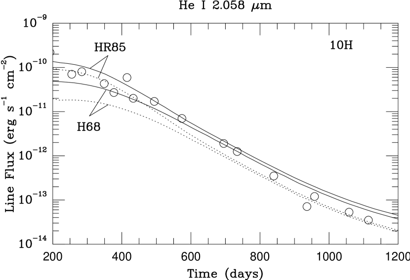
In the same way as for , we constrain the helium distribution from the line profiles. Of the He I lines the m line is best suited for this type of analysis, because of the relative absence of blending with other lines (Fig. 5). For this purpose we take the observations by Meikle et al. (1993) at 574 and 695 days, when the line is optically thin (see below). Although the line is relatively free from blends, there may still be weak lines superimposed. Also, the signal to noise is limited. The helium density distribution based on this line fit is therefore uncertain, especially for . Because of the change in flux during this time interval, we normalize the line profiles to the peak flux of the line. The total line fluxes agree well with the observations, as can be seen from Figure 4. We find that the helium density is relatively flat between , and then falling above . Therefore, most of the mass is at velocities . The continued rise of the line profile even inside of shows that there is a substantial amount of helium close to the center. The extension to is in contrast to the model by Li & McCray (1995), who use . Because most of the helium is outside of the core, only the fraction in the Fe – He zone and the helium core fraction are affected by dust absorption. In our calculations we have 0.6 of He within and 1.4 between 2000 and , i.e. a total helium zone mass of . This is the total mass in the helium zone, of which is pure helium. In addition to this, we have of helium from the hydrogen-rich regions.
Figure 4 shows the m and m light curves. The He I m line is dominated by emission from the helium regions at all times, and therefore the differences between the models are small. For the m feature, on the other hand, we find that the contribution from [S I] m is important, and actually dominates the emission for model 10H, up to 700 days. At later epochs the He I line from the helium zone dominates the light curve. Later than 1200 days the contributions from the hydrogen envelope takes over. From the hydrogen envelope, most of the emission is due to He I, but the contribution from Pa increases with time.
The flux of He I m is sensitive to the treatment of the continuum destruction probability of the line. The large abundance of carbon in the He – C zone can cause the line to be absorbed by C I. This process, and the competing processes of escape and branching to the m line, has been discussed in KF92 and by Li & McCray (1995). As was mentioned in the discussion of the continuum destruction in Paper I, we find that with the destruction probability from equation (32), in Paper I photoabsorption of the line is important only for days. The continuum destruction probability was in KF92 estimated to . The reason why continuum absorption is at all important, given the branching probability of between the m transition and the transition, is that the optical depth of the m line is high. At 300 days the optical depth is in our standard model , giving roughly equal probability of branching and absorption. After this epoch the optical depth rapidly decreases. Li & McCray (1995), on the other hand, find that up to days most photons are destroyed by this process in their He – C zone.
To study the effect of the form of the continuum destruction probability, and therefore also partial versus complete redistribution, we show in Figure 6 the light curves for both the case of continuum absorption calculated assuming only absorption within the Doppler core (eq. [32], Paper I), and for the case of absorption dominated by the damping wings of the line (eq. [33], Paper I). From this figure we see that the different assumptions give total fluxes different by a factor of at 200 days, and a factor of for the emission from the He – C zone alone. The reason for the different factors is that continuum destruction is only important in the He – C zone, and not in the hydrogen zones. The factor of can be traced directly to the continuum destruction probability. For the damping parameter of the line, , and a typical continuum to line opacity of , the Doppler case has a factor of lower destruction probability compared to the damping case. In the damping case continuum destruction is consequently important up to 500 days, in accordance with Li & McCray, although the optical depth in the m line is a factor 2 – 3 smaller. As we remarked in the discussion of the continuum destruction in Paper I, the more realistic case of partial redistribution gives a lower importance to the line wings, and a destruction probability closer to the Doppler case, and we therefore believe that this case gives the best approximation to the line flux. Chugai’s (1987) partial redistribution approximation (eq. [34], Paper I) gives for only a factor higher destruction probability than the Doppler case.
The effect of the continuum absorption can also be seen in a model, further discussed in next section, where we have replaced carbon in the helium zone by nitrogen, with an abundance of . This model has a negligible continuum destruction of the photons, and therefore higher m flux at early time. At 200 days the flux is a factor of higher than in Figure 4, decreasing to at 400 days, and at 600 days. This again confirms that mass estimates based on the m line are most reliable at days. As expected, the m line is not affected by this uncertainty. Instead, it is more sensitive to the temperature as well as the optical depth, and in addition blending with other lines.
Observations by McGregor (1988), and Meikle et al. (1993) indicate a large optical depth in the two helium lines for the first couple of years, based on the asymmetry of the line profile, or rather the blue-shifted absorption troughs. In the spectra by McGregor the m line is clearly asymmetric at 437 days, indicating an optical depth substantially larger than one. At 574 days the observation by Meikle et al. is consistent with the line being either optically thick or thin, while at 695 days the trough has clearly disappeared. In our calculations we find an optical depth larger than one in the helium zones up to 700 days. The optical depths in the hydrogen core, and envelope are somewhat smaller, and the m line becomes optically thin in these regions at 650 and 400 days respectively.
For He I m it is difficult to extract any information on the optical depth from the observations, due to the blending with other lines. In our calculations we find an optical depth greater than one in the helium region even for days. In the hydrogen regions the m line becomes optically thin at 900 days.
Li & McCray (1995) find that in order to fit the m and m emission they need of nearly pure helium and of hydrogen mixed with primordial helium. They assume a filling factor of 0.30, but point out that their calculations are not sensitive to the choice of this parameter. Our helium mass is lower than Li & McCray’s. As we have discussed above, Li & McCray have a substantially larger destruction of the photons, and therefore a lower flux in the m line than in our model. Consequently, at early time the contribution from their He – C zone is very low, and most of their flux originates at these epochs from the He – N zone. This probably explains their higher helium mass.
In most other respects, however, our calculations agree well with those of Li & McCray. In particular, we find the same distribution between the various contributions to the excitation of the and levels. Non-thermal, direct excitation and recombination, following the non-thermal ionization, give in our models roughly equal contributions to the level, each . Earlier than days thermal excitations from the gives an additional . The level has a large contribution from recombinations, before 800 days, increasing to at 1200 days. Because of the meta-stability of the level, thermal collisions contribute earlier than 800 days. At later epochs this contribution falls rapidly because of the adiabatic decrease of the temperature in the helium zone.
Li & McCray find that in the hydrogen envelope the He I state is depopulated by Penning ionizations. This is confirmed by our calculations. Photoionization from the ground state of He I is always unimportant. However, photoionization of excited levels is important for ionizing He I. Up to days the photoionization rate from excited levels in He I is somewhat higher than, or of the same order as, the non-thermal ionization rate. After 700 days the non-thermal rate slowly becomes more important. The most important photoionization source is emission from lines in the UV, and especially the He I two-photon continua.
4.1.3 Carbon and Nitrogen
Figure 7 shows the [C I] light curve. Although the shape of our light curve is in agreement with observations, the model over-produces the line by a factor of . Most of the contribution to the lines comes from the helium component, and the O – C region. The mass of the latter varies substantially between the 11E1 and 10H models, and , respectively. A possible ingredient in reducing the line strengths is the influence of CO. Liu & Dalgarno (1995) find that while only a small fraction of the carbon goes into CO, the cooling of the gas is increased by up to an order of magnitude. The temperature consequently decreases at 500 days from K without CO, to only K including CO. This can easily decrease the [C I] emission by an order of magnitude. However, although the [C I] emission from the O – C region can be killed in this way, the emission from the helium region is more difficult to quench. As Liu & Dalgarno point out, CO is efficiently destroyed by He II, and little CO is expected to form in this region. One possibility is that we have under-estimated the photoionization flux above 11.26 eV in the model, which would explain the discrepancy. Our neglect of UV scattering argues against this.
Because we have fixed the total gamma-ray deposition in the helium zone from the line profile and flux of He I m, the [C I] flux from this region should be fairly reliable. We therefore conclude that the most likely solution to the over-production of the [C I] line is that the carbon mass mixed with helium is lower than in the 11E1 and 10H models ( in the helium region in both models).
The enrichment of carbon in the helium shell occurs as a result of convection during the final helium shell burning phase (e.g., Arnett 1996). Both the time scale and the efficiency are, however, uncertain due to our limited understanding of the convection process. The amount of processed carbon mixed into the helium shell is consequently uncertain. To satisfy the observations, a decrease of the carbon mass in the helium region by a factor of 5 – 10 is required.
To check the effect of more limited mixing of carbon into the helium shell, we have replaced the He – C zone by a zone with only hydrogen burning products, as given by the He – N zone in the 10H model. The most important difference is the high abundance of nitrogen, , and low carbon and oxygen abundances, and , all by number.
This model (Fig. 8) basically extinguishes the [C I] emission from the helium zone, as expected. The total flux is now close to that observed, especially taking the likely effects of the CO-cooling in the O – C zone into account. A test of this model is to check if the emission in lines of N I and N II is now compatible with the observations. The strongest of the nitrogen lines is the [N I] multiplet. Although not discussed previously, the CTIO spectra by Phillips et al. (1990) show a clear line at this wavelength in all spectra covering this wavelength region. On day 786 the model gives a reddening adjusted flux of . Including internal dust absorption this gives a flux of . On the same day the CTIO spectrum by Phillips et al. gives a flux of for the 1.04 m line, entirely consistent within the uncertainties of the model. The model strengths of [N II] are only of the line. The blending of these with will therefore effectively hide these lines. We therefore conclude that there is evidence from the observations for a more extended He – N zone, at the expense of the He – C zone.
Phillips & Williams (1991) argue that that the [C I] ratio is on day 589. On the same day we find that this ratio in the He – C zone is , while in the O – C zone it is only . With the ’standard’ model the total ratio, which is essentially the ratio in the He – C zone, is in conflict with the observations. With the He – C zone replaced by a He – N zone, the total ratio is close to that in the O – C zone, and consistent with the observations. This provides some indirect support for our conclusions above.
4.1.4 Oxygen
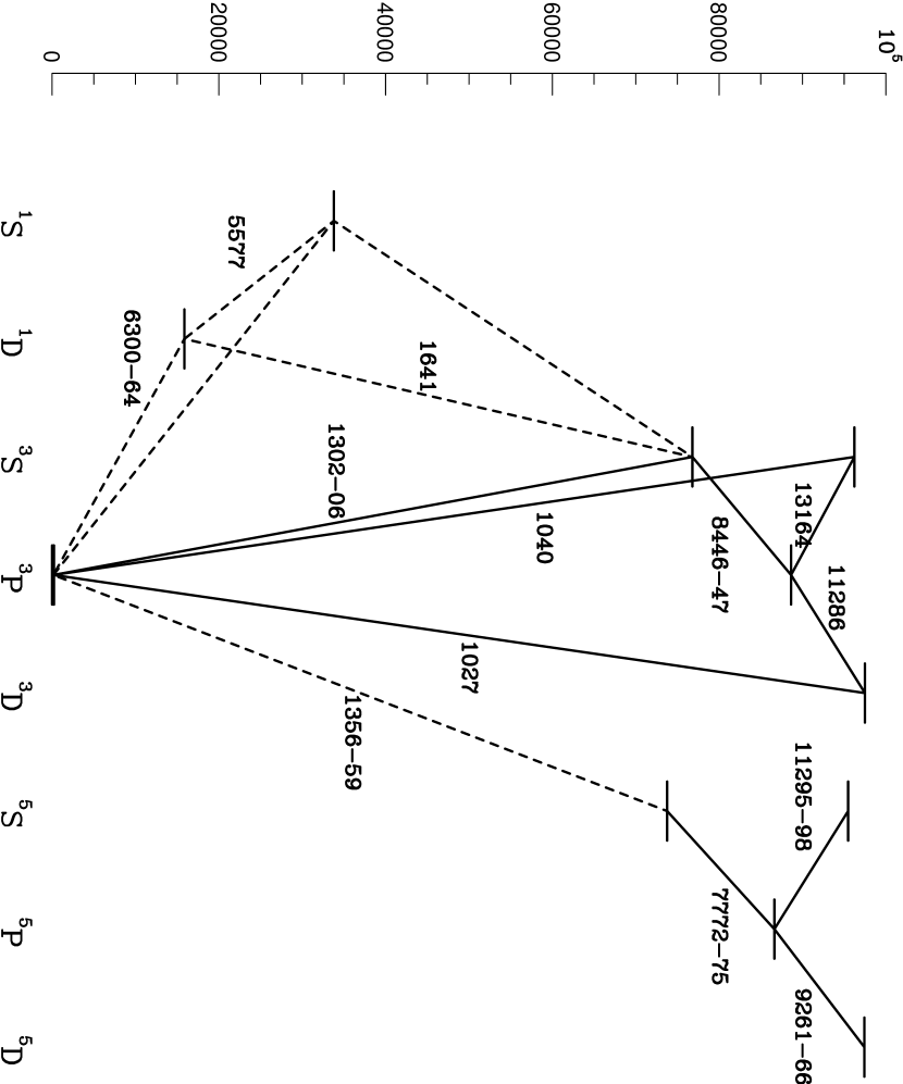
The [O I] 6300, 6364 lines are of special importance for the analysis, because they are in an easily accessible, non-blended part of the spectrum. Therefore, a complete and accurate data set exists for these lines. In addition, oxygen is the most abundant of the metals, and a good probe of the progenitor evolution and its mass (e.g., Thielemann, Nomoto, & Hashimoto 1996). For future reference we show in Figure 9 the levels and transitions included in our calculation.
Starting with the 10H model, we show in Figure 10 the light curve of [O I] 6300, 6364, together with the individual contributions from the different zones. Observations are taken from Danziger et al. (1991). The light curve can be divided into one epoch when thermal excitations of the level dominate, which lasts up to days, and one later epoch when non-thermal excitations dominate. This transition is, as explained in e.g. Fransson, Houck & Kozma (1996) and as can be seen from a comparison with Figure 2 Paper I, intimately coupled to the temperature evolution of the core. As the oxygen-rich regions undergo a thermal instability and cool to K, thermal excitation of the level effectively stops. The contributions from the hydrogen and helium-rich regions are, however, as shown in Figure 10, significant in the thermal phase. In fact, up to of the [O I] 6300, 6364 emission at 600 – 900 days comes from these components. Because of the adiabatic expansion and therefore falling temperatures of the hydrogen and helium-rich gas, the emission from both these decrease rapidly after days. This means that even if the non-thermal contribution from the core is small, it dominates after days.
In terms of the qualitative evolution we find good agreement between model calculations and observations throughout the whole period, showing without doubt that the IR-catastrophe really has taken place in the oxygen-rich gas. Quantitatively, there are, however, some disagreements. While most of the thermal phase is well reproduced, at 750 days the 10H model over-produces the [O I] luminosity by a factor of 2. The 11E1 model shows good agreement with the whole thermal part of the light curve.
The most serious flaw is in the non-thermal part. Although agreeing qualitatively with the observations, the level of the flat, non-thermal part of the curve is down by factors of 4 – 6 in the two models. As a consequence of this under-production, the transition from the thermal to the flat non-thermal light curve occurs days later than is observed. In this context we note that the observed break coincides well with the calculated transition from the O – Si – S zone, arguing for a larger contribution at late times from this.
As an illustration of the sensitivity to the assumed mass of the oxygen region, we show in Figure 11 the effect of varying the oxygen region mass by a factor of two from that of the 11E1 model, covering the range of . Other parameters of the 11E1 model are kept constant. Here we first note that the non-thermal part is under-produced even in the highest mass model, so increasing the oxygen mass does not solve that problem. The thermal part of the light curve before days is best reproduced by the standard 11E1 model, and the two other extremes probably bracket the likely range of the oxygen zone mass. Between 500 – 900 days the difference between the models is small because of the large contribution from the helium and hydrogen regions.
The total oxygen mass in the 11E1 and 10H models is roughly the same. In spite of this, the flux in the 11E1 model is only of that in the 10H model in the non-thermal part. In addition, although the mass of the O – C zone is only , compared to in the O – Si – S zone, the former contributes twice as much flux as the latter in the 10H model.
To understand this, and the general level of the light curve we have to discuss an important technical point in the excitation to the level. During the non-thermal phase, in addition to direct excitation, this level receives an important contribution from the excited level, via the line (Fig. 9). Because excitation of the level is also non-thermal, mainly by recombination following non-thermal ionizations, the basic scenario is not changed, but it can make an important quantitative difference. Normally, the de-excitation of the level is to the ground state, by the resonance multiplet, and the probability of a transition to the level in an individual transition is only . The optical depth of the resonance lines are, however, very large, increasing the effective lifetime of the level. The actual probability of a transition in the line to , compared to is
| (10) |
where the indices 1 and 2 refers to the ground state and the state, respectively. Inserting atomic parameters, and using the O I density derived by Li & McCray (1992), one finds
| (11) |
We therefore conclude that branching to dominates escape in the resonance lines up to at least days.
A further important complication is that the resonance line photons at 1302 – 1306 Å may be destroyed by photoelectric absorption by Si I, depending on the Si I abundance in the zone. If the probability of absorption dominates the branching probability, the 1302 - 1306 Å photons are destroyed, and the branching to decreases drastically. This situation is similar to that earlier discussed for helium. The probability for this to happen can be estimated from equation (32) in Paper I, as
| (12) | |||||
| (13) |
compared to the branching probability . Therefore, if , photoabsorption dominates branching to the level. The triplet contribution to the level is therefore sensitive to the chemical composition in the oxygen-rich gas. Newer models of 15 and 25 stars by Woosley & Weaver (1995) give considerably lower silicon abundances in most of the oxygen zone. Further, the estimate in equation (13) is based on continuum absorption in the Doppler profile only. As we have discussed for helium, absorption also in the damping wings can, for complete distribution, increase the destruction probability above this value. This is confirmed by the model where we used the destruction probability from equation (33) in Paper I. In this model the non-thermal level decreased to a level of of that in Figure 10. As we have already remarked, however, we believe that the Doppler case is closer to the true situation of partial redistribution.
We can now understand the origin of the somewhat paradoxical situation described above. The reason for the low contribution from the O – Si – S zone in the 10H model is the destruction of the 1302 Å photons by the abundant Si I in this zone. If it had not been for this effect the contribution from the state might have been similar in efficiency to that of the O – C zone, giving a flux proportional to the oxygen mass, and increasing the total flux by a factor . Even in the O – Ne – Mg zone in the 11E1 model, the silicon abundance is relatively high, X(Si) = , leading to the destruction of the 1302 Å photons. In spite of the larger magnesium abundance, the absorption by Si I dominates the Mg I absorption, because the photoionization cross section for Si I is almost a factor of 100 higher than for Mg I. If for some reason we have over-estimated the continuum optical depth at 1302 Å, e.g. because of too low ionization of Si I, the [O I] flux would increase. Charge transfer between O II and Si I could have this effect. In section 5.2 we discuss this quantitatively, with negative result.
To see the effect of a lower silicon abundance we show in Figure 12 the [O I] light curve for a model where we have decreased the silicon abundance in the O – Ne – Mg zone in the 11E1 model to that in the O – C region, , compared to the original . We here see that the non-thermal part indeed increases by a factor of . However, in spite of the smaller photoabsorption cross section of Mg I, in this model Mg I takes over the role of Si I, and most of the triplet contribution is also in this model quenched. An unwanted effect in this model is that there is a substantial increase in the flux between 600 – 850 days, which at this epoch destroys the agreement with the observations in the original model.
The full extent of the photoabsorption can be seen in a model, also shown in Figure 12, where we have (artificially) decreased the photoabsorption of the line to zero. Only in this model do we get a non-thermal plateau close to the observed level.
To estimate the dependence on the various parameters, and therefore more general models, it is of interest to consider a simplified model for the non-thermal [O I]6300, 6364 excitation. If we assume that the luminosity in these lines is determined only by the non-thermal excitation to the level, one can estimate the [O I]6300, 6364 luminosity by the following argument. If is the gamma-ray intensity, the absorbed energy in the oxygen component per unit volume is . Of this, a fraction will give rise to direct excitations of the level. In addition, a fraction will go into excitation of the level, via the triplet levels, as discussed above. The total energy fraction going into the level is therefore . Because collisional de-excitations at this epoch are unimportant, the total luminosity in the 6300, 6364 lines is given by
| (14) | |||||
| (15) |
where is the optical depth of the gamma-rays in the oxygen and is the total gamma-ray optical depth, both averaged over the ejecta according to the gamma-ray intensity. Both and depend on time as , and equation (15) therefore shows that, except for the dependence of on the electron fraction, a fixed fraction of the bolometric luminosity is expected in the 6300, 6364 lines, in qualitative agreement with the observations.
From our Spencer–Fano calculations for in the range . At 1000 days we find , so . Our 10H model has , so a fraction of the bolometric luminosity should come out as emission. At 1000 days (Bouchet, Danziger & Lucy 1991), and (Danziger et al. 1991), so the observed ratio is , while Menzies (1991) finds at 1000 days. This shows that unless or , direct excitation is not sufficient.
The maximum contribution from the level can be estimated by assuming that the 1302 – 1306 Å transitions have very large optical depths, and that photoabsorption is unimportant (see above). The triplet contribution to the luminosity in the 6300, 6364 lines is then
| (17) | |||||
Here, is the efficiency of ionization for O I (KF92), the effective recombination rate to the level and the total recombination rate. From calculations by Julienne, Davies, & Oran (1974) we estimate that . The factor is the fraction of the ionizations which recombine to O I. As we will see in section 5.2, can be very small if charge transfer of e.g. O II + Si I is efficient. Finally, is the fraction of the energy going into direct excitations of the triplet levels, of which most end up in the state. In KF92 the total energy into excitations in the O – Si – S zone is , of which is to the triplets, so at . The dependence on the electron fraction is roughly , for . Therefore, the maximum efficiency for excitation from the triplets is . The maximum, total efficiency is then . With and, depending on , we find , in better agreement with the observations. This argument shows that the triplet contribution is sufficient, and most likely necessary, to explain the observed non-thermal level.
The estimate above gives the luminosity for one particular hydrodynamical structure, with . To check the sensitivity of this assumption we assume that all oxygen, with a total mass , is located in a shell between velocities and . In this model , where , . With this we get
| (18) |
where is the time when the total optical depth, is unity. From light curve models Woosley, Pinto & Hartman (1989) find days. We therefore find that in the non-thermal phase
| (21) | |||||
The main parameters determining the direct excitation of the lines are therefore the oxygen mass, the velocity interval of the oxygen mass, and to a weaker degree the electron fraction in the oxygen-rich gas. Of these the oxygen distribution is probably the main uncertainty, introducing an uncertainty of up to a factor of three. Equation (21) indicates that an oxygen mass of at least is necessary to explain the observations (for ). If most of the oxygen is in a narrow velocity range, , an oxygen mass of up to may be necessary. We caution, however, that due to uncertainties in both the atomic physics and the hydrodynamics this number is not firm.
From this discussion it is obvious that there is a strong need in constraining the oxygen distribution from the observed line profile of the 6300, 6364 doublet. In Figure 13 we show the lines at 800 days for the 11E1 model (with our density distribution), including reddening and internal dust absorption. The observations are from Phillips et al. (1990). At this epoch the lines are optically thin, and the doublet components can simply be added in a ratio of 3:1. The ratio of the observed lines is considerably smaller than the expected value of 3.0 in the optically thin limit. A reason for this may be an additional contribution from the Fe I line, which in our models is of the [O I] line. The exact level of the Fe I line is uncertain because of the uncertain UV-radiation field, and it is likely that it could explain the full discrepancy.
In the velocity range there is a fairly good agreement with the observed slope of the line profile, indicating a realistic density distribution. At velocities the observations show a clear wing to , considerably stronger than in the model. There may be two reasons for this. Either the oxygen abundance in the hydrogen envelope is larger than assumed in the model, or there is mixing of a small amount of processed oxygen to these velocities. The abundances in the hydrogen envelope is set by observations of the ring of SN 1987A (Fransson et al. 1989, Sonneborn et al. 1996), and should be reliable. It would require very special conditions for the oxygen abundance in the envelope to be larger than that in the ring, which probably originates from a layer external to the envelope of the progenitor. We therefore believe that the most likely solution is the presence of some high velocity processed oxygen in the ejecta.
The observed line profile is more peaked for than the model. Our innermost oxygen zone, containing , is at , and it is clear that there is oxygen present down to at least . A better fit would be obtained if the same mass of oxygen-rich gas was mixed uniformly between . The total flux should be the same and the total mass of the oxygen zone therefore similar to that in our model, , i.e. of pure oxygen.
In the same way as for the level, one expects non-thermal excitations to the level. In this case the contribution from the triplet levels is only of that to the level. The ratio of the non-thermal excitations to the and levels is at (KF92). The ratio of the luminosity to the luminosity is therefore
| (22) |
If excitations via the level for the level are unimportant, , and the ratio of the [O I] and [O I] lines is expected to be . In the opposite case, when the triplet contribution is important, , and . The relative ratio can therefore give some information about the importance of excitation via the triplet lines of [O I] . The observed flux of the 5577 line is unfortunately uncertain because of blending with other lines. An approximate analysis of the spectrum at 804 days by Phillips et al. (1990) gives , as a strong upper limit. A more realistic limit, taking the blending by other lines (the ’continuum’) into account, reduces this upper limit by a factor of two.
The O I 7774, 8446, and 9265 lines arise as a result of recombination, and in the case of the 8446 line also by Bowen fluorescence by Ly (Oliva 1993). The flux of the 7774 line is on day 804 . This is a factor of at least four stronger than observed in the day 804 spectrum by Phillips et al. (1990). Also the 8446 line is over-produced by a similar factor. However, as suggested by Oliva, its absence can probably be explained by scattering by the Ca II IR triplet. The velocity difference to the closest component is only 1836 . The photon may therefore contribute to the excitation of the Ca II triplet. We discuss this further in section 4.1.6. The Å line could be present in the spectrum. However, the peak of the observed feature is at 9234 Å, which probably excludes it from being the O I line. The flux in this line is otherwise close to that expected for the [O I] line. The wavelength is consistent with Paschen 9 – 3 . The flux of this is, however, only expected to be of that observed. There is also an excited multiplet in S I, , coinciding with the peak of the line. This transition, which we do not include, can be expected to be strong because of recombination from the Si – S zone, and we think that this may be the most likely candidate for the line. Other strong quintet lines expected would then be the and lines. At the former wavelength there is a line with a flux of of the line, while the latter coincides with the Ca II triplet.
Therefore, all the calculated O I recombination lines seem too strong, although the line could be scattered into the Ca II triplet. The K I resonance lines at 7664.9, 7699.0 Å probably account for the P-Cygni line at Å. Its width is similar in velocity to the Na I D lines. It is, however, not likely that this doublet could scatter the line, as this would probably result in a much stronger red peak of the line than observed. Instead, its total equivalent width is close to zero, as expected if it just scatters the ’normal’ background emission. The wavelength difference is also too large. The effective recombination rates to the O I lines from Julienne, Davies, & Oran (1974) are uncertain, but not by more than a factor of two, since the total recombination rate agrees within by that found by Chung, Lin, & Lee (1991). Instead, we think that charge transfer processes, not included in our model, are responsible for the quenching of the recombination lines. This is discussed in section 5.2.
Because of the large abundance and mass of oxygen, the bound-free emission continua of O I may be observable, unless quenched by charge transfer. The strongest of these are the recombination continua to the , , and levels, with edges at 4308 Å, 8053 Å, and 8098 Å, respectively. On day 800 the temperature in the oxygen zone is K, corresponding to a width of Å at 8000 Å, and Å at 4300 Å. For the and emission we estimate a flux of , corrected for reddening and internal dust, at 8000 Å. The observed continuum level at Å is , consistent with the O I continua. Also at 4300 Å the model flux, is consistent with the observations, although blending with other lines makes it difficult to define the continuum level. Unfortunately, an unambiguous identification of these continua from the observations is difficult, although especially the continuum at 8000 Å has no other obvious candidate strong enough. An identification of this would make a direct determination of the O II fraction possible, and therefore to estimate the importance of charge transfer, as well as its temperature.
4.1.5 Neon, Magnesium, Silicon, and Sulphur
The neon abundance differs in the oxygen-rich zone by a factor of between the 10H and 11E1 models. This is a result of the different convective criteria employed in the two models. Consequently, the emission in the m [Ne II] line differs considerably between the two models (Fig. 14). While the agreement with the 10H model is satisfying up to at least days, the 11E1 model over-produces the line by a factor of at days. The last observations at days are considerably lower also in the 10H model. The uncertainty in the observation by Roche et al. (1993) at this epoch, however, is considerable.
Mg I] (Fig. 15) is completely dominated by the oxygen zone in both models. Because of the higher magnesium abundance in the 11E1 model, the flux is a factor of higher in this model compared to the 10H model. The agreement with observations is considerably better in the 10H model. The Mg I] line is interesting because it is dominated by recombination, rather than collisional excitation, as is usually the case. It is therefore not as sensitive to photoionization by the uncertain UV-field as one might think (see section 5.3). The effective recombination rate of the line is, however, uncertain (see appendix in Paper I). Recombination dominates at all epochs over both thermal and non-thermal collisional excitation.
Mg II (Fig. 16) is surprisingly weak, with a flux of of , and similar to Mg I] . Before 750 days it is excited by thermal collisions, while at late time it is dominated by non-thermal excitation. The contribution is at early time dominated by hydrogen and helium regions, while in the non-thermal phase the oxygen-rich region dominates. Because of a lower Mg II fraction at late time, the line is in this phase weaker in the 11E1 model compared to the 10H model, despite a higher magnesium abundance in the former. Unfortunately, resonance scattering by the many metal lines in the UV makes the observed luminosity at days of this line uncertain. The same is true for the Mg I resonance line. In section 6 we compare it to the HST observations at 1862 days.
The 1.64 m line is most likely a blend of the [Si I] m and [Fe II] m lines. The observed, relative contributions are, however, uncertain. The [Si I] m line should be a factor 2.84 weaker than the [Si I] m line. Also this line is blended with [Fe II] and Br 13. Figure 17 shows the calculated fluxes in the 1.64 m feature, together with the individual contributions. During most of the evolution the total flux is over-estimated by a factor 2 – 3. The reason for the early over-production may be the large contribution from the O – Si – S region, which dominates at that time. A lower abundance of silicon in this region, may bring the early part into agreement with the observations. At days the [Fe II] contribution from the hydrogen region dominates in all models. The [Si I] m line is blended with Pa, and also with the wing of the He I and [S I] lines, discussed below. Therefore we do not discuss it in any detail, and just note that the fluxes given by Meikle et al. (1993) for this line are somewhat lower than those from the 10H model. The Pa flux should be small compared to the [Si I] line (Fig. 4), but the contributions from the He I and [S I] lines large.
As we have already discussed in section 4.1.2, the strong 1.08 m feature is most likely a blend of Pa, He I m and [S I] m. At days there is too high a luminosity in this feature in the 10H model (Fig. 4). The good agreement with the He I m light curve gives us confidence that the He I m is fairly accurate. The [S I] line is therefore likely to be too strong in the 10H model. This is mainly a result of the high sulphur abundance in the O – Si – S region in the 10H model.
[S I] at 1.0820 m and [S I] at 1.1306 m originate from the same upper level. The probability for emitting a m photon is 77 %, and 23 % for a m photon. From observations by Meikle et al. (1993) we estimate the flux in the feature at 1.13 m to erg s-1 cm-2 at day 695. Another possible candidate to this feature is O I m. As was mentioned in section 4.1.4, this line may arise as a result of the O I – Ly fluorescence mechanism (Oliva 1993). We have not included this process in our calculations, and can therefore not estimate the efficiency of this mechanism. Assuming the 1.13 m feature to be due to [S I] m results in a maximum estimated flux of the [S I] m line of erg s-1 cm-2. In our calculations the flux in [S I] m is and erg s-1 cm-2 for the 10H and 11E1 models, respectively. Also from this line the 11E1 model is therefore favored by the [S I] emission. As mentioned in section 4.1.4, there may be other allowed lines from S I in the spectrum, not included in our model.
4.1.6 Calcium
The light curves of the [Ca II] 7291, 7324 lines and the IR-triplet are shown in Figures 18 and 19, together with contributions from the different components. The overall agreement of the 7291, 7324 light curve with observations is for the 10H model quite satisfying, while the lines are severely under-produced in the 11E1 model. At days there is a clear tendency to under-produce the luminosity in both models. This is still more pronounced with the triplet, but here the contributions from the [C I] and O I lines also have to be included.
An interesting point is the origin of the emission at various phases, which is sensitive to the explosion model and differs between the 10H and 11E1 models. At no epoch in either model does the Si – S component, where the explosively synthesized calcium resides, dominate. Instead, either the oxygen region or the hydrogen-rich gas contribute most of the emission in the lines.
We agree with Li & McCray (1993) that little of the Ca II emission comes from the Si – S zone, although our conclusion about the origin differs somewhat from that of Li & McCray. These authors find that the Ca II lines all originate from primordial calcium in the hydrogen and helium-rich matter, with a filling factor of . Based on the likely calcium mass, they argue that the newly synthesized calcium captures too small a fraction of the total gamma-ray flux to explain the observed line strengths. Their argument rests on the assumption that calcium is the dominant element in the newly synthesized gas. This is not the case, and nucleosynthesis models show that the calcium fraction is only , with most of the mass in silicon and sulphur. Because of the efficiency of Ca II as a coolant (e.g., Fransson & Chevalier 1989), most of the cooling of this mass may in fact be done by Ca II lines. The reason for the dominance of the other regions is therefore the low total mass of the Si – S zone, compared to the other regions. In the 10H model the mass of this region is , and a fraction of only of the gamma-rays are absorbed in this gas.
As found by Fransson & Chevalier (1989), Ca II may be a strong coolant of the oxygen-rich gas, if mixing of calcium during the hydrostatic pre-explosion burning is efficient. Crudely, the critical calcium fraction for Ca II to dominate the cooling is . The extent of this mixing is determined by the convection criterion used, as well as the extent of over-shooting. In the 10H model, where the Ledoux criterion was used and over-shooting included, this mixing is important, resulting in an abundance of in the O – Si – S zone, by number. Consequently, at days the O – Si – S region dominates the 7291, 7324 contribution, while at later time the hydrogen component within the core, with unprocessed calcium, dominates. Already at 700 days the temperature in the hydrogen-rich gas is more than a factor of two higher than in the O – Si – S region, explaining the higher contribution to the Ca II emission from the former component. The slow adiabatic decrease of the hydrogen temperature makes the decline of the Ca II lines from this component relatively slow. The temperature effect is seen even more clearly in the triplet emission, which is dominated by the hydrogen core component at all times. The 11E1 model, on the other hand, has very little calcium mixed with the oxygen.
Li & McCray find that in order for the Ca II lines to be at the observed level after days, radiative pumping of the H and K lines is necessary. As is seen in Figures 18 and 19, our light curves agree fairly well with observations up to days, if all lines coinciding with the 7300 Å lines and IR-triplet are included. The O I line has a velocity difference of 1836 from the Ca II component, and 3372 from the stronger line. These lines are optically thick in both the hydrogen and oxygen components, as well as in the Si – S – Ca region. In the H-core the component is optically thick up days, while the line is optically thick in the H-envelope at up to days. The O I photons will therefore be scattered and emerge as Ca II triplet emission up to days. This justifies the inclusion of the line in the flux from the Ca II triplet, although in section 5.2 we argue that charge transfer probably decreases the 8446 flux dramatically.
At times later than days there is a clear deficiency. This is especially clear when observations from CTIO at 953 – 1149 days are included (Suntzeff et al. 1991). The observed flux in the 7300 line on day 1046 is a factor of higher than in our models, and the 8600 complex a factor of two, including O I , which may be questionable. Our models do include radiative excitation, but only by the continuum. On day 1046 the two-photon continuum flux within the region covered by the H and K lines, Å, is only , which is much lower than the total, dereddened flux in the 7300 Å lines and IR-triplet, . If we, however, for the same day extrapolate the observed average, dereddened flux on either side of the H and K lines, , to the wavelength of these lines, we can estimate the total absorbed flux by the H and K lines to , close to the total flux in the 7300 Å lines and IR-triplet. Although the flux in the interior of the ejecta may differ from the escaping flux, this strongly suggests that radiative excitation in the H and K lines is responsible for the flux in the 7300 Å lines and IR-triplet at late epochs. The fact that the fluxes of these lines follow the bolometric flux at a level does not mean that non-thermal excitation is necessary, as for the [O I] lines. If the U-band flux follows the bolometric, as is a fair approximation to the observations after days (Suntzeff et al. 1991), radiative excitation will also result in a nearly constant . In fact, using the efficiency for non-thermal excitation in KF92, one can estimate the non-thermal contribution to of the bolometric, much less than observed.
The relative intensities of the Ca II H and K lines, the 7291, 7324 lines and the IR-triplet are discussed under various conditions by Ferland & Persson (1989), Fransson & Chevalier (1989), and Li & McCray (1993). These authors find that above the H and K, as well as the IR triplet, are in LTE, and therefore mainly depend on temperature. At temperatures below K both the H and K and the IR triplet decrease rapidly with temperature. At times when radiative excitation dominates, and if thermalization of the lines can be ignored, the ratio of the 7300 Å lines and IR-triplet is expected to be , close to the observed value of at 1046 days.
4.1.7 Iron, Cobalt, and Nickel
In our model Fe I-IV are treated as multilevel atoms with 121 levels for Fe I, 191 levels for Fe II, 110 levels for Fe III, and 43 levels for Fe IV. Fe V is included only with its ground state. The atomic data, which includes new IRON project data, are discussed in the appendix in Paper I. The total recombination coefficients (Shull & Van Steenberg, 1982), and also the fractions of the radiative recombination rates going to the ground states (Woods, Shull, & Sarazin, 1981), are probably reasonably well known. However, a major uncertainty is the individual recombination rates to the excited levels of Fe I, and Fe II, which are largely unknown. We will discuss the consequences of this later.
In Figure 20 we show the light curves of the most important Fe II lines. The observational data are taken from Erickson et al. (1988), McGregor (1988), Meikle et al. (1989), Moseley et al. (1989), Haas et al. (1990), Varani et al. (1990), Spyromilio et al. (1991), Dwek et al. (1992), Jennings et al. (1993), Colgan et al. (1994), and Bautista et al. (1995).
In general we find agreement with observations to within a factor of two, or better. It should be noted that the agreement with observations at epochs earlier than days is very good, with a possible exception of the heavily blended m line. At later epochs most of the calculated lines without correction for dust absorption are a factor stronger than observed. Including this correction with a factor , as found by Lucy et al. (1991), gives a greatly improved agreement, although they are still up to a factor of over-luminous. The importance of dust was earlier noted by Colgan et al. (1994) for the m line at 640 days.
The contributions to especially the line and the near-IR m and m lines are interesting. From being dominated by the iron core at days, the contribution from unprocessed iron in the hydrogen component becomes the most important after this epoch. The same is true for the far-IR m and m lines, although the transition for these occur later. For these lines the hydrogen component is important throughout the whole period, and later than days dominates the iron core contribution. The rapid drop in the different lines from the core can clearly be seen in Figure 6 of Paper I. The dominant hydrogen contribution to the m line at late time is in line with the KAO-observation at 1153 days by Dwek et al. (1992), who find an emitting iron mass of only , consistent with primordial.
An estimate of the luminosity of the m line coming from unprocessed gas in the hydrogen to oxygen regions is given by
| (24) | |||||
where is the total mass of hydrogen, helium or oxygen-rich gas. The optical depth of the m line in these components is
| (26) | |||||
where and are the average velocities and temperatures, respectively, of the unprocessed gas, and is the filling factor of the component. We assume that K. At 400 – 600 days the typical temperature in the hydrogen and helium-rich gas is K (Paper I). Further, our line profile fits show that most of the hydrogen and helium-rich gas have velocities within . Therefore, unless clumping is high, the m line from the unprocessed iron is likely to be optically thin, as is also argued on observational grounds by Haas et al. (1990). The total luminosity of the m line on day 407 was , decreasing to on day 640 (Haas et al. 1990, Colgan et al. 1994). With , it is clear that a large fraction of the m line may originate from unprocessed iron. As Figure 20 shows, the same applies to the other [Fe II] lines, including the m and m line.
The disappearance of the iron core contribution to the near-IR [Fe II] lines was first noted by Spyromilio & Graham (1992), who correctly attributed this to the IR-catastrophe. From their last observation on day 734 they infer an Fe II mass of , and attribute the rest to iron too cold to emit in the near-IR.
While our light curves agree well with those of Li, McCray & Sunyaev (1993) for days, a major difference between our models and those of Li et al. is in the behavior of the Fe II light curves at late time. The models by Li et al. fail to explain the emission from the Fe II, Co II, and Ni II lines for t 2 yr, with too rapid a drop of especially the optical and near-IR lines at days. As a solution they suggest that photoionization by the UV continuum, especially two-photon emission, from helium surrounding the iron may solve the problem. We do not experience this problem, because of the contribution to these lines from unprocessed iron in the helium and hydrogen region. In addition, we do include photoionization in the core, and as we discuss below, this may actually give too large an effect on the state of ionization. If photoionization really was needed, there may be a more local source of UV-photons; according to the 10H and 11E1 models there is a substantial amount of helium mixed microscopically with the iron, roughly equal abundance by number (see Tables 1 and 2 in Paper I). This could result in a substantial local UV-radiation field in the iron clumps (see below).
The light curves in Figure 21 of [Co II] m, and [Ni II] m all agree as well as can be expected, given the quality of the atomic data. Up to days the contribution from the Fe – He core dominates all lines. After this epoch the Si – S contributes most of the flux of [Ni II] m up to days. Primordial nickel dominates [Ni II] m already after days, similar to the [Fe II] lines. The [Co II] line drops rapidly after days because of the low primordial cobalt abundance.
While agreement with the Fe II, Co II, and Ni II lines is satisfying, the Fe I lines are weaker in these models by several orders of magnitude. This is seen in especially the [Fe I] m emission. The under-production of the [Fe I] m line is an ionization effect, resulting from a very low predicted Fe I abundance in all regions. The typical Fe I fraction in the iron core at 400 – 600 days is only , with most of the ionization resulting from photoionization by Fe II recombination lines and the He I two-photon continuum. A similar effect is seen in the [Ni I] m line, which is under-produced by a similar magnitude. In section 5.3 we show that changes in the UV-field can have dramatic effects on the fluxes of these lines.
5 UNCERTAINTIES IN THE CALCULATIONS
5.1 Filling Factors
The filling factors we employ for the various components are uncertain. To test the sensitivity of our results to the assumed filling factors, we have run a set of models where we have varied all filling factors by a factor of two in either direction (always assuring that the total is one). The range we have investigated is therefore , , , , , and .
With regard to the temperature evolution, we find a relatively small change up to the time of the IR-instability. The epoch when this sets in varies in the metal-rich regions by days, over the whole range of filling factors. The IR-instability occurs earlier when the filling factor increases, i.e., the density decreases. This affects the epoch of the steepest part in the light curve of the different lines. Because of the importance of adiabatic cooling, the temperature of the hydrogen and helium components in the core are hardly affected at all.
Most of the hydrogen lines are insensitive to the filling factor. An exception is , which in the period 200 – 400 days increases by a factor of when decreases from 0.3 to 0.075. The insensitivity of the hydrogen lines to the filling factor is in some disagreement with Xu et al. (1992).
The [O I] lines show little dependence on the filling factors in either the oxygen or hydrogen and helium-rich regions. The non-thermal part is also unaffected by this. The discrepancies in the light curve of this line are therefore not likely to be connected to the assumed density, but rather to the chemical composition or charge transfer effects. Also [Ca II] show weak dependence on the filling factors. The exception is the contribution from the hydrogen core, which in the period 400 – 800 days decreases by a factor of up to three between and . The lower filling factor would give a better representation of the light curve. The contribution from the O – Si – S zone, however, differs considerably less as varies. Roughly the same is true for the Ca II triplet lines.
While the optical and near-IR Fe II lines, e.g., Å, m, are insensitive to both and , the far-IR lines show a higher sensitivity. Of the individual contributions to the m and m lines the hydrogen core contribution is only weakly dependent on . The Fe – He contribution, however, decreases by a factor nearly proportional to . These conclusions agree with equation (24) and equation (43) in Paper I. Contrary to Li, McCray, & Sunyaev (1993) we find that the observations agree better with a fairly low filling factor, . The reason may be our inclusion of regions other than the iron-core, and the additional Fe II emission from these.
Summarizing this discussion, we find that plausible variations of the filling factors have rather small effects, at the factor of two level, or less. Except for perhaps the far-IR [Fe II] lines, it is likely that other uncertainties, e.g., the hydrodynamics or abundances within the different components, are at the same level or worse. We are therefore somewhat cautious of drawing any far-reaching conclusions about the filling factors from this.
5.2 Charge Transfer
Charge transfer is important for both the ionization balance and the line emission. In particular, lines and continua arising as a result of recombination can be severely affected. Earlier we noted a marked over-production of the O I recombination lines. As was shown in Paper I, the O II fraction is, however, sensitive to charge transfer with Si I, with an uncertain rate. To see the effect of this in more detail we have varied the rate of Si I + O II Si II + O I in the region cm3 s-1 in our models. We find that the O I and 9265 recombination lines, as well as the O I continua, all decrease by factors of 10 – 100, corresponding to fluxes well below the upper limits from the spectra. This is obvious from the O II curve in Figure 10 of Paper I. Charge transfer between O II and Si I would therefore solve the problem with the too large O I recombination fluxes in the previous models. At the same time the problem with the non-thermal, flat part of the [O I] light curve is exaggerated, because the contribution from the triplet levels, which to a substantial part are fed by recombination, decreases too.
Because of the small change in the Si I fraction, [Si I] m does not change appreciably. In Paper I we noted that the increase in the Si I + O II charge transfer lead to a decrease in the Mg I fraction. This does, however, not change Mg I] substantially, because of the dominance of recombination. Because of the large contribution to the 8600 Å feature from the O I line without O II + Si I charge transfer (Fig. 19), the flux of this decreases in this model substantially, later than days. Photoexcitation can probably compensate for this.
Another interesting consequence of the O II + Si I charge transfer is that the Fe I fraction in the O – Si – S zone increases by several orders of magnitude, although still too low to give Fe I lines of sufficient strength. The reason for this is that the UV flux in this zone to a large extent is determined by O I and Si I recombinations. Both decrease dramatically, while the Mg I recombination radiation is not energetic enough to ionize Fe I. In principle, other charge transfer processes in the other zones could possibly increase also the total Fe I flux.
We have also tested the influence of charge transfer from excited states of He I, discussed by Swartz (1994). However, here we find that they only contribute a few percent of the total He I ionization. Charge transfer from the ground state is also unimportant for helium.
5.3 Photoionization
Resonance scattering in the hydrogen dominated envelope has been discussed by Li & McCray (1996), using a Monte-Carlo model. Although their results are sensitive to their assumed temperature, the results may be indicative to the order of magnitude in the intensity. As input spectrum they use a pure He I two-photon continuum, but do not include other sources like the H I two-photon continuum or line emission, like , O I , and Mg II, as well as recombination emission from Si I and Mg I. Nevertheless, these calculations illustrate the importance of the UV scattering.
In Li & McCray’s model at 200 days the flux is down by a factor of , while the lower temperature and density at 800 days give a factor of suppression. The intensity inside the ejecta should be larger than the emergent intensity. On the other hand, scattering by the iron-rich material in the Fe – He bubble, not considered by Li & McCray, may further increase the scattering, and decrease the intensity. Resonance scattering will decrease with time, as is shown by the increasing UV flux in the IUE-band of SN 1987A (Pun et al. 1995), as well as the emergence of clear lines in the HST-spectra at days (Wang et al. 1996, Chugai et al. 1997).
In addition to resonance scattering, which mainly redistributes the emission in wavelength, dust absorption may have strong effects for the UV intensity. The resonance trapping in the UV increases the path length, compared to the optical range, and with a covering factor of the probability for absorption may be very large. Experiments with a simplified Monte Carlo model, similar to that in Fransson (1994), confirms this.
In KF92 the different contributions to the UV emissivity were discussed in detail, using arguments based on energy input, optical depths and atomic physics. Most of the results in KF92 are confirmed by our calculations, although quantitatively the emissivity differs from KF92. The most important reason for this is the different mass distribution in the models here, based on observed line profiles, and in KF92.
In the hydrogen zone most emission comes from H I, with and two-photon emission being most important. When the optical depth in is sufficiently large the photons scatter many times, and finally emerge in the two-photon transition from the 2 2S state to the ground state (Xu et al. 1992, KF92, Fransson 1994). In the hydrogen-rich regions in the core we find that the two-photon continuum dominates over (i.e. A2γ A) at all times between 200 – 2000 days. In the hydrogen envelope, where the density is decreasing outward, dominates in the outer zones at 500 days, and by 1200 days the emission is dominating in the entire envelope. At 500 days 45 % of the total energy absorbed by the hydrogen envelope is emitted in the H I two-photon continuum.
In KF92 it was found that of the energy absorbed by helium is re-emitted as He I two-photon emission. Of the emission coming out above 11.26 eV, most is absorbed by photoelectric absorption by the C I in the helium zone. This is caused by the large carbon abundance in this zone. A large fraction of this is in turn re-emitted as C I recombination lines in the UV. Altogether, it was estimated that of the energy was emitted in the UV between 1100 – 3646 Å. This high efficiency coupled to the large relative fraction of the energy deposited in the helium zone, means that the helium zone can be the most important source for the UV-radiation field.
In these calculations we find that compared to KF92 a considerably smaller fraction of the deposited energy goes into the helium zones, only , (compared to in KF92). This is mainly due to our redistribution of the helium to higher velocities. Of the total emission from the helium zones, is emitted in the UV Å). Of this, comes from the He I two-photon continuum after days. The 1100 - 3646 Å UV-efficiency is similar to the number above, of the absorbed energy. As in KF92, we find that the 584 Å line is mainly recycled into the 2.058 m line, plus two-photon continuum, because of the higher probability of branching into the 2.058 m line, compared to escape or continuum destruction in the 584 Å line. The He I and H I two-photon continuum photons constitute the dominant sources for the UV-field in the ejecta. Up to 600 days other strong UV-lines are Mg II 2800, C II] 2326, and C I 2966, 2968.
In the oxygen region recombination emission to the ground state of Si I ( of the absorbed energy) and Mg I () at 1521 and 1621 Å, respectively, give most of the emission. Also recombination to the excited states in Si I is important (). Because our recombination model of Si I is crude, we can not predict the detailed emissivities of these lines, although most should emerge at Å.
The UV fraction from the Fe – He region is comparatively low, . Most of this emerges as He I recombination radiation to excited states, and He I two-photon continuum emission (). Because of the large optical depths most Fe II emission is degraded into optical lines.
To investigate the uncertainty in the UV radiation field we have made one calculation where all photoionization processes from the ground states of the low ionization potential elements, Na I, Mg I, Si I, Ca I, Fe I, Ni I and Co I, are switched off.
Without photoionization we now get an Fe I fraction of at 500 days, while with photoionization the Fe I fraction is . This illustrates the sensitivity of the neutral fraction of low ionization potential elements. The Co I and Ni I fractions increase correspondingly.
Our [Fe I] and [Ni I] light curves (Fig. 22) are without photoionization only a factor of two lower than the observations, but given the quality of the atomic data and the sensitivity to both UV-field and filling factor, it is not too surprising. Because the Fe I fraction is sensitive to the assumed filling factor of iron, with for , a smaller filling factor could increase the fluxes. The [Fe II] lines decrease by , corresponding to the decrease in the Fe II fraction, improving the agreement with the observations somewhat.
The Mg I] line decreases by a factor of 2 – 3 for days, in better agreement with the observations. The reason is that radiative recombination is responsible for of the flux of this line at 800 days. Because the fraction of Mg II at 800 days has decreased from to , the Mg I] flux decreases. At days the Mg I] flux is instead higher in the model without photoionization. This is consistent with a large recombination contribution to the line, which does not vary much in the two models, because . In the non-photoionization model , while it is with photoionization. Without photoionization there is therefore a substantial collisional contribution to the line, explaining the increase.
Summarizing this, there are strong indications that the UV-field, below at least Å, in the ejecta is substantially weaker than in our standard models, because of resonance scattering, in combination with branching into the optical, or, especially efficient, dust absorption. We emphasize that this uncertainty mainly affects ions with low ionization potentials, and abundances. Dominating ions, like H I, He I, O I, Mg II, Ca II and Fe II, are only affected marginally.
6 DISCUSSION
Summarizing these calculations, we find both successes and failures. Starting with the former, we find a general good qualitative agreement with the observed evolution of most lines.
The general behavior of the hydrogen and helium lines is well reproduced, although this has already been shown by previous calculations (Xu et al. 1992, KF92). Here, we have added the time dependence, which is necessary for days. In KF92 we found a deficit in the flux at late time. This has now disappeared, partly because of the freeze-out (see also Chugai et al. 1997). In addition, we include a more realistic temperature dependence, as well as a more consistent calculation of the intensity of the radiation in the Balmer continuum, which in turn determines the Balmer line fluxes.
The effects of including the time dependence are most pronounced for lines excited by thermal collisions and recombination lines, coming from regions where adiabatic cooling and freeze-out of the ionization are important. These effects cause the electron density, as well the temperature, to be larger than in steady state (Paper I). Lines dominated by recombination are affected mainly by the higher electron density compared to steady state, increasing their luminosities. Lines formed mainly by non-thermal excitation are almost unaffected. Consequently, the time dependence is seen clearest for the [Fe II] lines at late stage, when the hydrogen and helium regions dominate. In particular, the optical and near IR-lines, e.g. Å and m, increase at 1000 days by factors 3 – 4, compared to steady state. Also the m lines increase by . The H I and He I lines, however, increase by only , at the same epoch, while [O I] is almost unaffected.
A new feature of this paper is the use of the line profiles for constraining the distribution of the various components. This was discussed already in Fransson & Chevalier (1989) and in FK92, but mainly from a qualitative point of view. Here, we have shown how both the hydrogen, helium and oxygen distributions can be determined from the observations. In particular, the penetration of a substantial hydrogen mass to has been established. This has earlier been proposed in connection to light curve calculations (e.g., Shigeyama & Nomoto 1990). Also oxygen and helium are mixed to low velocities, in the case of oxygen to . In the other direction, synthesized iron is mixed outwards to at least 2000 . Conclusions about mixing of newly synthesized iron to even higher velocities should, however, be taken with caution, because of the strong contribution of primordial iron to the lines. Because of the low resolution of the spectra used, it would be desirable to repeat this analysis with data of higher quality.
When discussing the masses of individual elements, the luminosity of the different lines are of obvious interest. However, the deposition of the gamma-rays depends on the distance from the radioactive source. While the deposition per unit mass is fairly uniform inside the radioactive source, i.e. inside , it decreases like outside. The mass outside the radioactive source is therefore not well constrained, unless the wings of the lines are well reproduced. Neglect of this leads to an under-estimate of the mass.
Of the masses determined, the hydrogen zone mass is probably the most accurate, both because of good observations, and because of well-understood physics. The total mass we find, , in the hydrogen component is probably accurate to . Of this is pure hydrogen.
The quality of the line profile of the least blended of the He I lines, m, is unfortunately not ideal. Especially the wings are not very well defined. Therefore, although the mass of the helium-rich component inside is consistent with , there could be a substantial additional mass at velocities . There is also an uncertainty in the helium mass connected to the form of the continuum destruction probability used. As illustrated in Figure 6, there may, depending on this, be a factor of up to five uncertainty in the flux at early time. At days this uncertainty is considerably smaller, and this part of the light curve is therefore better suited for helium mass determinations. We again note that of helium resides in the hydrogen-rich gas.
In both the 11E1 and 10H models most of the [C I] emission originates from regions outside of the O – C shell. Although this is not the case in the model with the He – C shell replaced by a He – N shell, the influence of CO as a coolant in the O – C shell makes mass estimates based on the [C I] lines questionable. In the model where we replaced carbon by nitrogen in the helium shell, as we argue is indicated, the [N I] 1.04 m line is dominated by the He – N region. The nitrogen mass in this model is , of which is in the He – N zone.
The strength of [Ne II] m is in the 10H model dominated by the helium zone, while in the 11E1 model the O – Ne – Mg zone takes over. The flux in the [Ne II] line was in the latter over-produced by a factor of 2 – 3 later than 500 days . Therefore, the neon mass in the 11E1 model, , is too large, and can be seen as a solid upper limit. The neon mass in the oxygen zone of the 10H model, , together with in the helium zone, gives an acceptable fit to the light curve. Allowing for a factor of two uncertainty in the model, the neon mass in either of these regions, but not both, can possibly be increased by a factor of two. A best estimate is therefore , and most likely .
Masses based on Mg I] have earlier been questioned, based on the sensitivity on the far-UV radiation (c.f., Fransson & Chevalier 1989). The fact that the line is dominated by recombinations from Mg II makes this determination considerably more reliable. The magnesium mass is likely to be similar to that in the 10H model, . The main uncertainty in this comes from the adopted effective recombination rate of the line.
As we have discussed, and agreeing with Li & McCray (1993), calcium is not well constrained, because of the dominance of the zones outside of the Si – S zone for the emission in the Ca II lines.
The iron mass should be close to the value used here, certainly within a factor of two. This mass, as well as the 56Co mass, is however, more accurately determined from the bolometric light curve. The amount of stable nickel, 58Ni and 60Ni, is in our model and given the uncertainty in the atomic data for Ni II, this is consistent with the observations.
We now turn to a number of more specific points. Of special interest is to examine the sensitivity of the line emission to the nucleosynthesis. For this purpose we have for many of the lines compared the 11E1 model by Nomoto et al. and the 10H model by Woosley. First we note that the most apparent discrepancy is in [C I] , which is similar in both models. This over-production, together with the observed presence of [N I] lines, indicates a less extensive zone of He – C, replaced by a He – N zone of CNO-burning products. This illustrates that although different models agree, there may be systematic effects due to uncertainties in the input physics in the models.
The main differences between the two models are found in the Si – S, and oxygen-rich zones. In the 11E1 model, neon and magnesium are, next to oxygen, the most abundant elements, while silicon and sulphur replaces these in the 10H model. The effects of this are most prominent in the light curves of the [O I] , [Ne II] m, Mg I] , [Si I] m, and [S I] m lines.
Starting with oxygen, the thermal part of the light curve is well reproduced in both models, although the 11E1 model gives a somewhat better fit. When it comes to the non-thermal part, both models under-produce the light curve by a large factor, although 10H somewhat less than 11E1. The problem with the [O I] line is discussed further below.
[Ne II] m clearly favors the 10H model, because of the smaller neon mass in the oxygen zone, while Mg I] agrees on the average better in the 10H model. This applies especially to the 10H model where we decreased the photoionization rate to zero (section 5.3). In the 11E1 model the light curve has the right form, but is at all epochs a factor of 2 – 3 to strong.
Because of the dominance of the zones outside of the Si – S zone for the [Ca II] emission, these lines are not as sensitive to the differences in the Si – S zone between the two models, as one could otherwise have hoped. Because of the larger Ca II contribution from the O – Si – S zone in the 10H model earlier than 400 days, this model gives a higher flux and better agreement with the observations compared to the 11E1 model.
While the contribution from the Si - S zone to the [Si I] - [Fe II] m blend varies considerably, the [Si I] emission is dominated by the oxygen zone and does not differ much. The [S I] m line is in 10H over-produced by a factor of at 200 – 300 days, and favors therefore the 11E1 model.
Summarizing this evaluation, there is no clear winner. While the [S I] lines favor 11E1, [Ne II], Mg I] and Ca II lines agree better with 10H. The early evolution of the important [O I] lines may favor the 11E1 model, but because of the serious discrepancy at late time, this is not obvious. Most discrepancies are at the factor of two level, and in view of other uncertainties it is not clear how significant the differences are. One may also take the opposite view and conclude that within this factor there is good agreement with most abundances in the models.
The low level of the non-thermal plateau of the [O I] lines poses a problem for our ’standard’ models. We have already discussed various ingredients in a solution to this problem. From our analytical discussion it is obvious that an appreciable contribution to the excitation from the triplets is needed. Although the energy to the triplets is sufficient, and branching to the singlets is probable, photoabsorption of the line by Mg I and Si I decreases this mode by a large factor. As Figure 12 shows, only a decrease in the photoabsorption to near zero has an appreciable effect on the non-thermal level. Without a strong decrease of both the magnesium and silicon abundance this is difficult to achieve, unless we have under-estimated the ionization of Mg I and Si I by a large factor. In the explosion models either magnesium or silicon, or both, tend to have a high abundance in the inner oxygen region. It is somewhat ironic that the most simplified model, with only oxygen, is the most successful model for the non-thermal phase. We have, however, also seen that the maximum triplet contribution from recombination in most cases is accompanied by too strong O I recombination lines, and we have argued that charge transfer with Si I may be a solution to this.
Another possible solution to the [O I] problem would be that the electron fraction is much lower than we have calculated, because the excitation efficiency increases with decreasing electron fraction. We have already experimented with a higher density (i.e. lower filling factor), and this did not have much effect, because . Charge transfer can probably only change by factors of a few, because the recombination rates of Mg II, Si II, and Ne II are similar to that of O II. The UV field does not influence the O I emission appreciably.
A lower abundance of silicon in the O – Si – S region would help improving both the [Si I] m line, and also increase the non-thermal plateau of the [O I] lines. In fact, a general decrease of the convective mixing of elements, like silicon in the O – Si – S region and carbon in the He – C region, in connection with the shell burning stages, would probably improve the agreement with the observations considerably. It is interesting that more recent explosion models by Woosley & Weaver (1995) give lower silicon abundances. Their 15 model has and the 25 model , both lower than in the 11E1 model. These models also show that the extent of the He – C zone can vary substantially. In the 15 model the He – C zone accounts for less than half of the helium zone, with the rest is He – N. In the 25 model nearly all of the helium zone is in the form of He – C. The neon abundance is in these models higher than even in the 11E1 model, possibly creating problems.
We also remark that the exact form of the continuum destruction probability is important, and unfortunately uncertain. This is illustrated by the difference between equations (32), (33) and (34) in Paper I, where varies by factors of ten or more, depending on the value of . A further study of this for the conditions relevant for the ejecta would be of great interest.
Because most published observations were obtained during the first four years, we have in this paper concentrated on the evolution up to days. Our models are, however, calculated up to 2000 days, and we therefore briefly compare these with the HST observations by Wang et al. (1996) at 1862 days. At this epoch blending in the UV is less severe than at earlier epochs. Meaningful estimates of the fluxes of e.g. Mg I and Mg II , as well as the Balmer continuum, can therefore be obtained. From a fit to the Balmer continuum Wang et al. find a temperature at 1862 days of K. The temperature we find in the hydrogen-rich gas decreases from K in the core to K in the inner envelope and K at the highest velocities (Figures 2 and 7 in Paper I). Given the observational uncertainties, especially in the level of the ’continuum’, we find that this is in reasonable agreement with the observations.
In Table 1 we give the observed fluxes at 1862 days from Wang et al. compared to the reddening adjusted fluxes from our 10H model at the same epoch. We find the Balmer continuum flux to be a factor of two larger than observed. The latter may, however, be a lower limit because of the high level of the background flux assumed. A factor of two higher flux could well be consistent with the observations. Our flux is very close to the observed value, implying that our electron density is close to that derived from the observations. Wang et al. estimate from an electron density of , while we find in the different regions. The [O I] flux is in the model a factor of two lower than the observed. Although the discrepancy is smaller than at earlier epochs, there is still a substantial uncertainty in the model flux because of the effects discussed earlier in this section. The Mg I and Mg II lines are not resolved in the observations. The total flux of the blend is a factor of higher than the calculated value. In the future we hope to make a more detailed comparison with these observations, as well as those even later in Chugai et al. (1997).
7 CONCLUSIONS
For convenience we here summarize our main results.
-
1.
From the evolution of especially the [O I] and [Fe II] lines there is overwhelming evidence that the IR-catastrophe has occurred in the metal-rich regions at days.
-
2.
The nearly constant ratio of the [O I] luminosity and the bolometric luminosity at days shows that non-thermal excitation dominates this part of the light curve, which implies a very low temperature. The same applies to e.g. , He I m, and Mg I] , although here recombination following non-thermal ionization dominates.
-
3.
For reliable mass estimates, constraints from the line profiles have to be taken into account. Even faint line wings at high velocity may correspond to comparatively large masses. The most reliable masses are therefore those within .
-
4.
We find that the density in the hydrogen envelope is considerably flatter than in published models, decreasing like , out to . The total hydrogen zone mass is , of which is hydrogen. The mass of the hydrogen-rich gas within 2000 is .
-
5.
The helium mass is , of which is in the helium zone and in the hydrogen zone. Although the He I m line profile is uncertain, models and observations indicate that the helium emitting mass may extend to . In the center it penetrates to . Before days the light curve, and therefore the mass estimate, is sensitive to assumptions about complete versus partial redistribution.
-
6.
Our best determinations of the other masses are (N) , (Ne) , (Mg) , (58Ni + 60Ni) . The total masses of carbon, sulphur and calcium are not well determined, because of the low contributions from zones where these elements are most abundant.
-
7.
The oxygen distribution extends to , and is consistent with of oxygen enriched gas. Because of uncertainties connected with the non-thermal part of the light curve there could be a considerable uncertainty in this number, although Figure 11 gives the likely range. The [O I] line therefore remains an unsolved problem and a better understanding of this line is clearly needed.
-
8.
The extent of convective mixing of carbon into the helium-rich region is likely to be more limited than stellar evolution calculations show. Instead, a more massive zone of CNO-burning products is indicated by the observations.
-
9.
Most lines, including the O I, Ca II, and Fe II lines, have contributions from more than one component. Even trace amounts in zones with a large gamma-ray deposition may give substantial contributions to the total line fluxes.
-
10.
The [Fe II] lines have a large contribution from primordial iron, and at late epochs this component dominates, because of the IR-catastrophe in the iron core. The extended wings of the [Fe II] lines are probably produced by primordial, rather than synthesized, iron.
-
11.
Both charge transfer and photoionization effects are important for the strengths of lines from trace ions. The observations indicate strong suppression of the UV flux by dust absorption and resonance scattering.
Finally, after this paper was submitted we received a preprint by de Kool, Li, & McCray (1997) where a similar analysis and calculation is performed. In spite of detailed differences, it is comforting that the results of these two independent calculations with regard to both the physical conditions and the observed emission are very similar.
ACKNOWLEDGMENTS
We are grateful to many people for discussions at various phases of this project. In particular, John Houck and Peter Lundqvist have provided much advice on atomic data, as well as discussions. Dima Verner has provided recombination coefficients to excited levels in He I, Peter Meikle and Mark Phillips have made observational data available in readable format. We have also had many helpful discussions and comments on these papers by Eddie Baron, Roger Chevalier, Robert Cumming, Leon Lucy, Ken Nomoto, Takashi Kozasa, Jesper Sollerman, and Jason Spyromilio, and especially by Dick McCray and Hongwei Li. This research was supported by the Swedish Natural Sciences Research Council and the Göran Gustafsson Foundation for Research in Natural Sciences and Medicine.
| Line | ModelaaObserved fluxes are from Wang et al. (1996), while the modeled are from the 10H model, adjusted for reddening. All fluxes are in units of . | ObservationaaObserved fluxes are from Wang et al. (1996), while the modeled are from the 10H model, adjusted for reddening. All fluxes are in units of . |
|---|---|---|
| 18.8 | 16.6 | |
| Balmer cont. | 7.2 | 3.1 |
| [O I] 6300, 6364 | 1.2 | 2.9 |
| Mg I] 4571 | 4.6 | 2.2 |
| Mg I 2852 | 0.58 | 1.7bbTotal flux for Mg I and Mg II . |
| Mg II 2796, 2803 | 0.07 | |
References
- (1) Aitken, D. K., Smith, C. H., James, S. D., Roche, P. F., Hyland, A. R., & McGregor, P. J. 1988, MNRAS, 235, 19p
- (2) Arnett, W. D. 1996, Supernovae and Nucleosynthesis, Princeton University Press, Princeton
- (3) Basko, M. 1994, ApJ, 425, 264
- (4) Bautista, M. A., DePoy, D. L., Pradhan, A. K., Elias, J. H., Gregory, B., Phillips, M. M., & Suntzeff, N. B. 1995, AJ, 109, 729
- (5) Bouchet, P., & Danziger, I. J. 1993, A&A, 273, 451
- (6) Bouchet, P., Danziger, I. J & Lucy, L. B. 1991, AJ, 102, 1135
- (7) Bouchet, P., Danziger, I. J., Gouiffes, C., Della Valle, M., & Moneti, A. 1996, in IAU. Coll. No. 145, Supernovae and Supernova Remnants, eds. R. McCray & Z. Wang, Cambridge University Press, 201
- (8) Chugai, N. N. 1987, Astrophysics, 26, 53
- (9) Chugai, N. N., Chevalier, R. A., Kirshner, R. P., & Challis, P. M. 1997, ApJ, 483, 925
- (10) Chung S., Lin, C. C., & Lee, E. T. P. 1991, Phys. Rev. A, 43, 3433
- (11) Colgan, S. W. J., Haas, M. R., Erickson, E. F., Lord, S. D., & Hollenbach, D. J. 1994, ApJ, 427, 874
- (12) Danziger, I. J., Bouchet, P., Gouiffes, C., & Lucy, L. B. 1991, in Proc. ESO/EIPC Supernova Workshop, SN 1987A and other Supernovae, eds. I.J. Danziger & K. Kjär, (Garching: ESO), 217
- (13) Dwek, E., Moseley, S.H., Glaccum, W., Graham, J.R., Loewenstein, R.F., Silverberg, R.F., & Smith, R. K. 1992, ApJ, 389, L21
- (14) Erickson, E. F., Haas, M. R., Colgan, S. W. J., Lord, S. D., Burton, M. G., Wolf, J., Hollenbach, D. J., & Werner, M. 1988, ApJ, 330, L39
- (15) Ferland, G. J. & Persson, S. E. 1989, ApJ, 347, 656
- (16) Fitzpatrick, E. L. 1985, ApJ, 299, 219
- (17) Fransson, C., 1984, A&A, 132, 115
- (18) Fransson, C., 1994, in Supernovae (Les Houches, Session LIV 1990), eds. J. Audouze, S. Bludman, R. Mochkovitch, & J. Zinn-Justin (New York: Elsevier), 677
- (19) Fransson, C., & Chevalier, R. A. 1989, ApJ, 343, 323
- (20) Fransson, C., Houck, J. & Kozma, C. 1996, in IAU. Coll. No. 145, Supernovae and Supernova Remnants, eds. R. McCray & Z. Wang, Cambridge University Press, 211
- (21) Fransson, C., Cassatella, A., Gilmozzi, R., Kirshner, R. P., Panagia, N., Sonneborn, G., & Wamsteker, W. 1989, ApJ, 336, 429
- (22) Fryxell, B., Müller, E., & Arnett, D. 1991, ApJ, 367, 619
- (23) Haas, M. R., Colgan, S. W. J., Erickson, E. F., Lord, S. D., Burton, M. G., & Hollenbach, D. J. 1990, ApJ, 360, 257
- (24) Hashimoto, M., Nomoto, K., & Shigeyama, T. 1989, A&A, 210, L5
- (25) Herant, M., & Benz, W. 1992, ApJ, 387, 294
- (26) Houck, J. C., & Fransson, C., 1996, ApJ, 456, 811
- (27) Hummer, D. G. 1968, MNRAS, 138, 73
- (28) Hummer, D. G., & Rybicki, G. B. 1985, ApJ, 293, 258
- (29) Jennings, D. E., Boyle, R. J., Weidemann, G. R., & Moseley, S. H. 1993, ApJ, 408, 277
- (30) Julienne, P.S., Davies, J. & Oran, E. 1974, J. Geophys. Res. 79, 2540
- (31) Kozasa, T., Hasegawa, H., & Nomoto, K. 1991, A&A, 249, 474
- (32) Kozma, C., & Fransson, C. 1992, ApJ, 390, 602 (KF92)
- (33) Kozma, C., & Fransson, C. 1997, ApJ, previous paper (Paper I)
- (34) Li, H., & McCray, R. 1992, ApJ, 387, 309
- (35) Li, H., & McCray, R. 1993, ApJ, 405, 730
- (36) Li, H., & McCray, R. 1995, ApJ, 441, 821
- (37) Li, H., & McCray, R. 1996, ApJ, 456, 370
- (38) Li, H., McCray, R., & Sunyaev, R. A. 1993, ApJ, 419, 824
- (39) Liu, W. & Dalgarno, A. 1995, ApJ, 454, 472
- (40) Lucy, L. B., Danziger, I. J., Gouiffes, C., & Bouchet, P. 1989, in IAU Colloquium No. 120, Structure and Dynamics of the Interstellar Medium, eds. G. Tenorio-Tagle, M. Moles, and J. Melnick, Lecture Notes in Physics (Springer Verlag), 164.
- (41) Lucy, L.B., Danziger, I.J., Gouiffes, C., & Bouchet, P. 1991, in Supernovae, Proc. of the Tenth Santa Cruz Summer Workshop in Astronomy and Astrophysics, ed. S.E. Woosley (Springer Verlag), 82.
- (42) Martin, P. G. 1988, ApJS, 66, 125
- (43) McGregor, P. J. 1988, Proc. Astron. Soc. Australia, 7, 45
- (44) Meikle, W. P. S., Allen, D. A., Spyromilio, J., & Varani, G. -F. 1989, MNRAS, 238, 193
- (45) Meikle, W. P. S., Spyromilio, J., Allen, D. A., Varani, G. -F., & Cumming, R. J. 1993, MNRAS, 261, 535
- (46) Menzies, J.W. 1991, in Proc. ESO/EIPC Supernova Workshop, SN 1987A and other Supernovae, eds. I.J. Danziger & K. Kjär, (Garching: ESO), 209
- (47) Moseley, S. H., Dwek, E., Glaccum, W., Graham, J. R., Loewenstein, R. F., & Silverberg, R. F. 1989, ApJ, 347, 1119
- (48) Nomoto, K., & Hashimoto, M. 1988, Phys. Rept. 163, 13
- (49) Oliva, E. 1992, priv. comm. in Li, McCray, & Sunyaev (1993)
- (50) Oliva, E. 1993, A&A, 276, 415
- (51) Oliva, E., Moorwood, A. F. M., & Danziger, I. J. 1989, in 22nd ESLAB symp., Infrared Spectroscopy in Astronomy, ed. B. H. Kaldeich, ESA SP-290, 375
- (52) Phillips, M. M., Hamuy, M., Heathcote, S. R., Suntzeff, N. B., & Kirhakos, S. 1990, AJ, 99, 1133
- (53) Phillips, M. M., & Williams, R. E. 1991 in Supernovae, ed. S. E. Woosley (New York: Springer), 36
- (54) Pun, C. S. J., Kirshner, R. P., Sonneborn, G., Challis, P., Nassiopoulos, G., Arquilla, R., Crenshaw, D. M., Shrader, C., Teays, T., Cassatella, A., Gilmozzi, R., Talavera, A., Wamsteker, W., Fransson, C., & Panagia, N. 1995, ApJS, 99, 223
- (55) Roche, P. F., Aitken, D. K., & Smith, C. H. 1993, MNRAS, 261, 522
- (56) Savage, B. D., & Mathis, J. 1979, ARA&A, 17, 73
- (57) Shigeyama, T., & Nomoto, K. 1990, ApJ, 360, 242
- (58) Shigeyama, T., Nomoto, K., & Hashimoto, M. 1988, A&A, 196, 141
- (59) Shull, J. M., & Van Steenberg, M. E. 1982, ApJS, 48, 95
- (60) Sonneborn, G., Fransson, C., Lundqvist, P., Cassatella, A., Gilmozzi, R., Kirshner, R. P., Panagia, N., & Wamsteker, W. 1997, ApJ, 477, 848
- (61) Spyromilio, J., & Graham, J. R. 1992, MNRAS, 255, 671
- (62) Spyromilio, J., & Pinto, P. A. 1991, in Proc. ESO/EIPC Supernova Workshop, SN 1987A and other Supernovae, eds. I.J. Danziger & K. Kjär, (Garching: ESO), 423
- (63) Spyromilio, J., Meikle, W. P. S., & Allen, D. A. 1990, MNRAS, 242, 669
- (64) Spyromilio, J., Stathakis, R. A., Cannon, R. D., Waterman, L. & Couch, W.J. 1991, MNRAS, 248, 465
- (65) Storey, P. J., & Hummer, D. G. 1995, MNRAS, 272, 41
- (66) Suntzeff, N. B., Phillips, M. M., Depoy, D. L., Elias J. H., & Walker, A. R. 1991, AJ, 102, 1118
- (67) Swartz, D. A. 1994, ApJ, 428, 267
- (68) Thielemann, F.-K., Nomoto, K., & Hashimoto, M. 1996, ApJ, 460, 408
- (69) Varani, G.-F., Meikle, W. P. S., Spyromilio, J., & Allen, D.A. 1990, MNRAS, 245, 570
- (70) Wang, L., Wheeler, J. C., Kirshner, R. P., Challis, P. M., Filippenko, A. V., Fransson, C., Panagia, N., Phillips, M. M., & Suntzeff, N. 1996, ApJ, 466, 998
- (71) Whitelock, P. A. et al. 1989, MNRAS, 240, 7P
- (72) Wooden, D. H., Rank, D. M., Bregman J. D., Witteborn, F. C., Tielens, A. G. G. M., Cohen, M., Pinto, P. A., & Axelrod, T. S. 1993, ApJS, 88, 477
- (73) Woods, D. T., Shull, J. M., & Sarazin, C. L. 1981, ApJ, 249, 399
- (74) Woosley, S. E. 1988, ApJ, 330, 218
- (75) Woosley, S. E., Pinto, P. A., & Hartmann, D. 1989, ApJ, 346, 395
- (76) Woosley, S. E., & Weaver, T. A. 1986, ARA&A, 24, 205
- (77) Woosley, S. E., & Weaver, T. A. 1995, ApJS, 101, 181
- (78) Xu, Y., McCray, R., Oliva, E., & Randich, S. 1992, ApJ, 386, 181