Microlensing induced spectral variability in Q2237+0305

Abstract

We present both photometry and spectra of the individual images of the quadruple gravitational lens system Q2237+0305. Comparison of spectra obtained at two epochs, separated by $\sim~{}3\,$years, shows evidence for significant changes in the emission line to continuum ratio of the strong ultraviolet CIV $\lambda$1549, CIII] $\lambda$1909 and MgII $\lambda$2798 lines. The short, $\sim~{}1\,$day, light–travel time differences between the sight lines to the four individual quasar images rule out any explanation based on intrinsic variability of the source. The spectroscopic differences thus represent direct detection of microlensing–induced spectroscopic differences in a quasar. The observations allow constraints to be placed on the relative spatial scales in the nucleus of the quasar, with the ultra–violet continuum arising in a region of $\mathrel{\mathchoice{\vbox{\offinterlineskip\halign{\hfil$\displaystyle#$\hfil\cr<\cr\sim\cr}}}{\vbox{\offinterlineskip\halign{\hfil$\textstyle#$\hfil\cr<\cr\sim\cr}}}{\vbox{\offinterlineskip\halign{\hfil$\scriptstyle#$\hfil\cr<\cr\sim\cr}}}{\vbox{\offinterlineskip\halign{\hfil$\scriptscriptstyle#$\hfil\cr<\cr\sim\cr}}}}~{}0.05~{}{\rm pc}$ in extent, while the broad emission line material is distributed on scales much greater than this.

1 Introduction

Fluctuations in the brightness of cosmologically distant sources due to the action of gravitational microlensing is now a well established observational phenomenon [Irwin et al. 1989, Corrigan et al. 1991], also occurring, spectacularly, within our own Galaxy (cf Alcock et al 1996). Utilizing observations of the quadruple gravitational lens Q2237+0305 we present evidence of another manifestation of microlensing; modification of the observed spectral characteristics of a high–redshift quasar due to differential amplification of source structures with different spatial scales by objects of stellar mass along the line-of-sight.

Section 2 presents an overview of microlensing and the properties of the quadruple lens Q2237+0305 that make it an almost ideal target for microlensing investigations. The spectroscopic and photometric observations of the Q2237+0305 system are presented in Section 3, with a discussion of the photometry appearing Section 4. The results of the spectral extraction are presented in Section 5, and an interpretation follows in Section 6. The basic data reduction and the relatively complex procedure for extracting the spectra of the individual quasar components is presented in an appendix to this paper.

2 Microlensing and Q2237+0305

Discovered during the CfA redshift survey [Huchra et al. 1985] the Q2237+0305 system consists of four images of a background quasar, $z\sim 1.69$, separated by $\mathrel{\mathchoice{\vbox{\offinterlineskip\halign{\hfil$\displaystyle#$\hfil\cr<\cr\sim\cr}}}{\vbox{\offinterlineskip\halign{\hfil$\textstyle#$\hfil\cr<\cr\sim\cr}}}{\vbox{\offinterlineskip\halign{\hfil$\scriptstyle#$\hfil\cr<\cr\sim\cr}}}{\vbox{\offinterlineskip\halign{\hfil$\scriptscriptstyle#$\hfil\cr<\cr\sim\cr}}}}~{}2\mbox{\mbox{${}^{\prime\prime}$}\hskip-3.00003pt.}0$ [Yee 1988]. The images are centred on the core of the lensing galaxy, a bright nearby, $z\sim 0.04$, barred spiral. The galaxy light in the inner regions of the Q2237+0305 system is dominated by stars in the central bulge of the galaxy [Yee 1988], and the galaxy surface brightness profile was modeled using a de Vaucoulers (1953) ${\rm r^{\frac{1}{4}}}$ profile, with a core radius of $r_{e}=7\mbox{\mbox{${}^{\prime\prime}$}\hskip-3.00003pt.}0$, and an ellipticity of $\epsilon=0.31$ [Racine 1991]. The stellar density along the sight-lines to the four quasar images is considerable and microlensing by stars within the galaxy is expected to significantly perturb the observed image fluxes.

The microlensing scale-length for an isolated star of mass ${\rm M}$, its Einstein radius $\eta_{0}$, is defined to be;

$$\eta_{o}=\sqrt{\frac{\rm 4GM}{\rm c^{2}}\frac{\rm D_{os}D_{ls}}{\rm D_{ol}}},$$ (1)

where ${\rm D_{ij}}$ are angular diameter distances between the observer (o), lens (l) and source (s) [Schneider et al. 1992]. This length is defined in the “source plane” at a distance ${\rm D_{os}}$ from an observer. A point-like source passing within this projected radius of a microlensing mass is amplified by a factor of at least $1.34$, although the angular scale of multiple imaging induced by such lenses is $\sim~{}10^{-6}{{}^{\prime\prime}}$, far below present detection limits with optical telescopes. In practice, therefore, observations of microlensed systems are confined to the monitoring the image brightness fluctuations.

The light curve induced by the passage of an isolated microlens possesses a very simple form, with a characteristic time-scale, $\tau$:

$$\tau\equiv\frac{\eta_{o}}{\rm V_{eff}},$$ (2)

where ${\rm V_{eff}}$ is the effective velocity of the source across the source plane [Kayser et al. 1986]. In such simple cases $\tau$ can be used to characterize the mass of the microlenses [Wambsganss 1992].

In a high optical depth regime, as is the case for Q2237+0305, the action of the individual lensing masses combine in a highly non-linear fashion, and the time-scale of individual “events” no longer reflects the time-scale given by Equation 2. Instead, the light curve of a background source exhibits complex variability behaviour, including asymmetric fluctuations [Paczyński 1986, Wambsganss 1990, Lewis et al. 1993].

Notwithstanding the complexities arising from the high optical depth of stars through the lensing galaxy, Q2237+0305 is unique among known gravitational lens systems in that the lens is located very close to the observer and thus the light–travel time differences to the four images are only $\sim 1\,$day. Intrinsic variations in the luminosity of the quasar thus manifest themselves in all four images within $\sim 1\,$day and differential variability between images with time-scales $\gg 1$day reflects the effects of microlensing. It is this effective decoupling of the observed time-scales for intrinsic variability and microlensing by stars in the galaxy that allowed photometric monitoring of Q2237+0305 to produce the first detection of a microlensing event [Irwin et al. 1989].

Chang (1984) demonstrated that the amplification of a source is dependent on its size relative to the Einstein radius of the characteristic lensing mass. At caustic crossings a point source is amplified by an infinite amount, but any physical extent leads to a finite amplification. Sources whose scale size is only a fraction of an Einstein radius can be amplified by large factors, while sources whose scale is much greater than an Einstein radius are amplified by a negligible amount.

For Q2237+0305 the Einstein radius (Equation 1) for a star of Solar mass, projected into the source plane, is

$$\eta_{0}\sim 0.05h_{\scriptscriptstyle{50}}^{\scriptscriptstyle{-\frac{1}{2}}}\>\mbox{\rm pc}.$$ (3)

Through–out we assume a standard Freidmann-Walker Universe, with an $\Omega=1$ of matter distributed smoothly. The cosmological constant, $\Lambda$, is assumed to be zero. Within the framework of the “standard model” for the central regions of quasars [Rees 1984] this microlensing scale is smaller than the extent of the broad emission line region, $0.1$–$1.0\>\mbox{\rm pc}$, but significantly in excess of the size of the ultraviolet–optical continuum-producing region, $\raisebox{-2.15277pt}{$\;\stackrel{{\scriptstyle<}}{{\scriptstyle\sim}}\;$}10^{-3}\>\mbox{\rm pc}$. Thus, differential microlensing amplification of the quasar continuum and emission line producing regions by objects of stellar mass within the lensing galaxy of the Q2237+0305 system is expected. This should be observable as a time–dependent variation in the relative strengths of the broad emission lines and the continuum, and should also be coupled with microlensing–induced photometric variability. Such observations would provide verification of the microlensing hypothesis and provide a powerful diagnostic of quasar structure on extremely small scales.

3 Observations

Quasi–simultaneous spectroscopic and imaging observations of Q2237+0305 were obtained at two epochs, separated by approximately three years, using the 4.2m William Herschel Telescope (WHT) at the Roque de los Muchachos Observatory, La Palma.

3.1 CCD Imaging

Direct images of Q2237+0305 were obtained at both epochs through a KPNO broad–band R filter using the auxiliary port at the Cassegrain focus of the WHT. On 1991 August 12, between 04:00 and 04:40 UT, six $300\,$s exposures using an EEV CCD were acquired. The seeing was excellent with a measured FWHM = $0\mbox{\mbox{${}^{\prime\prime}$}\hskip-3.00003pt.}5$. The second epoch images consisted of a $300\,$s exposure obtained on 1994 August 14, between 23:50 and 23:54 UT, also employing an EEV CCD. Again, atmospheric conditions were excellent with the seeing measured to have a FWHM = $0\mbox{\mbox{${}^{\prime\prime}$}\hskip-3.00003pt.}4$. The image scale with the EEV CCD at the auxiliary port of the WHT is $0\mbox{\mbox{${}^{\prime\prime}$}\hskip-3.00003pt.}11$/pixel. Bias frames, and an exposure of a region of sky devoid of bright stars for flat-fielding were obtained during evening twilights. Bias subtraction and flat-fielding procedures were undertaken using IRAF  routines.

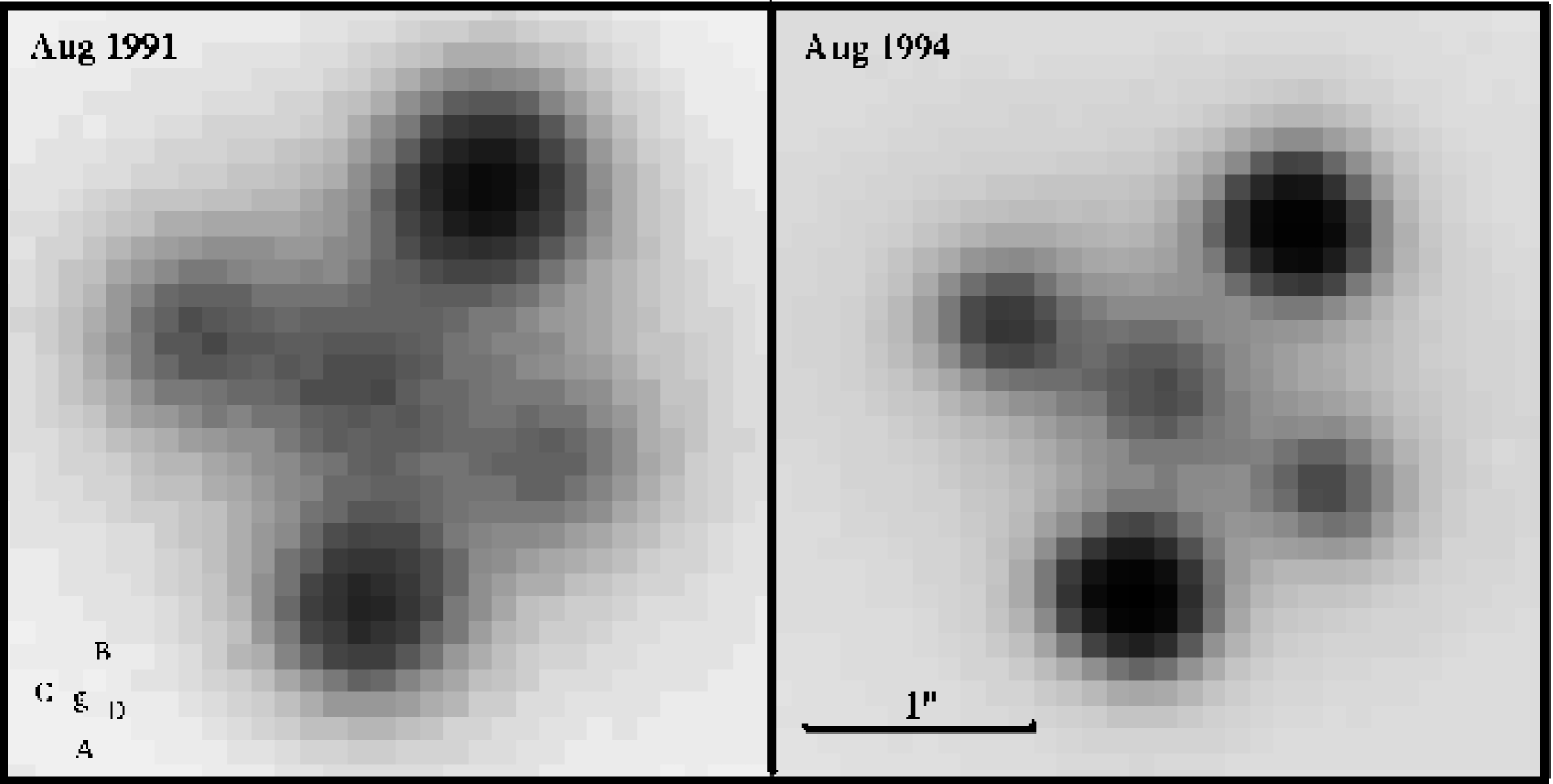
Figure 1: A grey–scale representation of the R–band WHT images of Q2237+0305 from the 1991 and 1994 epochs. The images have identical scales and orientations, and show a region $\sim 3\mbox{\mbox{${}^{\prime\prime}$}\hskip-3.00003pt.}25$ on a side with north to the top and east to the left. The legend in the lower left–hand corner of the August 1991 images shows the image designations of Yee (1988). Image A can be seen to have brightened substantially over the three year period.

3.2 Spectroscopy: Instrumental Configuration

The spectroscopic observations were acquired with the ISIS double–beam spectrograph [Clegg et al. 1992] at the Cassegrain focus of the WHT. On 1991 August 14 the spectrograph was configured with the $5400$ dichroic, splitting the red and blue beams at $\sim 5400$Å. The R158B grating in the blue arm combined with a thick $1152\times 1242$ pixel EEV CCD with 22.5${\rm\mu m}$ pixels produced a dispersion of 2.70 Å$/{\rm pixel}$. The grating angle was set to give a central wavelength of $\sim 4500$Å. The wavelength coverage in the blue is truncated at $\sim 3500$Å by the combined effects of atmospheric absorption and the rapidly falling sensitivity of the CCD, and in the red, at $\sim 5500$Å, by the dichroic cross–over wavelength. The R316R grating in the red arm combined with a second thick $1152\times 1242$ pixel EEV CCD with 22.5${\rm\mu m}$ pixels produced a dispersion of 1.40 Å$/{\rm pixel}$. The central wavelength was set at $\sim 7800$Å, giving a wavelength coverage $\lambda\lambda 7000$–$8600$Å. The spatial scale on the detector along the slit was $0\mbox{\mbox{${}^{\prime\prime}$}\hskip-3.00003pt.}335$/pixel for both red and blue arms.

The 1994 August 17 observations were obtained with a very similar instrumental configuration. Both red and blue gratings, central wavelengths and wavelength coverage were as for the 1991 observations. The $5700$ dichroic split the red and blue beams at $\sim 5700$Å, changing the wavelength coverage between the two arms slightly. The blue–arm detector had been upgraded to a $1024\times 1024$ pixel thinned TEK CCD with 24${\rm\mu m}$ pixels, decreasing the dispersion to 2.88 Å$/{\rm pixel}$ but producing much improved sensitivity. The spatial scale on the detectors along the slit was $0\mbox{\mbox{${}^{\prime\prime}$}\hskip-3.00003pt.}335$/pixel in the red arm and $0\mbox{\mbox{${}^{\prime\prime}$}\hskip-3.00003pt.}358$ in the blue arm.

Observations at both epochs therefore covered wavelengths $\lambda\lambda 3500-5400$ and $\lambda\lambda 7000-8600$, which, at the redshift of $z=1.69$ for Q2237+0305, include the prominent rest–frame emission lines of CIV $\lambda$1549, CIII] $\lambda$1909 and MgII $\lambda$2798 at wavelengths of $\sim 4175$Å, $5145$Å and $7540$Å, respectively. Unfortunately, the strong telluric absorption band at $\sim 7600$Å coincides with the red wing of the MgII emission line.

3.3 Spectroscopy: Observations

The atmospheric conditions during the spectroscopic observations at both epochs (1991 August 15 00:00-05:00UT and 1994 August 17 05:00-05:30UT), were excellent. The seeing derived from the spatial extent of the component quasar images was measured to be $\raisebox{-2.15277pt}{$\;\stackrel{{\scriptstyle<}}{{\scriptstyle\sim}}\;$}~{}0\mbox{\mbox{${}^{\prime\prime}$}\hskip-3.00003pt.}8$ at both epochs. A slit-width of $0\mbox{\mbox{${}^{\prime\prime}$}\hskip-3.00003pt.}70$ was used in 1991, producing spectral resolutions (FWHM of an unresolved arc line) of 8.1Å and 4.1Å in the blue and the red arms respectively. In 1994 a slit-width of $0\mbox{\mbox{${}^{\prime\prime}$}\hskip-3.00003pt.}91$ was employed giving spectral resolutions of 5.7Å,  and 4.1Å in the blue and the red arms respectively. Q2237+0305 was observed either side of the meridian with spectra obtained at airmasses of 1.1 to 1.4. The lower resolution in the blue–arm during the 1991 observations is probably a result of non–optimal spectrograph focus.

Spectra of pairs of images on the same side of the galaxy nucleus were obtained in order to minimize contamination from the galaxy core. Observations of sufficient pairs were acquired to ensure some redundancy in the observations of each component. The longer 1991 series comprised image pairs A+D, B+C, B+D, and A+C while the short sequence in 1994 (obtained as a Service allocation) comprised A+C and B+C. The four individual quasar images were clearly visible on the acquisition TV and the spectrograph slit, oriented to the appropriate position angle for the particular image pair, was aligned across each image pair using visual inspection. A log of the spectroscopic observations is given in Table 1. It was necessarily impossible to acquire the spectra of the image pairs with the spectrograph slit aligned along the parallactic angle. Differential atmospheric dispersion was thus expected to produce a systematic loss of light from the slit at the bluest wavelengths.

Year	Image Pair	Slit PA	Exposure	Airmass	Seeing
1991	A+D	302.8	1800	1.386	$0\mbox{\mbox{${}^{\prime\prime}$}\hskip-3.00003pt.}80$
1991	A+D	302.8	1800	1.254	$0\mbox{\mbox{${}^{\prime\prime}$}\hskip-3.00003pt.}80$
1991	B+C	290.8	1800	1.144	$0\mbox{\mbox{${}^{\prime\prime}$}\hskip-3.00003pt.}80$
1991	B+C	290.8	1800	1.125	$0\mbox{\mbox{${}^{\prime\prime}$}\hskip-3.00003pt.}80$
1991	B+D	8.8	1800	1.111	$0\mbox{\mbox{${}^{\prime\prime}$}\hskip-3.00003pt.}80$
1991	B+D	8.8	1800	1.134	$0\mbox{\mbox{${}^{\prime\prime}$}\hskip-3.00003pt.}80$
1991	A+C	27.8	1800	1.218	$0\mbox{\mbox{${}^{\prime\prime}$}\hskip-3.00003pt.}80$
1991	A+C	27.8	1800	1.316	$0\mbox{\mbox{${}^{\prime\prime}$}\hskip-3.00003pt.}80$
1994	A+C	27.8	1500	1.109	$0\mbox{\mbox{${}^{\prime\prime}$}\hskip-3.00003pt.}65$
1994	B+C	290.8	1500	1.108	$0\mbox{\mbox{${}^{\prime\prime}$}\hskip-3.00003pt.}65$

Table 1: Journal of spectroscopic observations of Q2237+0305 taken on the nights of 1991 August 14/15 and 1994 August 17/18.

Bias frames and exposures of quartz and tungsten lamps were obtained at the start of each night and flux standards [Massey et al. 1988, Oke 1990] were observed at the end of the night. Exposures of Cu+Ar (blue arm) and Cu+Ar/Cu+Ne (red arm) lamps were taken following each exposure of an image pair or a standard star.

4 Photometry

Figure 1 shows a grey–scale representation of the reduced R–band frames from the 1991 and 1994 epochs. Relative photometry of the individual quasar images was performed using the procedures described in Corrigan (1993). Exposures of standard stars were not obtained at either epoch and the frames were calibrated using stars visible both in frames from Corrigan (1993) and the new images. The uncertainty in the calibration is estimated to be $\pm 0.05\,$mag. R–band magnitudes for the four quasar images on the R–band system used in Corrigan et al (1991), are given in Table 2. The significant difference in the relative brightness of images A and B between the two epochs is evident from inspection of Figure 1, and the change in relative brightness, $\Delta m_{A-B}=0.38\pm 0.07\,$mag is well determined, independent of the calibration procedure.

Relative, and calibrated, magnitudes for the images at both epochs are consistent with the photometric time series (27 epochs) for the period 1990 to 1993, obtained by Østensen (1994) at the Nordic Optical Telescope, which shows image A brightening to become comparable to image B at the end of 1992.

	Seeing	A	B	C	D
1991	$0\mbox{\mbox{${}^{\prime\prime}$}\hskip-3.00003pt.}5$	17.53	17.23	18.11	18.28
1994	$0\mbox{\mbox{${}^{\prime\prime}$}\hskip-3.00003pt.}4$	17.12	17.20	18.00	18.23

Table 2: The R-band image magnitudes of Q2237+0305 at the 1991 and 1994 epochs. The errors in these measurements is 0.05 mag.

5 Spectroscopic Reductions

The relatively complex nature of the data, consisting of two merging quasar spectra superimposed upon an extended galaxy background, precluded the application of standard data reduction software to extract the spectra of the individual quasar components. A new reduction technique, therefore, was developed for application to this data. This technique is presented, in some detail, in Appendix A.

5.1 Spectral Fitting

The image separations, seeing and $\left<\chi^{2}\right>$, the average “goodness-of-fit” value (Appendix A.4), from the model–fitting procedure applied to the blue and red spectroscopic observations of each image pair are presented in Table 3. The seeing is defined as the FWHM of the Gaussian core of the profile model fitted to the two quasar spectra (Section A.3.1). For comparison, image separations derived from Hubble Space Telescope imaging of the system [Rix et al. 1992] are presented in Table 3.

We note that the red spectra in Table 3 possess systematically greater estimates of the width of the seeing profile when compared to the equivalent blue spectra. This may be due to an under–estimate of the galaxy component in the wings of the quasar profile, driving profile width to larger values. This, however, was not readily apparent in “by-eye” inspections of the fits as a function of wavelength. Such model dependencies will not effect the over–all conclusions presented in this paper.

		Blue Spectra			Red Spectra
Images	Year	$\Delta$	FWHM	$\left<\chi^{2}\right>$	$\Delta$	FWHM	$\left<\chi^{2}\right>$	$\Delta_{\rm HST}$
A+D	1991	$1\mbox{\mbox{${}^{\prime\prime}$}\hskip-3.00003pt.}07\pm 0\mbox{\mbox{${}^{\prime\prime}$}\hskip-3.00003pt.}25$	$1\mbox{\mbox{${}^{\prime\prime}$}\hskip-3.00003pt.}06\pm 0\mbox{\mbox{${}^{\prime\prime}$}\hskip-3.00003pt.}11$	1.23	$1\mbox{\mbox{${}^{\prime\prime}$}\hskip-3.00003pt.}07\pm 0\mbox{\mbox{${}^{\prime\prime}$}\hskip-3.00003pt.}23$	$1\mbox{\mbox{${}^{\prime\prime}$}\hskip-3.00003pt.}13\pm 0\mbox{\mbox{${}^{\prime\prime}$}\hskip-3.00003pt.}14$	1.91	$1\mbox{\mbox{${}^{\prime\prime}$}\hskip-3.00003pt.}01$
A+D	1991	$1\mbox{\mbox{${}^{\prime\prime}$}\hskip-3.00003pt.}09\pm 0\mbox{\mbox{${}^{\prime\prime}$}\hskip-3.00003pt.}26$	$0\mbox{\mbox{${}^{\prime\prime}$}\hskip-3.00003pt.}94\pm 0\mbox{\mbox{${}^{\prime\prime}$}\hskip-3.00003pt.}11$	1.29	$1\mbox{\mbox{${}^{\prime\prime}$}\hskip-3.00003pt.}05\pm 0\mbox{\mbox{${}^{\prime\prime}$}\hskip-3.00003pt.}24$	$1\mbox{\mbox{${}^{\prime\prime}$}\hskip-3.00003pt.}11\pm 0\mbox{\mbox{${}^{\prime\prime}$}\hskip-3.00003pt.}13$	1.91	$1\mbox{\mbox{${}^{\prime\prime}$}\hskip-3.00003pt.}01$
B+C	1991	$1\mbox{\mbox{${}^{\prime\prime}$}\hskip-3.00003pt.}38\pm 0\mbox{\mbox{${}^{\prime\prime}$}\hskip-3.00003pt.}22$	$0\mbox{\mbox{${}^{\prime\prime}$}\hskip-3.00003pt.}83\pm 0\mbox{\mbox{${}^{\prime\prime}$}\hskip-3.00003pt.}13$	1.34	$1\mbox{\mbox{${}^{\prime\prime}$}\hskip-3.00003pt.}44\pm 0\mbox{\mbox{${}^{\prime\prime}$}\hskip-3.00003pt.}19$	$1\mbox{\mbox{${}^{\prime\prime}$}\hskip-3.00003pt.}01\pm 0\mbox{\mbox{${}^{\prime\prime}$}\hskip-3.00003pt.}11$	1.48	$1\mbox{\mbox{${}^{\prime\prime}$}\hskip-3.00003pt.}39$
B+C	1991	$1\mbox{\mbox{${}^{\prime\prime}$}\hskip-3.00003pt.}36\pm 0\mbox{\mbox{${}^{\prime\prime}$}\hskip-3.00003pt.}25$	$0\mbox{\mbox{${}^{\prime\prime}$}\hskip-3.00003pt.}90\pm 0\mbox{\mbox{${}^{\prime\prime}$}\hskip-3.00003pt.}18$	1.40	$1\mbox{\mbox{${}^{\prime\prime}$}\hskip-3.00003pt.}42\pm 0\mbox{\mbox{${}^{\prime\prime}$}\hskip-3.00003pt.}22$	$1\mbox{\mbox{${}^{\prime\prime}$}\hskip-3.00003pt.}05\pm 0\mbox{\mbox{${}^{\prime\prime}$}\hskip-3.00003pt.}13$	1.74	$1\mbox{\mbox{${}^{\prime\prime}$}\hskip-3.00003pt.}39$
B+D	1991	$1\mbox{\mbox{${}^{\prime\prime}$}\hskip-3.00003pt.}23\pm 0\mbox{\mbox{${}^{\prime\prime}$}\hskip-3.00003pt.}27$	$0\mbox{\mbox{${}^{\prime\prime}$}\hskip-3.00003pt.}72\pm 0\mbox{\mbox{${}^{\prime\prime}$}\hskip-3.00003pt.}05$	1.21	$1\mbox{\mbox{${}^{\prime\prime}$}\hskip-3.00003pt.}21\pm 0\mbox{\mbox{${}^{\prime\prime}$}\hskip-3.00003pt.}30$	$1\mbox{\mbox{${}^{\prime\prime}$}\hskip-3.00003pt.}05\pm 0\mbox{\mbox{${}^{\prime\prime}$}\hskip-3.00003pt.}10$	1.77	$1\mbox{\mbox{${}^{\prime\prime}$}\hskip-3.00003pt.}18$
B+D	1991	$1\mbox{\mbox{${}^{\prime\prime}$}\hskip-3.00003pt.}20\pm 0\mbox{\mbox{${}^{\prime\prime}$}\hskip-3.00003pt.}31$	$0\mbox{\mbox{${}^{\prime\prime}$}\hskip-3.00003pt.}72\pm 0\mbox{\mbox{${}^{\prime\prime}$}\hskip-3.00003pt.}06$	1.25	-	-	-
A+C	1991	$1\mbox{\mbox{${}^{\prime\prime}$}\hskip-3.00003pt.}33\pm 0\mbox{\mbox{${}^{\prime\prime}$}\hskip-3.00003pt.}22$	$0\mbox{\mbox{${}^{\prime\prime}$}\hskip-3.00003pt.}84\pm 0\mbox{\mbox{${}^{\prime\prime}$}\hskip-3.00003pt.}14$	1.40	$1\mbox{\mbox{${}^{\prime\prime}$}\hskip-3.00003pt.}34\pm 0\mbox{\mbox{${}^{\prime\prime}$}\hskip-3.00003pt.}20$	$1\mbox{\mbox{${}^{\prime\prime}$}\hskip-3.00003pt.}12\pm 0\mbox{\mbox{${}^{\prime\prime}$}\hskip-3.00003pt.}13$	1.60	$1\mbox{\mbox{${}^{\prime\prime}$}\hskip-3.00003pt.}35$
A+C	1991	$1\mbox{\mbox{${}^{\prime\prime}$}\hskip-3.00003pt.}28\pm 0\mbox{\mbox{${}^{\prime\prime}$}\hskip-3.00003pt.}22$	$0\mbox{\mbox{${}^{\prime\prime}$}\hskip-3.00003pt.}89\pm 0\mbox{\mbox{${}^{\prime\prime}$}\hskip-3.00003pt.}11$	1.30	$1\mbox{\mbox{${}^{\prime\prime}$}\hskip-3.00003pt.}35\pm 0\mbox{\mbox{${}^{\prime\prime}$}\hskip-3.00003pt.}21$	$1\mbox{\mbox{${}^{\prime\prime}$}\hskip-3.00003pt.}17\pm 0\mbox{\mbox{${}^{\prime\prime}$}\hskip-3.00003pt.}13$	1.61	$1\mbox{\mbox{${}^{\prime\prime}$}\hskip-3.00003pt.}35$
A+C	1994	$1\mbox{\mbox{${}^{\prime\prime}$}\hskip-3.00003pt.}33\pm 0\mbox{\mbox{${}^{\prime\prime}$}\hskip-3.00003pt.}09$	$0\mbox{\mbox{${}^{\prime\prime}$}\hskip-3.00003pt.}57\pm 0\mbox{\mbox{${}^{\prime\prime}$}\hskip-3.00003pt.}03$	1.46	$1\mbox{\mbox{${}^{\prime\prime}$}\hskip-3.00003pt.}24\pm 0\mbox{\mbox{${}^{\prime\prime}$}\hskip-3.00003pt.}12$	$0\mbox{\mbox{${}^{\prime\prime}$}\hskip-3.00003pt.}99\pm 0\mbox{\mbox{${}^{\prime\prime}$}\hskip-3.00003pt.}05$	1.60	$1\mbox{\mbox{${}^{\prime\prime}$}\hskip-3.00003pt.}35$
B+C	1994	$1\mbox{\mbox{${}^{\prime\prime}$}\hskip-3.00003pt.}33\pm 0\mbox{\mbox{${}^{\prime\prime}$}\hskip-3.00003pt.}30$	$0\mbox{\mbox{${}^{\prime\prime}$}\hskip-3.00003pt.}79\pm 0\mbox{\mbox{${}^{\prime\prime}$}\hskip-3.00003pt.}10$	1.06	$1\mbox{\mbox{${}^{\prime\prime}$}\hskip-3.00003pt.}34\pm 0\mbox{\mbox{${}^{\prime\prime}$}\hskip-3.00003pt.}13$	$0\mbox{\mbox{${}^{\prime\prime}$}\hskip-3.00003pt.}90\pm 0\mbox{\mbox{${}^{\prime\prime}$}\hskip-3.00003pt.}08$	1.47	$1\mbox{\mbox{${}^{\prime\prime}$}\hskip-3.00003pt.}39$

Table 3: Spatial quantities (image separation and seeing) and average goodness–of–fit derived from the model–fitting to each of the blue and red spectroscopic observations. The one–sigma errors are derived from the total spectral fit. The final column presents the image separations, $\Delta_{\rm HST}$, from the HST observations of Rix et al.  (1992). The quoted error in the image positions as derived from HST imaging is $\mathrel{\mathchoice{\vbox{\offinterlineskip\halign{\hfil$\displaystyle#$\hfil\cr<\cr\sim\cr}}}{\vbox{\offinterlineskip\halign{\hfil$\textstyle#$\hfil\cr<\cr\sim\cr}}}{\vbox{\offinterlineskip\halign{\hfil$\scriptstyle#$\hfil\cr<\cr\sim\cr}}}{\vbox{\offinterlineskip\halign{\hfil$\scriptscriptstyle#$\hfil\cr<\cr\sim\cr}}}}0\mbox{\mbox{${}^{\prime\prime}$}\hskip-3.00003pt.}015$.

5.2 The Spectra

Figure 2: The four blue spectra of Image A obtained in 1991. The spectra have been corrected for the instrument response and normalized such that the mean flux in the continuum region 4400 $\rightarrow$ 4900Å is identical.

As an illustrative example of the extracted spectra, Figure 2 presents all four blue spectra of image A obtained in 1991. The spectra are normalized such that the average flux in the continuum region 4400 $\rightarrow$ 4900Å is the same. To within the noise, there is excellent agreement between the independent observations of the spectrum, with typical differences being $\sim 10\%$.

It should be noted that the spectra show no apparent distortion due to the effects of atmospheric dispersion. The A+D and A+C image pairs were observed at very similar zenith distances, but either side of the upper culmination. At these air masses the resulting slit orientations lay within $\sim 15^{o}$ of the parallactic angle, resulting similar atmospheric dispersion for each spectrum. This was not the case for the 1994 observations, both of which were observed very near the upper culmination. Atmospheric dispersion, coupled with a narrow slit and good seeing, produced significant loss of light at the blue end of the spectra.

5.3 Scaled Spectra

The narrow slits and the requirement to orient the position angle away from the parallactic, (Section 3), mean that spectra of the individual images cannot be compared using an absolute flux scale. However, the principal effect predicted to arise from differential microlensing of the continuum and emission line producing regions will manifest itself as differences in emission line equivalent–width among the spectra of the images.

Any such differences in equivalent–widths between the spectra should be evident visually if the spectra are scaled such that their continuum levels are coincident. Equivalent–width differences will then manifest themselves as emission line strength changes. Figures 3–6 show the 1991 epoch blue and red spectra of such continuum–scaled spectra for the image pairs, A+C, A+D, B+C and B+D respectively. The spectra are plotted following the multiplicative scaling of the fainter spectrum such that the mean fluxes in the “continuum” regions 4650 $\rightarrow$ 4900Å (in the blue), and 7000 $\rightarrow$ 7080Å in the red spectra are equal.

Spectra of the image pair A+B (Figure 3) show no obvious systematic difference in emission line strength. However, Figure 4 shows image D has significantly stronger emission lines than image A and similarly Figure 5 demonstrates that image C has stronger emission lines than image B. Consistency in the emission line strength differences between the images is demonstrated in Figure 6 where image D is seen to possess a very marked excess of emission compared to the spectrum of image B. In addition to the three prominent emission lines of CIV, CIII] and MgII, evidence for an excess at 4455Å, coincident with HeII $\lambda 1640$ is present.

Figure 3: The blue (left panel) and red (right panel) ISIS spectra for images ${\rm A+C}$ from the 1991 observations. In the top panels the spectrum of C has been scaled to match the spectrum of image A in the $\rm\left(4650\rightarrow 4900\AA\right)$ in the blue spectrum, and $\rm\left(7000\rightarrow 7080\AA\right)$ in the red spectrum. The brighter A image is presented as a thick line, where as the scaled C spectrum is a thin line. The lower panel presents the difference in these spectra, defined as the spectra of A minus the scaled spectrum of C.

Figure 4: As for Figure 3, presenting the spectra for image A and image D in 1991, which has been scaled so that the continua match. The thinner line represents the scaled spectrum of the D image, while the thicker line is for image A. The difference between these spectra, presented in the lower panels, is defined to be the spectrum of the A image subtracted from the scaled D spectrum.

5.4 Emission Line Equivalent Widths

The emission line equivalent width ($EW$) provides a quantitative measure of emission line strength:

$$EW=\int_{\lambda_{1}}^{\lambda_{2}}\frac{\left[S\left(\lambda\right)-I\left(\lambda\right)\right]}{I\left(\lambda\right)}\ \ d\lambda$$ (4)

where $S\left(\lambda\right)$ is the flux at wavelength $\lambda$and $I\left(\lambda\right)$ is the flux in the underlying continuum at a wavelength $\lambda$. Wavelengths, $\lambda_{1}$ and $\lambda_{2}$ are chosen to bound the line of interest.

Establishing the true continuum level in rest–frame ultraviolet spectra of quasars is difficult due to the presence of weak emission features [cf the composite quasar spectrum of Francis et al.  (1991)]. However, establishing the absolute equivalent width is not required, rather, a consistent measure of equivalent width that allows the relative emission line strength in the component spectra is all that is necessary. A continuum was estimated for each emission line based on the median flux within “continuum” bands on either side of the line. The continuum was set by the straight line connecting points defined by the median flux in each band at the mid–point of the wavelength range of each band. The EW was then calculated numerically according to Equation 4 with the summation extending from the long wavelength edge of the blue continuum band to the short wavelength edge of the red continuum band (Table 4). In the case of the MgII line the summation was truncated at 7590Å to avoid the strong telluric absorption feature at $\sim 7600$Å.

Line	$x_{l,1}$	$x_{l,2}$	$x_{u,1}$	$x_{u,2}$
CIV	3970	4040	4290	4300
CIII]	5020	5060	5220	5260
MgII	7450	7480	7700	7739

Table 4: For the emission lines, $x_{l}$ and $x_{u}$ represent the bounds on the regions used in the estimation of the continuum. The equivalent width is measured between $x_{l,2}$ and $x_{u,1}$, except for MgII where the summation was truncated at 7590Å to exclude the atmospheric A–band absorption.

Image	Year	CIV	CIII]	MgII
A	1991	$126.11\pm 1.52$	$43.73\pm 1.34$	$28.65\pm 0.96$
D	1991	$190.53\pm 4.35$	$61.28\pm 2.96$	$49.83\pm 1.92$
A	1991	$132.23\pm 1.72$	$38.78\pm 1.12$	$33.10\pm 0.92$
D	1991	$203.47\pm 5.08$	$64.02\pm 2.64$	$43.09\pm 1.72$
B	1991	$68.32\pm 0.65$	$20.91\pm 0.89$	$18.08\pm 0.53$
C	1991	$116.87\pm 2.06$	$47.23\pm 2.41$	$28.53\pm 1.18$
B	1991	$77.00\pm 0.61$	$25.66\pm 0.86$	$19.65\pm 0.55$
C	1991	$120.34\pm 1.93$	$45.66\pm 2.30$	$32.61\pm 1.17$
B	1991	$69.59\pm 0.68$	$28.96\pm 0.93$	$19.26\pm 0.64$
D	1991	$148.88\pm 2.65$	$83.12\pm 2.11$	$49.23\pm 1.92$
B	1991	$69.70\pm 0.84$	$29.03\pm 0.91$	-
D	1991	$179.62\pm 3.73$	$93.29\pm 3.31$	-
A	1991	$99.91\pm 1.03$	$40.61\pm 1.06$	$28.05\pm 0.73$
C	1991	$112.41\pm 2.12$	$36.92\pm 1.76$	$25.05\pm 1.16$
A	1991	$118.33\pm 1.33$	$38.20\pm 1.16$	$27.48\pm 0.77$
C	1991	$83.37\pm 2.20$	$37.45\pm 2.01$	$24.76\pm 1.29$
A	1994	$102.21\pm 0.43$	$36.44\pm 0.63$	$25.93\pm 0.46$
C	1994	$151.80\pm 1.60$	$51.73\pm 1.64$	$29.96\pm 0.94$
B	1994	$101.45\pm 1.12$	$30.51\pm 1.64$	$17.36\pm 0.58$
C	1994	$141.34\pm 3.18$	$45.51\pm 1.93$	$20.61\pm 1.10$

Table 5: Equivalent width measurements for images at both epochs. The error estimate is calculated assuming a continuum placement uncertainty of 2% for CIV and CIII, and a 5% error for MgII.

Image	Year	CIV	CIII]	MgII
A	1991	$119.14\pm 12.15$	$41.33\pm 3.80$	$29.32\pm 2.22$
B	1991	$71.15\pm 3.42$	$26.14\pm 3.31$	$19.00\pm 0.67$
C	1991	$108.33\pm 14.50$	$41.82\pm 4.67$	$27.74\pm 3.18$
D	1991	$180.63\pm 20.18$	$75.43\pm 13.31$	$47.38\pm 3.08$
A	1994	$102.21$	$36.44$	$25.93$
B	1994	$101.45$	$30.51$	$17.36$
C	1994	$146.57\pm 5.23$	$48.62\pm 3.11$	$25.28\pm 4.67$

Table 6: Mean values of the emission line equivalent widths from independent spectra. The $1\sigma$ errors represent the measured error in the mean. Only one spectrum of each of images A and B was obtained in 1994, and the errors in the values of the equivalent widths are assumed to be similar for those found for Image C.

Table 5 presents equivalent width measurements of CVI, CIII] and MgII for spectra taken in 1991 and 1994. The errors are calculated assuming an uncertainty in the continuum placement of 2% for CIV and CIII, and 5% for MgII. Mean equivalent widths for each image at each epoch are given in Table 6, together with the $1\sigma$ errors in the mean.

5.5 Emission Line Centroid Shifts

Nemiroff (1988) and Schneider and Wambsganss (1990) predicted that gravitational microlensing of substructure in the broad line emitting region would result in significant profile differences between the same emission line in different images. Selective microlensing enhancement of portions of the emission line region undergoing ordered rotation, or outflow, could result in shifts of $\sim 1000$km s^-1 in the central wavelengths of emission lines.

Any differences in emission line centroids can be quantified by cross–correlation. The cross–correlation between two discrete signals $\mu_{i}$ and $\nu_{j}$ is defined to be:

$$C(\mu,\nu)_{k}\equiv\sum_{j=0}^{N-1}\mu_{k+j}\nu_{j}.$$ (5)

Computation of the cross–correlation function using observed galaxy spectra and zero–redshift templates is a standard technique in establishing redshifts [Tonry and Davies 1979]. Here, emission lines in different images arising from the same transition were cross–correlated. The quasar continuum was first subtracted from each emission line using the continuum definition procedure employed to perform the measurement of the equivalent widths. Then, the pairs of continuum subtracted emission lines were cross–correlated using the Numerical Recipes CORREL routine [Press et al. 1988]. Due to the presence of the telluric A–band absorption, only the region blue–ward of 7590Å was used in the analysis of the MgII velocity characteristics.

A Gaussian function was fitted to the central portion of the resulting cross–correlation function in order to provide a measure of the peak location. The function took the form:

$$C(x)=Ae^{-\left(\frac{\left|x-x_{c}\right|}{c}\right)^{2d}}$$ (6)

where $x_{c}$ is the central position of the peak of the distribution of width $c$. $A$ is a normalization factor, and $d$ is a free parameter. The fitting algorithm was an implementation of the Levenberg-Marquardt minimization method, as presented by Press et al.  (1988) in MRQMIN. The peak–fitting was undertaken using apertures ranging from ten to eighty pixels either side of the peak. The location of the peak centre depended somewhat upon the aperture used, as the form of the cross–correlation peak is not perfectly represented by Equation 6 ie large apertures tended to fit the cross–correlation peak wings, while small apertures didn’t possess the curvature sufficient to accurately identify the peak. For these reasons various apertures were applied to each cross-correlation peak. This resulted in the selection of a separate aperture to to reproduce the form of each peak.

The sensitivity of the cross–correlation analysis with spectra of the signal–to–noise ratio available is approximately $50\>\mbox{\rm km~{}s\mbox{${}^{-1}$}}$ ($1\sigma$). The velocity shifts for any of the three emission lines between any of the image pairs were all consistent with no velocity offset. For each line in the 1991 data, the mean velocity was; $4.6\pm 20.9\>\mbox{\rm km~{}s\mbox{${}^{-1}$}}$ for CIV, $48.1\pm 88.9\>\mbox{\rm km~{}s\mbox{${}^{-1}$}}$ for CIII and $18.0\pm 27.3\>\mbox{\rm km~{}s\mbox{${}^{-1}$}}$ for MgII. The uncertainties quoted are $1\sigma$ and are based on the uncertainty of the peak–fitting procedure described above. No systematic offset was seen for any of the cross–correlation peaks and these values suggest that there are no significant differences in the central velocity of the lines.

Consideration was also given to whether emission line profile differences were present between images. Such differences are expected due to some preferential amplification of any substructure in the broad emission line region [Nemiroff 1988, Schneider and Wambsganss 1990]. However, the limited signal-to-noise ratio of the data precludes the derivation of astrophysically useful constraints on possible line shape differences.

6 Discussion

6.1 Quasar Emission Regions

Table 6 and the spectra shown in Section 5.3 demonstrate that during the 1991 observations, strong equivalent width differences existed between the spectra of the four images. This result is consistent with standard models of quasar structure, with the scale of the broad line emitting region significantly greater than that of the continuum source. Schemes, such as the star-burst model, where emission lines originate in narrow supernovae shells embedded in a large continuum emitting source [Cid-Fernandez 1995], cannot account for the systematic lack of enhancement of the line flux during microlensing.

Image	Year	CIV	CIII]	MgII	Year	CIV	CIII]	MgII
A	1991	1.10	0.99	1.06	1994	0.70	0.75	1.02
B	1991	0.66	0.63	0.68	1994	0.69	0.63	0.69
C	1991	1.00	1.00	1.00	1994	1.00	1.00	1.00
D	1991	1.67	1.80	1.71	-	-	-	-

Table 7: The equivalent widths for the images in Q2237+0305, normalized with respect to measurements for image C at each epoch.

Table 7 presents the equivalent widths from both epochs of observation, normalized with respect to the equivalent of each line in the spectrum of image C. During the 1991 observations image A had equivalent widths of order unity when compared to those of image C, while each value in image B was $\sim 0.65$ that of C. Image D, on the other had equivalent width measures of $\sim 1.7$ those of C, reflecting the microlensing deamplification of its continuum. This interpretation is consistent with recent observations which show image D to have a radio brightness which is comparable to the other images in this system [Falco et al. 1996]. The photometry of system at the two epochs illustrate that image A had brightened over the three years, becoming as bright as image B. This is reflected in the values of Table 7. Essentially, the equivalent widths of image B, relative to those of image C, are unchanged between 1991 and 1994, while image A, on the other hand, has shown a strong decrease in the line-to-continuum strength in both CIV and CIII]. The EW measurements can be explained if image A underwent a microlensing event between the two epochs. The measure of the MgII equivalent width in image A, relative to that of image C, does not change between the 1991 and 1994 observation. The reason for this constant value in MgII is still unknown.

The ratio of the equivalent widths presented in Table 7 indicate that, at the time of observation, the spectral slope of the quasar images was independent of the level of microlensing amplification, with an equal level of enhancement in the red and blue regions of the spectrum. In the rest frame of the quasar, the spectra presented here cover the range 1500Å to 2800Å, which, if one adopts a temperature structure of the form $T(R)\propto R^{-\frac{3}{8}}$ as appropriate for the inner, radiation–dominated region of an optically thick, geometrically thin accretion disk [Shakura and Sunyaev 1973], implies that

$$\frac{R_{{\rm 2800}}}{R_{\rm 1500}}\sim 5.$$ (7)

For the corresponding effective temperatures, these emission regions are $\mathrel{\mathchoice{\vbox{\offinterlineskip\halign{\hfil$\displaystyle#$\hfil\cr<\cr\sim\cr}}}{\vbox{\offinterlineskip\halign{\hfil$\textstyle#$\hfil\cr<\cr\sim\cr}}}{\vbox{\offinterlineskip\halign{\hfil$\scriptstyle#$\hfil\cr<\cr\sim\cr}}}{\vbox{\offinterlineskip\halign{\hfil$\scriptscriptstyle#$\hfil\cr<\cr\sim\cr}}}}10^{15}$cm in extent, both the red and blue light comes from a fraction of an Einstein radius (Equation 1), and light curves in both colours should exhibit similar properties. The difference in scale size will only be apparent as colour differences when a caustic passes over the source [Wambsganss and Paczyński 1991] and it is probable that all the sources lie in inter-caustic regions.

6.2 Structure in the Broad Line Region

To the limit of the sensitivity, $\sim 150\>\mbox{\rm km~{}s\mbox{${}^{-1}$}}$, no significant velocity differences between the same emission lines in the spectra of different images in the Q2237+0305 system were found. Thus, any substructure in the broad emission line region must be large enough to be insensitive to the effects of microlensing. With Equation 3, this implies substructure in the broad line region must be on scales $\mathrel{\mathchoice{\vbox{\offinterlineskip\halign{\hfil$\displaystyle#$\hfil\cr>\cr\sim\cr}}}{\vbox{\offinterlineskip\halign{\hfil$\textstyle#$\hfil\cr>\cr\sim\cr}}}{\vbox{\offinterlineskip\halign{\hfil$\scriptstyle#$\hfil\cr>\cr\sim\cr}}}{\vbox{\offinterlineskip\halign{\hfil$\scriptscriptstyle#$\hfil\cr>\cr\sim\cr}}}}0.05h_{\scriptscriptstyle{50}}^{\scriptscriptstyle{-\frac{1}{2}}}$ pc.

Figure 5: As for Figure 3, presenting the spectra for image B and image C in 1991, which has been scaled so that the continua match. In the top panels, the B image is represented by a thick line, whereas the scaled C image is a thin line. The difference between these spectra is presented in the lower panel and the spectrum of the B image subtracted from the scaled spectrum of the C image.

Figure 6: As for Figure 3, presenting the spectra for image B and image D in 1991, which has been scaled so that the continua match. In the upper panels, the B image is represented by a thick line, while the scaled D image is a thin line. Although the continua agree the relative flux in the emission lines is very different between the images. This is also apparent in the lower plots which presents the scaled D image minus the B image. The data red–ward of ${\rm 5350\AA}$ in the left–hand plot, and blue–ward of ${\rm 7400\AA}$ in the right–hand plot were neglected due to very poor signal in the D spectrum at these wavelengths.

Appendix A Spectroscopic Reductions

Figure 7: Upper panel, model–fit (solid line) including contributions from the quasar and galaxy components (dashed lines) and the data (heavy solid line). $\chi^{2}(\lambda_{j})=0.545$. In the wings, at Pixels$<86$ and Pixels$>98$ only the galaxy contributes to the model fit. The lower panel presents the residuals (data-model), in counts (solid line and left hand axis), and normalized by the noise (dashed line and right hand axis).

A.1 Initial Reductions

Bias subtraction and flat-fielding were accomplished using standard procedures within the IRAF reduction package. To accomplish sky subtraction, the sky level was estimated directly from the CCD frames by defining strips either side of the the quasar spectra. These strip were 15 pixels in extent, starting at least 30 pixels from the quasar spectra. At this distance the contribution of the extended galaxy is negligible. The average of the median values of the sky in each strip was adopted as the sky value at each wavelength increment. There was no evidence of a gradient in the sky along the slit. For each object–frame a companion error–frame, recording the noise per pixel – including contributions from sky and object counts, CCD read–noise and flat-fielding uncertainties – was retained.

Wavelength and flux calibration proved straightforward. Uncertainties in the wavelength calibration, derived from the residuals of individual arc lines about the cubic–spline fits employed were 0.2Å in the blue and 0.05Å in the red. Relative fluxes, to an accuracy of $\sim$10% across the spectra, were obtained following repeat observations of standard stars. Given the narrow slits used and the systematic loss of light due to atmospheric dispersion it was decided that the final spectra should not be flux calibrated.

Following sky subtraction, each CCD frame consisted of two quasar spectra superimposed upon the more extended lensing galaxy. Coefficients to perform wavelength and flux conversions were retained but not applied to the target frames, i.e. no rebinning or scaling that would compromise the independence of the noise from pixel to pixel was performed. The proximity of the quasar images to one–another, $\sim 1\mbox{\mbox{${}^{\prime\prime}$}\hskip-3.00003pt.}2$, and the presence of the galaxy light precluded the use of conventional extraction procedures. Instead, a procedure whereby the composite profile was modeled by three components, the two unresolved quasars and the galaxy, was employed.

A.2 Spectroscopic Extraction

Figure 8: Image centroids determined from the first stage of the fitting procedure and the analytic third–order polynomial representations which allow the centroids to be specified at each wavelength increment. The data is from the red spectrum of images A+C, taken in 1994.

The key to the effective application of a multi–component model fitting procedure to estimate the contributions of the two quasar components and the galaxy at each wavelength increment is to reduce the number of free parameters to a minimum. In principle, the number of free parameters is large as three object profiles, their locations along the slit and their relative heights all need to be determined. However, a significant reduction can be achieved by taking advantage of the well–behaved and slowly varying properties of the spectra as a function of wavelength.

Specifically, the centroids of the three components along the slit (pixel position on the Y–axis of the CCD frame) varies smoothly (see below) as a function of wavelength (pixel position on the X–axis of the CCD frame). An analytic fit to the location of the centroids of the components as a function of wavelength allows the three component centroid positions to be specified prior to the model fitting at each wavelength.

The profiles of the two (unresolved) quasars components are identical, reducing the number of independent profiles to be determined from three to two. Furthermore, the variation in profile–shape with wavelength, arising from the combined effects of the wavelength–dependent atmospheric seeing and scattering in the spectrograph, is well–behaved, allowing the shape of the quasar profiles to be specified at each wavelength increment.

Thus, implementation of the model–fitting procedure involves two stages: In the first, the systematic variation of the positions and shape of the component profiles is determined and the shape of the component profiles estimated. In the second stage the contributions of the three components, essentially the relative intensity of the three component profiles, at each wavelength (pixel) increment is calculated using a non–linear minimization routine.

In the first stage of the model–fitting procedure, an unweighted fit, neglecting any galaxy component, is used to establish the centroids of the point spread function of the quasar components. The location of the image centroids can then be represented by an analytic function, reducing the number of free parameters to three: the width of the seeing profile, and the normalization of each of the quasar components. The concluding stage of the procedure consists of a fully weighted model–fit, including a model for the galaxy contribution. Before considering the details of the quasar and galaxy profiles adopted, an overview of the entire procedure is provided. The analysis proceeds as follows:

1. An unweighted fit of a model consisting of two identical image profiles (the quasars) is undertaken for each wavelength increment in the CCD frame. Five free parameters, the profile centroids, the profile heights and the profile width (effective seeing) are determined via a Fortran90 implementation of a modified version of the AMEOBA algorithm of Press et al.  (1988). The initial location for the profile centroid (along the slit) is specified interactively for the first wavelength increment. For subsequent wavelengths, the location of the centroid from the previous wavelength increment is employed. The contribution from the galaxy profile is ignored at this stage. The unweighted fit is very sensitive to the peaks of the (quasar) point spread functions.

2. An analytic function is then fit to the resulting profile centroid positions with the constraint that the profile separation remains constant (independent of wavelength). A third order polynomial representation produces excellent results (Figure 8). The zeroth–order terms were allowed to differ, while higher–order terms were forced to match for each of the quasars.

3. A model fit, as in step (i) above, is then performed, but now variance–weighting is employed and the two image centroids derived from the polynomial representation determined in step (ii). Three free parameters are calculated, the profile width and the heights of the two quasar profiles.

4. An analytic function is then fit to the resulting profile width as a function of wavelength. As for the centroid positions the dependence of the profile width on wavelength is smooth and well behaved allowing a very accurate representation using a simple analytic function.

5. Finally, a variance–weighted model fit is employed with the image centroids and profile width determined from their respective analytic representations. There are only three parameters remaining, the heights of the two quasar profiles and the galaxy profile. The relative contributions of each component from the fit averaged over one CCD exposure are illustrated in Figure 7.

   An accurate representation of the quasar and galaxy profiles and a quantitative measure of goodness–of–fit between data and model are required for the model–fitting approach to work effectively.

A.3 Model Components

A.3.1 The Quasar Point Spread Functions

The very high signal–to–noise ratio spectra of the standard stars, obtained using the identical spectrograph configuration on the same night as the observations of Q2237+0305, were used to define the form of the point spread function (PSF) for unresolved point sources. An analytic function, $p(r)$, consisting of a Gaussian core with exponential wings described the point spread function to very high accuracy. $p(r)$ is defined:

$$p(r)=\left\{\begin{array}[]{ll}Ke^{-\frac{1}{2}\left(\frac{r}{\sigma}\right)^{2}}&{r<r_{lim}}\\ Pe^{-\frac{r}{\delta}}&{r>r_{lim}}\end{array}\right.,$$ (8)

where $r$ is the distance from the centre of the profile and $r_{lim}$ is the distance at which the two profiles join [Irwin 1985]. By ensuring that the profile is continuous in the zeroth and first derivatives at $r_{lim}$ then

$$P=\frac{K}{N}e^{2\log{N}},\quad\delta=\frac{\sigma}{\sqrt{2\log{N}}},$$ (9)

where $N$ is the fraction of the psf peak at which the profiles join. The condition that the profile is continuous in both the zeroth and first derivatives reduces the number of independent parameters to four; the central position, $x_{c}$; radial scale length, $\sigma$; normalization, $K$; and the join fraction, $N$.

Variations in atmospheric seeing produce changes in the PSF that are essentially confined to the central Gaussian core and the PSFs of all three standard star spectra could be modeled by fixing the join fraction, $N$ equal to $35\%$ of the peak profile intensity, thereby reducing the number of independent parameters necessary to describe the profile to three.

As described in the previous section, the centroid and width (the $\sigma$ parameter) of the quasar profiles as a function of wavelength are determined prior to the final stage of the model fitting. Thus the profile height, or normalization, is the sole parameter to be determined for each of the two quasar spectra.

A.3.2 The Galaxy Profile

The galaxy profile was modeled using a de Vaucoulers (1953) ${\rm r^{\frac{1}{4}}}$ profile. The core radius was chosen to $r_{e}=7\mbox{\mbox{${}^{\prime\prime}$}\hskip-3.00003pt.}0$, and the ellipticity to $\epsilon=0.31$, in accordance with the observation of Racine (1991). The profile was smoothed with a PSF of the form determined from the observations of the standard stars [Section A.3.1] with the profile width defined by the value calculated from the quasar spectra in the CCD frames. Virtual slits of $0\mbox{\mbox{${}^{\prime\prime}$}\hskip-3.00003pt.}7$ and $0\mbox{\mbox{${}^{\prime\prime}$}\hskip-3.00003pt.}91$ were defined across the resulting surface brightness distribution at the same orientation as the actual observations. The light distribution was integrated across the slit at high resolution along the slit to give the spatial profile of galaxy light observed through the slit. The profile could be well reproduced using an analytical model consisting of two Gaussian components and a constant DC level, and this analytic representation was employed in the model–fitting procedure, with the height of the galaxy model profile as the free parameter. The normalization of the galaxy component and the two quasar components are obtained simultaneously in the model–fitting procedure, thereby producing a galaxy spectrum in addition to the two quasar spectra. The galaxy spectrum extracted from one of the data frames, uncorrected for instrumental response, is presented in the right hand panel of Figure 9. For comparison, the spectrum of NGC 3379 [Kennicutt 1992], an E0 galaxy, redshifted to $(z=0.039)$ is shown in the left panel of the figure. The number of absorption features in common between the spectra, including CaII H&K $\lambda\lambda 3968,3934$, the $4000{\rm\AA}$ break, the G-band $\lambda 4300$, H$\delta$ $\lambda 4102$, H$\beta$ $\lambda 4861$, and MgI $\lambda\lambda 5173,5175$, indicates the success of the fitting procedure in recovering a spectrum with the absorption line properties expected to be present in the galaxy core.

Figure 9: The left panel shows a spectrum of NGC 3379, an E0 galaxy from the Kennicutt (1992) spectral atlas, redshifted to $z=0.039$, the redshift of the lensing galaxy in the 2237+0305 system. The right panel presents a galaxy spectrum extracted from the 1991 data for the B+D images. The spectrum has not been flux calibrated. A number of absorption features are common to both spectra, e.g.CaII H&K $\lambda\lambda 3968,3934$, the $4000{\rm\AA}$ break, the G-band $\lambda 4300$, H$\delta$ $\lambda 4102$, H$\beta$ $\lambda 4861$, and MgI $\lambda\lambda 5173,5175$.

A.4 Goodness–of–Fit

A standard $\chi^{2}(\lambda_{j})$ statistic was employed to ascertain the goodness–of–fit of the model to the data. The analysis procedure involves one–dimensional model fits, $M(\lambda_{j},y_{i})$, to the observed distribution counts, $S(\lambda_{j},y_{i})$, in the spatial direction at fixed wavelength, (i.e. index $\lambda_{j}$ is fixed).

$$\chi^{2}(\lambda_{j})=\frac{1}{N_{pix}}\sum_{i=1}^{N_{pix}}\ \frac{[S(\lambda_{j},y_{i})-M(\lambda_{j},y_{i})]^{2}}{\sigma^{2}(\lambda_{j},y_{i})},$$ (10)

where the model, $M(\lambda_{j},y_{i})$ is:

$$M(\lambda_{j},y_{i})=\int^{\scriptscriptstyle y_{i}+\frac{\Delta y}{2}}_{\scriptscriptstyle y_{i}-\frac{\Delta y}{2}}[Q_{1}(\lambda_{j},y^{\prime})+Q_{2}(\lambda_{j},y^{\prime})+G(\lambda_{j},y^{\prime})]dy^{\prime},$$ (11)

where $Q_{j}$ and $G$ are analytic models for the two quasar components and the galaxy respectively. These functions are integrated numerically over a pixel, where $\Delta y$ is the pixel width. The noise, $\sigma^{2}(\lambda_{j},y_{i})$, is:

$$\sigma^{2}(\lambda_{j},y_{i})=S(\lambda_{j},y_{i})+Sky(\lambda_{j})+R^{2},$$ (12)

where the first term represents the $\sqrt{N}$ noise from the quasar and galaxy components, the second component the $\sqrt{N}$ noise from the sky, and the third component the read noise, $R$, from the CCD.

The integrator used throughout was a Fortran90 implementation of the routine DQAG, a Gauss-Konrod general-purpose, globally adaptive integrator, available from the numerical mathematical software database GAMS . This integrator proved very capable in standard integral tests, especially with the polynomial type integrands utilized in the evaluation of the $\chi^{2}$ statistic.

Figure 10: Results of applying the analysis to the synthetic quasar data. Lower panel shows the determinations of the quasar image centroids. Middle panel presents the quasar profile width measures. Top panel shows the quasar spectra recovered. The solid line in each panel represents the input values.

Figure 11: The summed residuals from the model–fit to the synthetic data. Residuals (data-fit) in counts, in the spatial direction, averaged over the dispersion axis are shown as the solid line (left hand axis). The residuals, normalised by the noise at each pixel are shown as the dotted line (right hand axis).

A.5 Fitting Procedure Applied to Synthetic Data

To verify the effectiveness of the extraction technique, simulated observations, closely mimicking the properties of the actual data, were generated and the ability of the fitting procedure to recover the (known) input parameters tested. The two quasar components, utilizing the composite quasar spectra derived by Francis (1991), were represented by PSFs with peak heights of 60 and 120 counts, and profile width $\sigma=1$ pixel. The components were separated by 3.7 pixels, with one centroid at pixel position 98.15, while the second was placed at 101.85. The galaxy component had a peak height of 15 counts and the spatial profile of Section A.3.2. Poisson noise from the object, a sky noise of 6 counts, combined with a read noise $\sigma_{n}=10$ counts, were included. This resulted in a signal–to–noise ratio of $\sim$2.5–3.5 for the simulated quasar components, a value lower than the actual observations.

The results of the fitting procedure are illustrated in Figure 10. The lower panel presents the measured image centroids from the first stage of the fitting procedure. ${\rm P_{1}}$ and ${\rm P_{2}}$, are the mean positions and the $1\sigma$ scatter about the mean. The profile centroid separation is $3.69\pm 0.22$ pixels. The middle panel shows the recovery of the profile seeing width, $\sigma$. The top panel presents the individual spectra recovered by the analysis with the actual input spectra shown for comparison. Figure 11 presents the corresponding mean residual (solid line and left–hand axis) in the spatial direction. The dashed line represents the mean residual count normalized by the noise (right–hand axis) at each position. The residuals are small, typically $\mathrel{\mathchoice{\vbox{\offinterlineskip\halign{\hfil$\displaystyle#$\hfil\cr<\cr\sim\cr}}}{\vbox{\offinterlineskip\halign{\hfil$\textstyle#$\hfil\cr<\cr\sim\cr}}}{\vbox{\offinterlineskip\halign{\hfil$\scriptstyle#$\hfil\cr<\cr\sim\cr}}}{\vbox{\offinterlineskip\halign{\hfil$\scriptscriptstyle#$\hfil\cr<\cr\sim\cr}}}}15\%$, compared to the signal in the spectrum. The median value of the chi-squared merit function (Equation 10) over the fit is 1.20, a reasonable value considering the piece–wise and non–optimal nature of the fitting procedure.

Recovery of the two quasar components from an artificial data set with a signal–to–noise ratio and level of galaxy contamination closely matching that of the actual data gives confidence in the spectra obtained by applying the procedure to the observational data.

A.6 Robustness

Differences will occur between the models employed in the spectral fitting, namely the point spread function and the surface brightness distribution of the galaxy, and the true functions. Such differences can introduce systematic errors into the extracted quasar spectra, affecting quantities such as the emission line equivalent widths. However, the parameters employed in the modeling are derived from observations of the lensing system and standard stars, and such systematic errors should be small. These errors should, therefore, in no–way effect the overall conclusions of this paper.

References

- [Alcock et al 1996] Alcock, C. et al, 1996, Astrophys. J., 463, L67.
- [Blandford 1991] Blandford, R. D., 1991, Physics of Active Galactic Nuclei, Eds. Duschl, W. J. and Wagner, S. J..
- [Burbidge 1985] Burbidge, G., 1985, Astron. J., 90, 1399.
- [Chang and Refsdal 1979] Chang, K. and Refsdal, S, 1979, Nature, 282, 561.
- [Chang 1984] Chang, K., 1984, Astron. & Astrophys., 130, 157.
- [Cid-Fernandez 1995] Cid-Fernandez, R., 1995, Ph.D. Thesis, Cambridge.
- [Clegg et al. 1992] Clegg, R. E. S. et al., 1992, No. XXII: ISIS Astronomers’ Guide, Technical Report, La Palma.
- [Corrigan et al. 1991] Corrigan, R. T. et al., 1991, Astron. J., 102, 34.
- [Corrigan 1993] Corrigan, R. T., 1993, Ph.D. Thesis, University of Cambridge.
- [Crane et al 1991] Crane, P. et al, 1991, Astrophys. J., 369, 59.
- [Dar 1991] Dar, A., 1991, Nature, 353, 708.
- [de Vaucouleurs 1953] de Vaucouleurs, G., 1953, Astron. J., 58, 29.
- [Emmering et al. 1992] Emmering, R. T., Blandford, R. D. and Sholsman, I., 1992, Astrophys. J., 385, 460.
- [Falco et al. 1996] Falco, E. E., Perley, R. A., Wambsganss, J. and Gorenstein, M. V., 1996, Astron. J., 112, 897.
- [Filippenko 1989] Filippenko, A. V., 1989, Astrophys. J., 338, L49.
- [Filippenko 1991] Filippenko, A. V., 1991, Physics of Active Galactic Nuclei, Eds. Duschl, W. J. and Wagner, S. J..
- [Fitte and Adams 1994] Fitte, C. and Adams, G., 1994, Astron. and Astrophys., 282, 11.
- [Francis et al. 1991] Francis, P. J., 1991, Astrophys. J., 373, 465.
- [Grandi et al. 1992] Grandi, P. et al., 1992, Astrophys. J. Supp., 82, 599.
- [Houde and Racine 1994] Houde, M. and Racine, R., 1994, Astron. J., 107, 466.
- [Huchra et al. 1985] Huchra, J. et al., 1985, Astron. J., 90, 691.
- [Irwin 1985] Irwin, M. J., 1985, Mon. Not. Roy. ast. Soc., 214, 575.
- [Irwin et al. 1989] Irwin, M. J., Webster, R. L., Hewett, P. C., Corrigan, R. C. and Jedrzejewski, R. I., 1989, Astron. J., 98, 1989.
- [Jaroszyński et al. 1992] Jaroszyński, M., Wambsganss, J. and Paczyński, P. , 1992, Astrophys. J., 396, L65.
- [Jaroszyński et al. 1994] Jaroszyński, M. and Marck, J.-A., 1994, Astron. and Astrophys., 291, 731.
- [Kayser et al. 1986] Kayser, R., Refsdal, S. and Stabell, R., 1986, Astr. Astrophys., 166, 36.
- [Kennicutt 1992] Kennicutt, R. C., 1992, Astrophys. J. Supp., 79, 255.
- [Kent and Falco 1988] Kent, S. M. and Falco, E. E., 1988, Astron. J., 96, 1570.
- [Lewis et al. 1993] Lewis, G. F., Miralda-Escudé, J., Richardson, D. C. and Wambsganss, J., 1993, Mon. Not. R. astr. Soc., 261, 647.
- [Lewis and Irwin 1996] Lewis, G. F. and Irwin, M. J., 1996, Mon. Not. R. astr. Soc., 283, 225.
- [Massey et al. 1988] Massy, P., Strobel, K., Barnes, J. V. and Anderson, E., 1988, Astrophys. J., 328, 315.
- [Moffat 1969] Moffat, A., 1969, Astron. and Astrophys., 3, 455.
- [Nemiroff 1988] Nemiroff, R. J., 1988, Astrophys. J., 335, 593.
- [Oke 1990] Oke, J. B., 1990, Astron. J., 99, 1621.
- [Østensen 1994] Østensen, R. H., 1994, Ph.D. Thesis, University of Tromso.
- [Paczyński 1986] Paczyński, B., 1986, Astrophys. J., 301, 503.
- [Pen et al. 1994] Pen, U-L. et al., 1994, Gravitational Lenses in the Universe, Ed Surdej, J.
- [Press et al. 1988] Press, W. H. et al., 1988, Numerical Recipes: The Art of Scientific Computing, Cambridge University Press.
- [Pringle 1981] Pringle, J. E., 1981, Ann. Rev. Ast. and Ast., 19, 137.
- [Racine 1991] Racine, R., 1991, Astron. J., 102, 454.
- [Racine 1992] Racine, R., 1992, Astrophys. J., 395, L65.
- [Rauch and Blandford 1991] Rauch, K. and Blandford, R. D., 1991, Astrophys. J., 381, L39.
- [Rees 1984] Rees, M. J., 1984, Ann. Rev. Ast. and Ast., 22, 471.
- [Rees et al. 1989] Rees, M. J., Netzer, H. and Ferland, G. J., 1989, Astrophys. J., 347, 640.
- [Rix et al. 1992] Rix, H. W., Schneider, D. P. and Bachall, J. N., 1992, Astron. J., 104, 595.
- [Sanitt 1971] Sanitt, N., 1971, Nature, 234, 199.
- [Schmidt et al 1996] Schmidt, R., Webster, R. L. and Lewis, G. F., 1997, Mon. Not. Roy. ast. Soc., Submitted.
- [Schneider and Wambsganss 1990] Schneider, P. and Wambsganss, J., 1994, Astron. and Astrophys., 237, 42.
- [Schneider et al 1988] Schneider, D. P. et al, 1988, Astrophys. J., 294, 66.
- [Schneider et al. 1992] Schneider, P., Ehlers J. and Falco E. E., 1992, Gravitational Lenses, Springer-Verlag Press.
- [Saust 1994] Saust, A. B., 1994, Astrophys. J. Supp., 103, 33.
- [Shakura and Sunyaev 1973] Shakura, N. I. and Sunyaev, R. A., 1973, Astron. and Astrophys., 24, 337.
- [Tonry and Davies 1979] Tonry, J. and Davies, M., 1979, Astrophys. J., 84, 1511.
- [Turrel 1967] Turrel, J., 1967, Astrophys. J., 147, 827.
- [Tyson and Gorenstein 1985] Tyson, J. A. and Gorenstein, M. V., 1985, Sky & Tel., 70, 319.
- [Walsh et al. 1979] Walsh, D., and Carswell, R. F. and Weymann, R. J. , 1979, Nature, 279, 381.
- [Wambsganss 1990] Wambsganss, J., 1990, Gravitational Microlensing, Ph.D. Thesis, Mnchen.
- [Wambsganss et al. 1990] Wambsganss, J., Paczyński, B. and Schneider, P., 1990, Astrophys. J., 358, L3.
- [Wambsganss and Paczyński 1991] Wambsganss, J. and Paczyński, B., 1991, Astron. J., 102, 864.
- [Wambsganss 1992] Wambsganss, J., 1992, Astrophys. J., 392, 424.
- [Witt 1993] Witt, H.-J., 1993, Astrophys. J., 403, 530.
- [Webster et al. 1991] Webster, R. L., Ferguson, A. M. N., Corrigan, R. T. and Irwin, M. J., 1991, Astron. J., 102, 1939.
- [Yee 1988] Yee, H. K. C., 1988, Astron. J., 95, 1331.
- [Zurek et al. 1994] Zurek, W. H., Siemiginowska, A. and Stirling, S. A., 1994, Astrophys. J., 434, 46.