Microlensing of Broad Absorption Line Quasars

Abstract

The physical nature of the material responsible for the high–velocity, broad–absorption line features seen in a small fraction of quasar spectra has been the subject of debate since their discovery. This has been especially compounded by the lack of observational probes of the absorbing region. In this paper we examine the rôle of “microlenses” in external galaxies on observed variability in the profiles of broad absorption lines in multiply-imaged quasars. Utilizing realistic models for both the broad absorption line region and the action of an ensemble of microlensing masses, we demonstrate that stars at cosmological distances can provide an important probe of the physical state and structure of material at the heart of these complex systems. Applying these results to the macrolensed BAL quasar system, H1413+117, the observed spectral variations are readily reproduced, but without the fine–tuning requirements of earlier studies which employ more simplistic models.

1 Introduction

Microlensing in extragalactic systems has been seen not only to introduce rapid fluctuations into the light curves of macrolensed quasars [Irwin et al. 1989, Corrigan et al. 1991], but also to introduce significant variability into their spectral features [Filippenko 1989, Lewis et al. 1997]. Through the spectroscopic monitoring of such variations in microlensed quasars, the kinematics and scales of structure in their inner regions can be probed [Kayser et al. 1986, Nemiroff 1988, Schneider & Wambsganss 1990].

In this paper, the question of whether a peculiar class of quasars, those exhibiting Broad Absorption Line (BAL) features, can be microlensed in a similar fashion is addressed, and whether this microlensing can shed light on the physics of the material at the core of these quasars. A description of the background of the problem is presented, with reference to previous study. An outline of the simple, but realistic, model employed in this study is given and the action of microlensing at a fold caustic is described. The results of this study demonstrate that microlensing can provide a valuable probe of BAL quasars.

2 Background

2.1 Microlensing

Soon after the discovery of the first gravitationally lensed system [Walsh et al. 1979], Chang and Refsdal (1979) noted that the small–scale granularity in galactic matter distributions, the fact that galaxies are comprised of point–like stars rather than solely smoothly distributed material, would lead to a peculiar gravitational lensing effect. Although the image splitting by such stellar mass objects, $\left(\sim 10^{-6}\mbox{\mbox{${}^{\prime\prime}$}}\right)$, would be too small to be observable, the induced amplification by these “microlenses” could be substantial. As the degree of amplification is dependent upon the relative position of the source and microlensing star, individual stellar motions can introduce a significant time–dependent variability into the light curve of a distant source.

The original work of Chang and Refsdal (1979) considered the action of a single microlensing star on the light curve of a macrolensed quasar. The development of numerical techniques demonstrated that, with an ensemble of stars, the microlensing action combines in a highly non–linear fashion to introduce complex structure into a microlensed light curve [Young 1981, Paczyński 1986]. The implementation of the backwards ray–shooting technique [Kayser et al. 1986, Wambsganss 1990], and more recently the contour algorithm [Witt 1993, Lewis et al. 1993], allowed an analysis of the statistical properties of the microlensing induced variability (Lewis & Irwin 1995; 1996).

At the source, the microlensing scale length, the Einstein radius, for a solar mass star is given by [Schneider et al. 1992],

$$\eta_{o}=\sqrt{\frac{\rm 4GM_{\odot}}{\rm c^{2}}\frac{D_{ls}D_{os}}{D_{ol}}}\ ,$$ (1)

Here, $D_{ij}$ are the angular diameter distances between an observer (o), lens (l) and source (s), respectively. For typical multiply imaged quasars this characteristic scale is $\sim 0.01-0.1$pc.

Numerical simulations demonstrated that, at even low optical depths, the induced variability of a microlensed source can be extremely complex. This is due to the microlensing amplification possessing a strong dependence on the relative positions of the source quasar and microlensing stars which results in a similarly complex map of amplification over the source plane [Wambsganss 1990]. This map possesses an intricate web of lines of formally infinite amplification which are known as caustics. As these cross an extended source, dramatic flux variations can be observed [Chang 1984]. In the absence of a stellar velocity dispersion [Schramm et al. 1993, Wambsganss & Kundić 1995], the characteristic caustic crossing–time of a source is

$$\tau\sim\frac{f_{\rm 15}}{1+z_{l}}\frac{D_{ol}}{D_{os}}\frac{h_{75}}{v_{300}}yrs,$$ (2)

where the scale–size of the source is $f_{\rm 15}\times 10^{15}~{}{\rm h_{75}}$cm and $z_{l}$ is the redshift of the lensing galaxy [Kayser et al. 1986]. The velocity of the microlensing stars across the line–of–sight is 300$v_{300}$km s^-1. In observed macrolensed systems, $\tau\sim$ several months.

2.2 BAL Quasars^¶

BAL quasars, representing 3-10% of the quasar population, are identified as possessing spectra with resonance absorption line systems due to highly ionized species. Although associated with the source quasar, these lines exhibit bulk outflow velocities of 5000–30000 ${\rm km\;s^{-1}}$ [Turnshek 1984].

Several recent reviews have discussed the nature of these absorption line systems [Turnshek 1988, Turnshek 1995, Weymann 1995]. The following is drawn from these articles. Current theories present two possible models for the rarity of BAL quasars: the BAL covering fraction is close to unity such that all lines of sight would result in BAL systems, with only 3-10% of quasars possessing a BAL region, or, BAL absorption systems are ubiquitous, although the covering factor is small, equivalent to the percentage of quasars observed with BALs, therefore making the detection of BALs dependent upon the line of sight to the quasar core. However, it has been proposed that the size of the BAL covering factor could differ between individual quasars, resulting in differences of the observed BAL profiles.

Although the geometry of the BAL region has not been clearly defined through observations, polarization measurements and inferred electron densities have placed constraints on the scale–size of the BAL region. Namely, the region must lie within 30–500 pc from the central continuum source over the broad range of quasar luminosities. There is also evidence to suggest that the large scale geometry represents a disk, while locally, the individual clouds are confined to flat disk-like shapes whose surfaces are perpendicular to the plane of the entire disk [Turnshek 1986]. Column density measurements yield a radial extent of $\sim 10^{11}-10^{13.5}\rm{cm}$ for these clouds [Turnshek 1995, Murray et al. 1995], although scale lengths as small as $10^{8}$cm have been suggested [Weymann 1995].

Until recently, all observed BAL quasars have been classified as weak radio sources, suggesting that these and radio-loud quasars are drawn from mutually exclusive populations. However, Becker et al. (1997) recently identified the first known radio-loud BAL quasar. Lacking the typically strong characteristic quasar emission lines, this object possesses nearly saturated BALs, and a highly absorbed continuum, suggesting that the radio luminosity is possibly related to the degree of absorption to the object.

Observations have revealed that BAL quasars are more highly polarized than radio quiet non-BAL quasars [Moore & Stockman 1984]. It has been suggested that in BAL quasars, the continuum flux is attenuated upon leaving the continuum source as it passes through a broad emission line (BEL) region, a BAL region, or a scattering region [Goodrich & Miller 1995]. Higher polarized flux is due to scattering farther from the BEL clouds [Goodrich & Miller 1995, Goodrich 1997]. A recent polarization study [Ogle 1997] suggests that several different geometries of the distribution of BAL material could account for the polarization observed in several BAL quasar spectra, and that an equatorial outflow within the BAL region is the most probable case.

Many models attempt to explain the origin and confinement of the BAL region material: such as magnetically confined clouds [Arav et al. 1994] and x-ray–shielded flows [Murray et al. 1995]. The small distances from the central continuum source, coupled with high outflow velocities, imply short time–scales for the crossing of the individual clouds through the entire BAL region, as compared with the quasar lifetime. The constant source of the material which is necessary to maintain the BAL region could originate from several sources; including atmospheres of giant stars [Scoville & Norman 1995], novae [Shields 1996], parts of an inner obscuring torus, or parts of the accretion disk [Murray et al. 1995].

2.3 H1413+117

Serendipitously discovered in a survey of highly luminous quasars, H1413+117 consists of four images of a $z=2.55$ quasar, arranged in a cruciform with angular separations of $0\mbox{\mbox{${}^{\prime\prime}$}\hskip-3.00003pt.}77$ to $1\mbox{\mbox{${}^{\prime\prime}$}\hskip-3.00003pt.}36$ [Magain et al. 1988]. Although no individual lensing candidate has been identified in deep imaging [Lawrence 1996], Magain et al. (1988) noted that a number of absorption systems, at $z\sim 1.4-2.1$, could indicate the presence of several lensing candidates. This is borne out with the recent study of Kneib et al. (1997) who detected the presence of a “cluster” in front of H1413+117 in HST WFPC2 images, which they associate with these absorption systems. With the addition of CO observations [Barvainis et al. 1994, Barvainis et al. 1997, Yun et al. 1997] and the existence of the foreground cluster, Kneib et al. (1997) attempt to improve previous lensing models [Kayser et al. 1990]. This additional cluster potential, coupled with a modest mass lensing galaxy, is seen to accurately reproduce the observed system.

Spectroscopic observations of H1413+117 were undertaken by Angonin et al. (1990). As well as confirming the BAL nature of the source, it was noted that differences existed between the spectra of the individual images. Most noticeably, the relative strengths of the Si IV $\lambda\lambda 1394,1403$ and C IV $\lambda 1549$ emission lines vary between the images [Hutsemékers 1993], a signature of differential amplification due to microlensing by stellar mass objects [Sanitt 1971, Lewis et al. 1997]. Coupled with this, it was seen that in one of the images the associated BAL profiles exhibit significant differences of $\sim 20\%$ when compared to the other images.

Motivated by the BAL profile differences in the spectra of H1413+117, Hutsemékers (1993, Hutsemékers et al. 1994) undertook an investigation of the possible microlensing effects of stars on BAL profiles. This work examines the effects on an individual cloud, a sub-region with differing optical depth from the average of the entire BAL region, due to a single microlens.

Considering an isolated point mass microlens [Einstein 1936], Hutsemékers (1993) shows that the maximum resultant amplification is less than that of the observed spectral differences. The Chang-Refsdal lens (Chang & Refsdal 1979; 1984) considers the non-linear microlensing effects of a point mass located in a galactic shear, whereby critical curves and caustics will dictate the amplification effects. This model is able to reproduce the amplification seen within the spectra of the multiple images of H1413+117 [Hutsemékers 1993].

It was concluded that the observed spectral variations in the BAL profiles of H1413+117 could be a result of the selective magnification due to microlensing, but only for a specific, “fine-tuned” configuration; the cloud must be at the border of the BAL region and lie along a caustic, while the remainder of the BAL region must lie in an area of strong de-magnification. This model relies strongly on the distance between the projected center of the lens and the center of the BAL region; a slight change will greatly effect the resulting magnification of the region [Hutsemékers 1993].

3 A Model for the BAL Region

For the analysis presented here the quasar continuum source was modeled as a 2–dimensional Gaussian surface–brightness of radius $10^{15}~{}{\rm h_{75}^{-1}~{}cm}$ [Rees 1984]. The material producing the BAL absorption is placed along the line-of–sight to the continuum source and the surface–brightness of this source as viewed through this region, as a function of wavelength, was calculated.

Figure 1: The adopted profile of the Broad Absorption Line, as given by Equation (3). The parameters of this profile were chosen to represent absorption by C IV $\lambda 1549$.

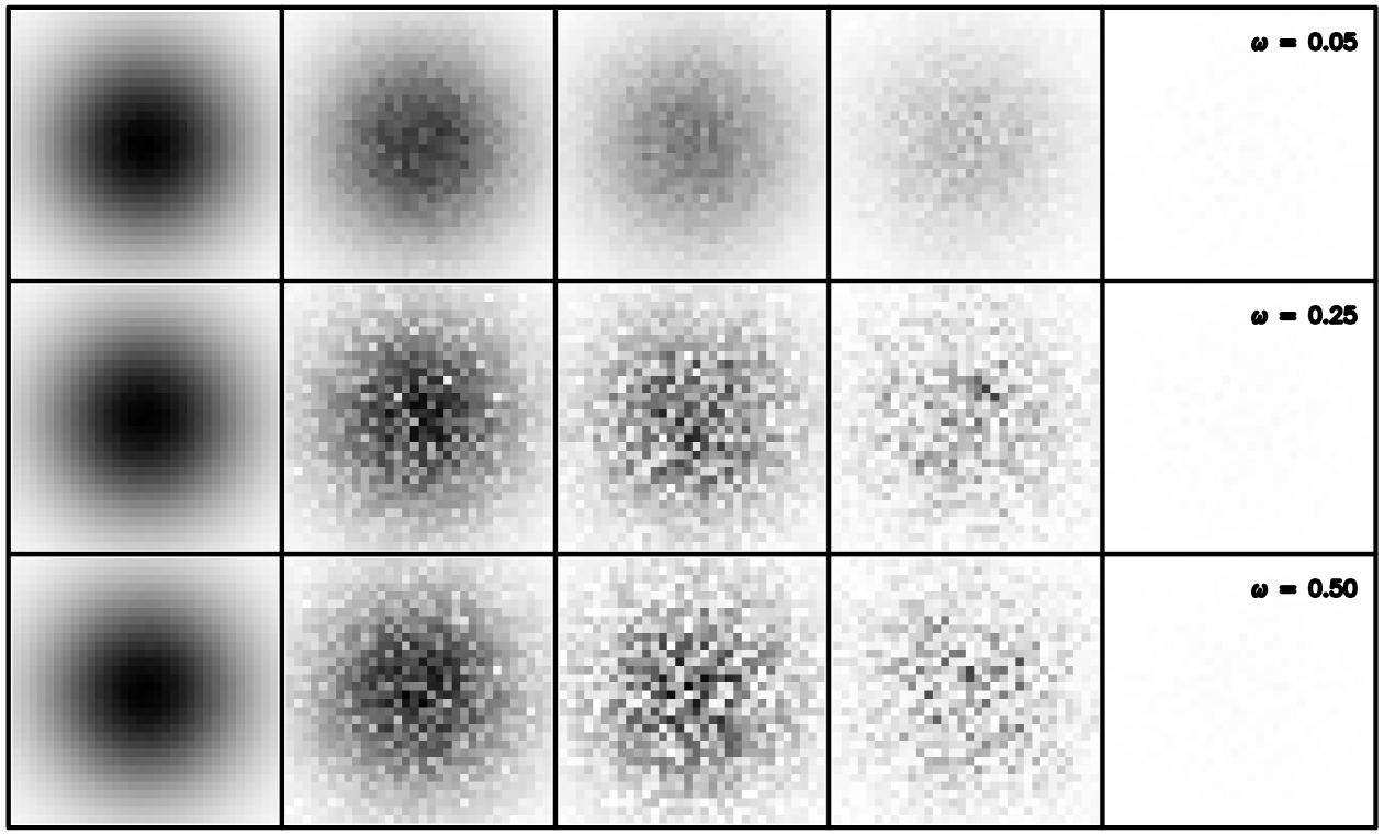
Figure 2: Running from left–to–right, these panels show the quasar continuum source at $1\%$, $25\%$, $50\%$, $75\%$ and $99\%$ absorption, respectively. From top–to–bottom, the panels represent absorption widths of $\omega=5\%$, $25\%$ & $50\%$, respectively. In this example, the absorption clouds are $1.2\times 10^{14}{\rm h_{75}^{-1}cm}$ in extent, while the entire source region is $3.7\times 10^{15}{\rm h_{75}^{-1}cm}$.

The absorption profile of the material within the BAL region was modeled with a simple functional form, namely

$${\rm A}\left(\lambda\right)=\frac{1}{1+\exp{\frac{\lambda-\lambda_{c}}{\Delta\lambda}}}$$ (3)

where $\lambda_{c}$ is the wavelength at which $50\%$ of the light from the continuum core is absorbed, while $2\Delta\lambda$ is the “width” of the absorption feature between $73\%$ and $27\%$ absorption. The absorption profile was chosen to represent the blue–wing of C IV $\lambda 1549$, with $\lambda_{c}=1505{\rm\AA}$, corresponding to a bulk outflow at $50\%$ absorption of $\sim 8500~{}{\rm km~{}s^{-1}}$. With an absorption width of $2~{}\Delta\lambda=8.75{\rm\AA}$, the resulting profile [Figure (1)] adequately represents observed C IV $\lambda 1549$ BAL profiles [Turnshek 1995, Weymann 1995].

The over–all BAL region is characterised by two quantities; a linear measure describing the scale–length of inhomogeneities in the absorbing material (henceforth referred to as the “cloud–size”), and the degree of variation of absorption at a particular wavelength. The distribution in absorption is represented by a Gaussian of width $\omega$, between 0% and 100% absorption, centred at $A_{c}\left(\lambda\right)$. This value was chosen such that the mean absorption, $\left<A\left(\lambda\right)\right>$, drawn from this distribution is the value given by Equation 3. Note that if, for a particular $\left<A\left(\lambda\right)\right>$ and $\omega$, that $A_{c}\left(\lambda\right)$ lies outside the 0% $\rightarrow$ 100% boundary, then $A_{c}\left(\lambda\right)$ is fixed at the boundary position and $\omega$ is varied to ensure $\left<A\left(\lambda\right)\right>$ follows Equation 3.

For this study we select the observational parameters of the quadruply lensed quasar H1413+117 [Angonin et al. 1990], with the source quasar being at $z=2.55$. Although the redshift of the lensing galaxy has yet to be established, there is evidence to suggest it is $z\sim 1.55$. This value is adopted here, resulting in an Einstein radius in the source plane, for a solar mass star, (Equation 1) of $1.9\times 10^{16}{\rm h_{75}^{-\frac{1}{2}}}$cm (Throughout we assume $\Omega=1$ and $\Lambda=0$).

Figure (2) presents an example of a quasar source as observed through the BAL region absorption clouds. The “source region”, $r_{s}$, is 3.7 source radii in extent and the clouds are laid out on a $32\times 32$ grid with a resulting scale–size of $1.2\times 10^{14}~{}{\rm h_{75}^{-1}~{}cm}$. From left–to–right the panels present absorption of 1%, 25%, 50%, 75% and 99% absorption, while from top–to–bottom $\omega$ = 5%, 25% and 50% respectively.

For the analysis presented here, we chose cloud sizes of $2^{-n}r_{s},n=1..9$. With this, the largest clouds were $1.8\times 10^{15}{\rm h_{75}^{-1}~{}cm}$ in extent while the smallest were $7.1\times 10^{12}{\rm h_{75}^{-1}~{}cm}$.

4 Microlensing Model

4.1 Amplification at fold caustics

At low to medium optical depths the scale of the BAL region is small compared to the typical scales of caustics produced by microlensing. Within this regime it can be assumed that the majority of caustics crossing the BAL source will be isolated fold catastrophes [Schneider et al. 1992]. Also, as the scale of the BAL source is expected to be much less than the caustic curvature it can be assumed that within the region of interest the caustic is locally straight. With this, the amplification of a point source at $y$, relative to a straight fold caustic at $y_{c}$ is given by 

$$\mu_{p}(y)=\sqrt{\frac{g}{y-y_{c}}}H(y-y_{c})+\mu_{o}.$$ (4)

Here, $y-y_{c}$ is the perpendicular distance between the point of interest and the caustic line, $H(y)$ is the Heaviside step function and $\mu_{o}$ is the amplification due to all other images of the source. This is assumed to be constant in the vicinity of the caustic. The parameter $g$ represents the “strength” of the caustic.

The amplification, or magnification, of an extended source is given by

$$\mu=\frac{\int\!\!\int I({\bf y})\,\mu_{p}({\bf y})\,d^{2}y}{\int\!\!\int I({\bf y})\,d^{2}y},$$ (5)

where $I({\bf y})$ is the surface brightness distribution of the source. If the source is considered to be a square “pixel” of uniform surface brightness which is aligned such that its sides are parallel/perpendicular to the caustic line, and it has its nearest edge a distance $y_{k}$ from a caustic of strength $g$, it will be magnified by a factor

$$\mu_{pix}=2\frac{\sqrt{g}}{\Delta y}\left(\sqrt{y_{k}+\Delta y}-\sqrt{y_{k}}\right)+\mu_{o},$$ (6)

where $\Delta y$ is the length of the side perpendicular to the fold caustic. Throughout $\mu_{o}=1$.

The “strength” of the caustic, $g$, was determined from a numerical study undertaken by Witt (1990). In this study, the parameter $\hat{K}=\sqrt{g}$, and, choosing a medium microlensing optical depth $(\sigma\sim 0.2)$, $\hat{K}$ was chosen to be 0.1, 0.4, 0.7, and 1.0. These values are representative of the broad distribution in caustic strengths found at such median optical depths.

For these various “strengths”, the caustic was swept across the source and the resultant flux, as a function of wavelength, was calculated. The resulting spectrum was normalized to the flux of the amplified unattenuated continuum. With this, the microlensed and intrinsic form of the BAL profile could be compared.

5 Results

Cloud Size	$\hat{K}=0.1$					$\hat{K}=0.4$
$2^{-n}$	5%	15%	25%	50%		5%	15%	25%	50%
1	2.14	5.56	6.46	11.02		4.65	12.07	14.06	23.95
2	1.17	3.11	7.39	5.37		2.54	8.63	16.07	11.81
3	0.93	2.35	3.88	4.18		2.23	5.63	9.33	10.03
4	0.55	1.32	2.05	2.12		1.20	3.10	4.64	5.11
5	0.29	0.82	1.15	1.72		0.65	1.87	2.84	3.91
6	0.16	0.49	0.74	0.76		0.38	1.14	1.68	1.90
7	0.09	0.24	0.36	0.51		0.23	0.61	0.87	1.06
8	0.05	0.16	0.25	0.23		0.12	0.38	0.53	0.58
9	0.03	—	0.11	0.15		0.08	—	0.26	0.34
Cloud Size	$\hat{K}=0.7$					$\hat{K}=1.0$
$2^{-n}$	5%	15%	25%	50%		5%	15%	25%	50%
1	5.59	14.50	16.91	28.77		6.08	15.76	18.40	31.29
2	3.33	11.57	19.31	15.84		3.85	13.40	21.56	18.34
3	2.78	7.20	11.67	12.55		3.09	8.34	12.96	14.29
4	1.44	4.25	5.82	6.49		1.67	5.08	6.47	7.81
5	0.79	2.31	3.60	4.78		1.03	2.60	4.04	5.25
6	0.50	1.42	2.11	2.48		0.58	1.70	2.39	2.81
7	0.30	0.81	1.09	1.25		0.33	0.92	1.24	1.37
8	0.16	0.48	0.63	0.74		0.18	0.54	0.68	0.84
9	0.10	—	0.34	0.44		0.11	—	0.39	0.50

Table 1: Maximum deviations in the lensed absorption spectra for four caustic strengths, $\hat{K}=0.1$, 0.4, 0.7, and 1.0, and four absorption dispersions, $\omega=5\%$, $15\%$, $25\%$, and $50\%$. The cloud size is represented as $2^{-n}r_{s},n=1..9$, where $r_{s}=3.7$ source radii, or $3.7\times 10^{15}{\rm h_{75}^{-1}cm}$, and ranges from $7.1\times 10^{12}{\rm h_{75}^{-1}cm}-1.8\times 10^{15}{\rm h_{75}^{-1}cm}$ in extent. The deviations are given as percentages of the normalized continuum flux, while the absorption dispersions are percentages of total absorption (see Section 3).

Cloud Size	Absorption Dispersion ($\omega$)
$2^{-n}$	15%	20%	25%	30%	40%
1	15.76	16.75	18.40	18.43	27.48
2	13.40	17.60	21.56	19.01	24.94
3	8.34	10.64	12.96	12.57	15.97
4	5.08	6.45	6.47	6.64	8.62
5	2.60	3.70	4.04	4.55	—

Table 2: Maximum deviations for caustic strength $\hat{K}=1.0$ and varying absorption dispersions ($\omega$). Cloud size is given as $2^{-n}r_{s},n=1..5$ (see Table 1), deviations are given as a percentage of the normalized continuum flux, and the absorption dispersion is the percentage of total absorption (see Section 3).

As the caustic line sweeps across the source, the magnification of the flux as seen through each “cloud” is calculated using Equation 6 and summed to give the total flux as a function of wavelength. As the entire flux from the region is amplified, the microlensed spectra are renormalized such that the continuum flux is one. The results of this analysis are summarized in Table 1, which presents the maximum flux deviations (as a percentage of the normalized continuum flux) between the unlensed spectra and lensed spectra. For large clouds, significant deviations from the unlensed form of the BAL profile can be seen, with these differences increasing with the caustic strength, $\hat{K}$, and the dispersion in the absorption, $\omega$.

Importantly, the degree of deviation is strongly dependent on the cloud size, with small clouds producing the smallest deviations, even with significantly inhomogeneous absorption distributions $(\omega=50\%)$. In this regime even the high amplification of an individual cloud is washed out in the overall amplification of the region. For such cloud distributions the BAL absorption region is essentially seen as smooth.

The solid line in Figure (3) presents an example of a microlensed BAL spectrum, while the dashed line represents the unlensed form of the BAL profile. As can be seen, there is significant deviations of the microlensed spectrum from the unlensed source ($\sim 30\%$). This is of similar order to the deviations observed in the spectra of H1413+117 [see Figure (1) in Hutsemékers (1993)]. In this case, the absorption clouds are $1.8\times 10^{15}{\rm h_{75}^{-1}cm}$ in extent ($2^{-1}r_{s}$), with an absorption dispersion $\omega=50\%$, while the lensing caustic is given a strength of $\hat{K}=1.0$.

Figure 3: The lensed absorption spectrum of a source with a cloud size of $1.8\times 10^{15}{\rm h_{75}^{-1}cm}$ ($2^{-1}r_{s}$), an absorption dispersion $\omega=50\%$, and a lensing caustic strength $\hat{K}=1.0$. The solid line represents the lensed spectrum at its maximum deviation of 31% (see Table 1) from the unlensed spectrum (dashed line). Each pixel has a velocity resolution of $\sim 200km\;s^{-1}$.

Figure (4) presents a typical amplification curve, demonstrating the temporal nature of variations. The cloud size in this simulation is $5.7\times 10^{13}{\rm h_{75}^{-1}cm}$ ($2^{-6}r_{s}$), with an absorption dispersion of $\omega=50\%$, while the caustic had a strength $\hat{K}=1.0$. The solid line presents the maximum deviation, at any wavelength, between the normalized microlensed spectrum and the unlensed profile, expressed as the absolute deviation from the continuum flux. The dashed line similarly presents the average absolute deviation as the caustic sweeps across the source. The degree of the deviation is strongly dependent on the the total amplification of the source, being zero before the caustic crosses, and tending again to zero after the caustic has passed.

Figure 4: A typical magnification curve for a lensed source with absorption clouds of $5.7\times 10^{13}{\rm h_{75}^{-1}cm}$ ($2^{-6}r_{s}$), $\omega=50\%$, and $\hat{K}=1.0$. The solid line represents the maximum deviation of lensed from unlensed source at each step of the caustic across the source. The dashed line is the average deviation as the caustic sweeps across the source. As the passage of the caustic over the source is reversible, these loops can be followed around either way.

As the cloud size approaches and becomes larger than the continuum region itself, the distribution of the absorbing material in front of the quasar becomes homogeneous. Such a scenario would not result in any flux deviations as the caustic sweeps over the source. We therefore would expect a turnover in the degree of fluctuations as the cloud size approaches this limit. To test this, additional simulations were undertaken for a fixed caustic strength, $\hat{K}=1.0$, varying absorption dispersions, $\omega=15\%$, $20\%$, $25\%$, $30\%$, and $40\%$, and cloud sizes of $2^{-n}r_{s},n=1..5$. Results of this are summarized in Table 2. This turnover is not apparent for small absorption dispersions, but is seen for medium absorption values. The turnover again vanishes for large absorption dispersions. This could be a result of the variation of $\omega$ (see Section 3) at the extreme ends of the BAL profile. For these absorption dispersions, $\omega$ is constant for the range $\sim 2\Delta\lambda$, whereas for the larger or smaller absorption dispersions, $\omega$ is constant for a range that is much greater or less than $2\Delta\lambda$. This affect could also be due to a combination of both cloud size and absorption dispersion, as we see that the deviation for a $2^{-2}r_{s}$ cloud size and $\omega=25\%$ is greater than that for the same cloud size and a larger absorption dispersion, $\omega=30\%$.

From this analysis of the microlensing of BAL quasars by single caustic crossings, it is seen that the largest deviations between the lensed and unlensed spectra are a result of a large cloud size and a large absorption dispersion. The maximum deviations do not depend on the caustic strength as strongly.

6 Comparison to Previous Models

The models of Hutsemékers (1993, Hutsemékers et al. 1994) considered the action of an individual microlens on a single cloud, or inhomogeneity, within the BAL region. Here, the single cloud approximation has been discarded and the entire BAL region consists of an ensemble of such inhomogeneities in front of the continuum source. With this, the need for a specific cloud to be placed in a “fine–tuned” position with respect to the continuum is no longer necessary; each cloud in the BAL region is amplified individually as the caustic sweeps across it, and the total flux from the region is the sum of these sub–regions. With disparate absorption properties, characterised by $\omega$, the stocastic positioning of the clouds ensures that, for larger cloud scale–sizes, significant spectral variability will result during a caustic crossing.

Furthermore, the analysis presented here considered caustic strengths drawn from an ensemble of microlensing masses at moderate optical depths. This situation more accurately represents the situation in the macrolensed BAL quasar, H1413+117, where the optical depths to the images are expected to be significant [Kayser et al. 1990] and the isolated lens approximation is no longer applicable.

7 Conclusions

This paper has presented an analysis of the microlensing effects of a single line caustic as it sweeps across a broad absorption line region in front of a quasar continuum source. Our results demonstrate that significant spectral variations can be induced during such an event, unlike previous results which required ”fine-tuned” models. The identification of these variations provides an effective tool in determining the scale of structure of BAL regions of quasars, because the physical nature, both size and amount of absorption, of the clouds is directly related to the variations in the flux of the lensed object.

Further monitoring of H1413+117 is important. Our numerical results show microlensing can produce spectroscopic differences of up to $\sim~{}30\%$ which would be observable within the spectra of the multiple images of H1413+117. Monitoring over time scales of several months will allow a separation of intrinsic variability, which will be correlated amongst the images, and microlensing induced variability, which, although occurring on similar time scales, will be apparent in only individual images. Also, with microlensing, spectroscopic deviations will be strongly correlated with the apparent image flux.

The analysis presented here suggests that, if the spectral deviations observed in this system are due to the action of gravitational microlensing, then the cloud size must be a substantial fraction of the size of the continuum source. With our adopted source profile this implies that the clouds are of order $10^{14}-10^{15}$cm in extent which is an order of magnitude larger than suggested in previous studies (see Section 2.2). One possible solution to this inconsistency is that clouds actually do possess a small physical size but are clumped on larger scales.

A more comprehensive study, considering differing kinematic and spatial structures in the BAL region, as well as the effects of an ensemble of microlenses of various optical depths, velocity dispersions, and mass functions, is the subject of a forthcoming paper (Belle and Lewis, in preparation).

8 Acknowledgments

We thank Paul Hewett and Craig Foltz for engaging discussions on the nature of BAL QSOs. We are also grateful to the referee, Dr Prasenjit Saha, for very useful comments.

References

- [Angonin et al. 1990] Angonin, M.-C., Remy, M., Surdej, J., Vanderriest, C., 1990, Astron. & Astrophys., 233, L5.
- [Arav et al. 1994] Arav, N., Li, Z. Y. & Begelman, M. C., 1994, Astrophys. J., 432, 62.
- [Barvainis et al. 1994] Barvainis, R., Tacconi, L., Antonucci, R., Alloin, D. & Coleman, P., 1994, Nature, 371, 586.
- [Barvainis et al. 1997] Barvainis, R., Maloney, P., Antonucci, R., & Alloin, D., 1997, Astrophys. J., 484, 695.
- [Becker et al. 1997] Becker, R. H., Gregg, M. D., Hook, I. M., McMahon, R. G., White, R. L., & Helfand, D. J., 1997, Astrophys. J., 479, L93.
- [Chang & Refsdal 1979] Chang, K. & Refsdal, S., 1979, Nature, 282, 561.
- [Chang 1984] Chang, K., 1984, Astron. & Astrophys., 130, 157.
- [Chang & Refsdal 1984] Chang, K. & Refsdal, S., 1984, Astron. & Astrophys., 132, 168.
- [Corrigan et al. 1991] Corrigan, R. T. et al., 1991, Astron. J., 102, 34.
- [Einstein 1936] Einstein, A., 1936, Science, 84, 506.
- [Filippenko 1989] Filippenko, A. V., 1989, Astrophys. J., 338, L49.
- [Goodrich 1997] Goodrich, R. W., 1997, Astrophys. J., 474, 606.
- [Goodrich & Miller 1995] Goodrich, R. W. & Miller, J. S., 1995, Astrophys. J., 448, L73.
- [Hutsemékers 1993] Hutsemékers, D., 1993, Astron. & Astrophys., 280, 435.
- [Hutsemékers et al. 1994] Hutsemékers, D., Surdej, J. & Van Drom, E., 1994, Ap. & S. S., 216, 361.
- [Irwin et al. 1989] Irwin, M. J., Hewett, P. C., Corrigan, R. T., Jedrzejewski, R. I., & Webster, R. L., 1989, Astron. J., 98, 1989.
- [Kayser et al. 1986] Kayser, R., Refsdal, S. & Stabell, R., 1986, Astron. & Astrophys., 166, 36.
- [Kayser et al. 1990] Kayser, R., Surdej, J., Condon, J. J., Kellermann, K. I., Magain, P., Remy, M., & Smette, A., 1990, Astrophys. J., 364, 15.
- [Kneib et al. 1997] Kneib, J.-P., Alloin, D., Mellier, Y., Guilloteau, S., Barvainis, R., & Anotnucci, R., 1997, Astron. & Astrophys., in press.
- [Lawrence 1996] Lawrence, C. R., 1996, in IAU Symp. 173: Astrophysical Applications of Gravitational Lensing, Eds. Kochanek, C. & Hewitt, J., Kluwer.
- [Lewis et al. 1993] Lewis, G. F., Miralda-Escudé, J., Richardson, D. C. and Wambsganss, J., 1993, Mon. Not. R. Astr. Soc., 261, 647.
- [Lewis & Irwin 1995] Lewis, G. F. & Irwin, M. J., 1995, Mon. Not. R. Astr. Soc., 276, 103.
- [Lewis et al. 1996] Lewis, G. F. & Irwin, M. J., 1996, Mon. Not. R. Astr. Soc., 283, 225.
- [Lewis et al. 1997] Lewis, G. F., Irwin, M. J., Hewett, P. C. & Foltz, C. B., 1997, Mon. Not. R. Astr. Soc., Submitted.
- [Magain et al. 1988] Magain, P., Surdej, J., Swings, J.-P., Borgeest, U., Kayser, R., Kühr, H., Refsdal, S., & Remy, M., 1988, Nature, 334, 325.
- [Moore & Stockman 1984] Moore, R. L. & Stockman, H. S., 1984, Astrophys. J., 279, 465.
- [Murray et al. 1995] Murray, N., Chiang, J., Grossman, S. A., Voit, G. M., 1995, Astrophys. J., 451, 498.
- [Nemiroff 1988] Nemiroff, R. J., 1988, Astrophys. J., 335, 381.
- [Ogle 1997] Ogle, P. M., 1997, in Proceedings of “Mass Ejection from AGN” Workshop, Pasadena.
- [Paczyński 1986] Paczyński, B., 1986, Astrophys. J., 301, 503.
- [Rees 1984] Rees, M. J., 1984, Ann. Rev. Ast. and Ast., 22, 471.
- [Sanitt 1971] Sanitt, N., 1971, Nature, 234, 199.
- [Schneider & Wambsganss 1990] Scheider, P. & Wambsganss, J., 1990, Astron. & Astrophys., 237, 42.
- [Schneider et al. 1992] Schneider, P., Ehlers J. and Falco E. E., 1992, Gravitational Lenses, Springer-Verlag Press.
- [Schramm et al. 1993] Schramm, T., Kayser, R., Chang, K., Nieser, L. & Refsdal, S., 1993, Astron. & Astrophys., 350, 355.
- [Scoville & Norman 1995] Scoville, N. & Norman, C., 1995, Astrophys. J., 451, 510.
- [Shields 1996] Shields, G. A., 1996, Astrophys. J., 461, L9.
- [Turnshek 1984] Turnshek, D. A., 1984, Astrophys. J., 280, 51.
- [Turnshek 1986] Turnshek, D A., 1986, in I.A.U. Symposium 119: Quasars, Eds. Swarup, G. & Kapahi, V. K., D. Reidel Publishing Company.
- [Turnshek 1988] Turnshek, D., 1988, in QSO Absorption Lines: Probing the Universe, Eds. Blades J. C., Turnshek D. & Norman, C. A., Cambridge University Press.
- [Turnshek 1995] Turnshek, D., 1995, in QSO Absorption Lines, ESO Workshop, Ed. G. Meylan, Springer Press.
- [Walsh et al. 1979] Walsh, D., Carswell, R. F. and Weymann, R. J., 1979, Nature, 279, 381.
- [Wambsganss 1990] Wambsganss, J., 1990, Gravitational Microlensing, Ph.D. Thesis, Mnchen.
- [Wambsganss et al. 1990] Wambsganss, J., Paczyński, B. and Schneider, P., 1990, Astrophys. J., 358, L3.
- [Wambsganss and Paczyński 1991] Wambsganss, J. and Paczyński, B., 1991, Astron. J., 102, 864.
- [Wambsganss 1992] Wambsganss, J., 1992, Astrophys. J., 392, 424.
- [Wambsganss & Kundić 1995] Wambsganss, J. & Kundić, T., 1995, Astrophys. J., 450, 19.
- [Weymann 1995] Weymann, R., 1995, in QSO Absorption Lines, ESO Workshop, Ed. G. Meylan, Springer Press.
- [Witt 1990] Witt, H.-J., 1990, Astron. & Astrophys., 236, 311.
- [Witt 1993] Witt, H.-J., 1993, Astrophys. J., 403, 530.
- [Young 1981] Young, P. 1981, Astrophys. J., 244, 756.
- [Yun et al. 1997] Yun, M. S., Scoville, N. Z., Carrasco, J. J., & Blandford, R. D., 1997, Astrophys. J., 479, L9.