Calibration of the Sensitivity of
Imaging Atmospheric Cherenkov Telescopes
using a Reference Light Source

Abstract

The sensitivity of an Imaging Atmospheric Cherenkov telescope is calibrated by shining, from a distant pulsed monochromatic light source, a defined photon flux onto the mirror. The light pulse is captured and reconstructed by the telescope in an identical fashion as real Cherenkov light. The intensity of the calibration light pulse is monitored via a calibrated sensor at the telescope; in order to account for the lower sensitivity of this sensor compared to the Cherenkov telescope, an attenuator is inserted in the light source between the measurements with the calibrated sensor, and with the telescope. The resulting telescope sensitivities have errors of 10%, and compare well with other estimates of the sensitivity.

, , , ,

Max-Planck-Institut für Kernphysik, P.O. Box 103980, D-69029 Heidelberg, Germany 

Imaging Atmospheric Cherenkov Telescopes (IACTs) have evolved into the most powerful tool for the study of galactic and extragalactic $\gamma$-ray sources in the TeV energy range [1]. In IACTs, a (frequently tesselated) reflector with areas between a few m² and almost 100 m² is used to image the Cherenkov photons emitted by an air shower onto a camera consisting of photomultiplier (PM) pixels. The elliptical shower image traces the longitudinal development of an air shower. The long axis of the image points to the image of the source. The shape of the image allows to distinguish, to a certain degree, compact $\gamma$-ray induced showers from the more diffuse cosmic-ray showers [2]. The power of IACTs can be improved significantly by operating multiple IACTs in a stereo mode, observing the same shower with several IACTs in coincidence. Stereo imaging allows the unambiguous spatial reconstruction of the direction of individual air showers with a precision of $0.1^{\circ}$ and better [3, 4, 5], and therefore provides the best angular resolution of all tools in $\gamma$-ray astronomy.

As the field matures, emphasis is shifting from the simple detection of TeV $\gamma$-ray sources to the precise determination of source fluxes and their spectra. The spectra contain important clues both concerning the acceleration mechanisms in galactic and extragalactic particle sources, and concerning the propagation of $\gamma$-rays and their interaction in particular with extragalactic radiation fields. One of the key issues in the measurement of fluxes and spectra is the energy calibration of an IACT, i.e, the determination of the relation between the signal size (measured, e.g., in units of ADC counts) and the incident photon flux, or ultimately, the energy of the air shower. Because of the steeply falling spectra, calibration errors are amplified in the calculation of integral fluxes above a certain energy threshold. Lacking a suitable monochromatic “test beam”, the energy calibration of IACTs has to be derived indirectly. Presently, uncertainties in the energy calibration of IACT frequently range in the 20% to 30% region and the resulting systematic errors are the dominant term in measurements of the $\gamma$-ray flux. In this paper, we describe a technique to calibrate, in one single step, the response of an IACT and its readout chain. The paper is structured as follows: the next section (1) contains a quantitive discussion of the IACT calibration issue, and gives examples of calibration techniques. In the following sections (2 and 3), our technique is introduced, and the implementation is described. A final section (4) is dedicated to the discussion of the results and error sources.

1 Response and energy calibration of IACTs

For the calibration of the response of an IACT, two coefficients are relevant. The relation between light intensity (in photons/m²) and the digitized telescope signal (in ADC channels) provides an overall scale factor in estimates of shower energies. The signal per single photoelectron is needed in addition to obtain the actual number of photoelectrons in a given image, which determines the size of fluctuations around the mean response. Scope of this paper is the determination of the first of these two coefficients; methods to determine the second are discussed e.g. in [6, 7, 8].

Usually, the total intensity $M$ of a Cherenkov image, given in units of ADC channels, is used as a measure of the energy of a $\gamma$-ray shower. The radial dependence of the intensity of the Cherenkov light is taken into account by either selecting events with impact points within a certain limited distance range, or by explicit estimation of the impact distance and corresponding correction factors. Let $I(\nu)$ be the intensity (photons of frequency $\nu$ per unit area) the air shower would have generated at the location of the telescope without intermediate absorption or scattering in the atmosphere, and $T_{atm}(\nu)$ the atmospheric transmission (which of course depends on the height distribution of photon emission). The magnitude $M$ of the image can then be written in terms of an IACT response $K_{IACT}(\nu)$,

$$M=\intop~{}I(\nu)~{}T_{atm}(\nu)~{}K_{IACT}(\nu)~{}\mbox{d}\nu~{}~{}~{}.$$ (1)

The response $K_{IACT}$ includes the effective mirror area $A_{eff}$ (taking into account shadowing by the camera, the camera masts, etc.), the mirror reflectivity $R_{M}(\nu)$, the efficiency of light collection onto the PMs (e.g. with funnels etc.) $\epsilon_{LC}(\nu)$, the quantum efficiency and photoelectron collection efficiency of the PM $\epsilon_{PM}(\nu)$, the PM charge amplification $G_{PM}$, and the electronics gain and digitizer conversion factor $G_{el}$:

$$K_{IACT}(\nu)=A_{eff}~{}R_{M}(\nu)~{}\epsilon_{LC}(\nu)~{}\epsilon_{PM}(\nu)~{}G_{PM}~{}G_{el}~{}~{}~{}.$$ (2)

We assume here that the camera has been flat-fielded, such that a common calibration constant can be applied for all PMTs of the camera; the terms entering Eq. 2 then represent suitable averages.

Various techniques to calibrate IACT response have been used or proposed. One can, e.g., combine data-sheet specifications, educated guesses, and measurements for the individual factors entering $K_{IACT}$. In particular, the crucial factor $G_{PM}G_{el}$ can be determined by either directly observing the single-photoelectron peak in the digitized spectrum (see, e.g., [6]), or by determining the mean number of photoelectrons generated by a test light pulse on the basis of the relative width of distribution of digitized signals, which is proportional to $1/\sqrt{n_{pe}}$, modulo corrections for the width of the single-photoelectron peak, intensity fluctations of the test light pulse, and electronics and digitizer noise; see, e.g., [7, 8]. A problem with this technique is that data-sheet specifications are not always reliable (mirror reflectivity will e.g. deteriorate over time), and that measurements of the individual factors are non-trivial, so that the combined errors are quite significant (see section 4).

Other techniques aim at measuring either $K_{IACT}$ or $T_{atm}K_{IACT}$ directly. All these techniques determine a spectrum-averaged calibration constant:

• Cosmic rays can be used to calibrate the overall response of the IACT, including the leading effects of atmospheric transmission (see, e.g., [9]). The small corrections in transmission between the (deeper) hadronic showers and $\gamma$-ray showers are derived from Monte-Carlo studies. Technically, one compares the MC-predicted cosmic-ray counting rate and the measured counting rate, and adjusts a global calibration factor $K$ such that the two agree; for an integral spectral index $\alpha$, the detection rate varies approximately like $K^{-\alpha}$. One drawback of this technique is that the predicted rates depend on the cosmic-ray flux and in particular on the composition [9, 10], and uncertainties in these quantities propagate into the $\gamma$-ray flux. Another difficulty is that one has to rely on the proper modeling of hadronic showers, which involves larger uncertainties than in the case of electromagnetic showers.

• Cherenkov rings generated by local muons can be triggered and reconstructed by telescopes with sufficiently large mirror areas; the light yield is then used to calibrate the response [11]. One difficulty is that only the spectrum-weighted average response is measured, and that the spectrum of Cherenkov light from nearby muons contains increased UV components compared to showers high up in the atmosphere.

• Starlight from stars selected to match the Cherenkov spectrum and giving rise to a DC current in the PMTs can be used for calibration [12]. Problems with this technique include the fact that the electronics signal path is usually quite different for the measurement of DC currents and for fast pulses, and that hence the relevant gain factors are not measured directly.

The technique discussed in this paper aims at measuring $K_{IACT}(\nu)$ directly, by generating from a distant, monochromatic, pulsed light source a known flux of photons at the telescope, which illuminates uniformly the entire mirror and which is captured and digitized like a genuine Cherenkov light front.

2 Calibration setup with a distant pulsed light source

The key issue in the calibration of an IACT with a distant pulsed light source is the determination of the light flux at the location of the telescope. For light pulses of ns-duration, no other detector can compete in sensitivity with Cherenkov telescopes, and hence there is no immediately suitable reference detector. One option would be to calibrate the light source with a detector closer to the source, using the $1/r^{2}$ dependence of the light flux. In this case, however, atmospheric attenuation enters again. A more promising option is to make the light source strong enough that it can be detected by a calibrated sensor at the telescope, and then insert a calibrated attenuator for the measurements with the telescope itself. Of course, care must be taken that the attenuator influences only the intensity, but no other properties of the beam such as, e.g., its angular spread.

This calibration procedure was tested using one of telescopes (CT4) of the HEGRA IACT system [5], which is operated on the Canary Island of La Palma, at the Observatorio del Roque de los Muchachos of the Instituto Astrofisico de Canarias. These telescopes use tesselated 8.5 m² mirrors with 5 m focal length, and are equipped with 271-pixels camera with a field of view of $4.3^{\circ}$. The cameras are read out by flash-ADC digitizers.

As a calibration light source, we used as pulsed 337-nm Nitrogen laser to excite a scintillator (NE 111), which re-emits at wavelengths above 350 nm. The pulse length generated by the laser was 0.5 ns. The roughly isotropic light from the scintillator was filtered through interference filters of 10 nm bandwidth. To attenuate the light output, attenuators (neutral density filters) were inserted into the primary laser beam, prior to the scintillator. The attenuation was calibrated by monitoring the light output from the scintillator by a reference photodiode. Attenuating the input pulse into the scintillator (rather than its output) should guarantee that the spatial distribution of the re-emitted beam is invariant.

As sensor at the telescope, a calibrated large-area (about 1 cm²), low-capacitance (and hence low-noise) photodiode was employed. Coupled to a low-noise charge-sensitive preamplifier and a shaping amplifier, light pulses of less than 10000 photons can be detected, and their intensity measured to good precision by averaging over a larger number of pulses.

The proper distance between light source and telescope deserves some attention. With a light source “at infinity”, the calibration light is imaged onto a small spot of a single pixel, resulting in two undesirable features: a) one is very sensitive to local variations in photo efficiency, and b) because of the limited dynamic range of a single pixel, the calibration light pulse should contain no more that a few 1000 photons incident on the mirror. The latter condition implies a flux of a few $10^{-2}$ photons/cm². Between the calibration measurement and the measurement with the telescope, the light source would have to be attenuated by a factor a few $10^{5}$. Such large factors are non-trivial to measure with the required precision of a few %. Therefore, the light source was moved closer, to about 65 m from the telescope. In this position, the focal plane is behind the camera, but the image is still well contained within the camera. Since the intensity is spread over O(100) pixels, one can use larger intensities, and the attenuation needed between the two measurements drops to a more manageable factor of $10^{3}$ to $10^{4}$.

The actual setup is illustrated in Fig. 1(a) for the mode ‘A’ where the light intensity at the telescope was calibrated, and in Fig. 1(b) for the mode ‘B’ where the telescope signal was measured. The laser was contained in a light-tight box, which separate compartments for the attenuator (in mode B), and for the scintillator and interference filter. The laser was pulsed at 4 Hz. A photo diode in the laser compartment was used to pick up some stray laser light and to provide a trigger signal for the digitization of the other diode signals. The light intensity was monitored by a reference photo diode (Hamamatsu S 3590-06) mounted at a distance of 31 cm from the scintillator, close to (but not in) the beam to the telescope mirror. In mode A, this diode was coupled to a low-gain charge-sensitive preamplifier, in mode B a high-gain preamplifier was used, in each case together with a shaping amplifier with 3 $\mu$s shaping time. The signal of the calibrated photo diode at the telescope (Hamamatsu S 3590-06) is similarly amplified. At a depletion voltage of 28 V, the capacitance of this diode is 50 pF, resulting in a rms noise of the system of 550 electrons at room temperature, and about 320 electrons under operating conditions, at a few Deg. C, where in particular the leakage current of the diode is strongly reduced. In mode B, where the telescope is read out, the regular trigger system and data aquisition system of the telescope is used to capture the light pulse. During the calibration measurements, the telescope will in addition occasionally trigger on noise or cosmic rays. Such events are easily removed during the offline analysis. Great care was taken to properly align all elements involved in the calibration, to eliminate stray light incident on the diodes by baffles, and to minimise electronics noise and pickup by proper grounding. Electronics pedestals and gains were monitored regularly.

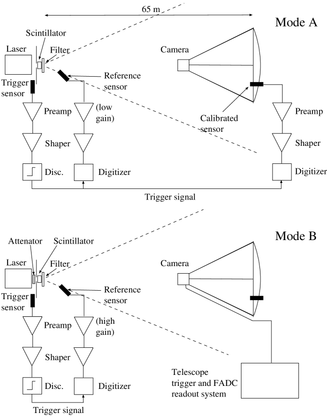
Fig. 1: Configurations used in mode A to calibrate the light intensity at the telescope, in in mode B to measure the telescope response.

3 Telecope calibration and systematic errors

Calibration measurements were taken at two center wavelengths, 430 nm and 470 nm, during two measurement campaigns. Based on the experience in the first campain, a number of sources of systematic errors were identified and corrected. We therefore use only the data from the second campaign. Poor weather conditions allowed only three sets of calibration measurements, at 430 nm and at 470 nm in one night, and a second 430 nm measurement in another night. In between, the setup was partly disassembled, so the comparison of the two measurements at 430 nm serves to test the reproduceability of the procedure. One measurement typically included 1000 or more laser shots; statistical errors are therefore generally small, and the precision of the calibration is entirely dominated by systematic effects. Figs. 2 through 4 show characteristic data from various steps of the procedure: the signal of the calibrated sensor at the telescope in calibration mode A (Fig. 2), the typical image detected in the camera in mode B (Fig. 3), and the intensity detected in the camera (Fig. 4) after processing with the usual analysis chain.

Fig. 2: Example for the distribution of pulse heights measured with the calibrated sensor at the telescope in mode A.

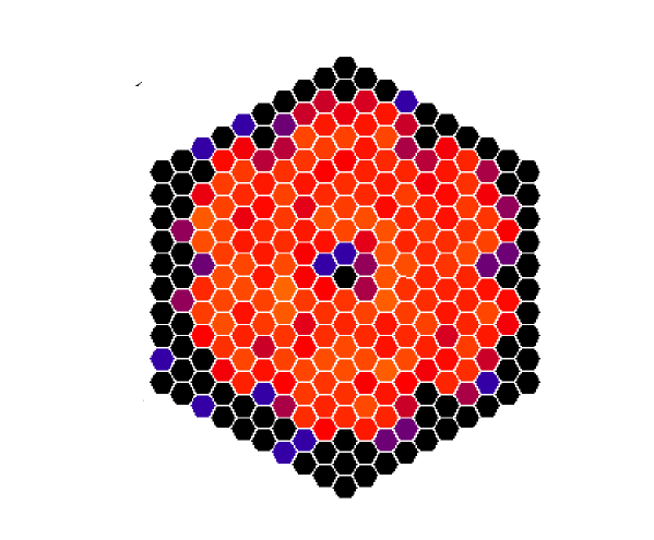
Fig. 3: A typical calibration light pulse, as viewed by the telescope camera in mode B. The illuminated pixels trace the somewhat irregular outer contour of the tesselated mirror; the hole in the center is caused by the shadow of the camera.

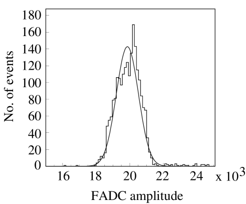
Fig. 4: Distribution of the total signals seen by the camera (in ADC units), for a typical calibration run.

The telescope sensitivity $K_{IACT}(\nu)$ is derived in the following steps:

• Using the photo diode calibration provided by the manufacturer, and the calibrated sensitivity of the charge amplification chain, the light flux in mode A is calculated from the averaged signal.

• Using the signals of the reference diode near the light source in modes A and B, and the calibrated gains of the low-gain and high-gain amplification chains, the attenuation factor between mode A and B and hence the flux at the telescope in mode B is calculated.

• Dividing the average IACT signal in mode B (in units of ADC counts) by the flux, the sensitivity $K_{IACT}$ is derived.

With this procedure, the parameters listed in Table 1 were derived. The two measurements at 430 nm, taken in different nights with a partial disassembly of the components in between, yield results which agree within 1.4%.

Wavelength [nm]	430 (I)	430 (II)	470
Photons/pulse, Mode A [1/cm2]	$9.90\cdot 10^{3}$	$9.48\cdot 10^{3}$	$2.99\cdot 10^{3}$
Attenuation	$6.01\cdot 10^{3}$	$6.01\cdot 10^{3}$	$1.92\cdot 10^{3}$
Photons/pulse, Mode B [1/cm2]	1.65	1.58	1.56
Total camera signal [ADC counts]	$1.99\cdot 10^{4}$	$1.88\cdot 10^{4}$	$1.39\cdot 10^{4}$
$K_{IACT}$ [ADC counts/(photon/cm2)]	$(1.21\pm 0.12)\cdot 10^{4}$	$(1.19\pm 0.12)\cdot 10^{4}$	$(0.89\pm 0.09)\cdot 10^{4}$
$K_{o}$ [ADC counts/(photon/cm2)]	$(1.13\pm 0.25)\cdot 10^{4}$	$(1.13\pm 0.25)\cdot 10^{4}$	$(0.81\pm 0.18)\cdot 10^{4}$

Table 1: Summary of the results of the calibration measurements, listing the mean number of photons per pulse in modes A and B, the attenuation between A and B, the average camera signals, the IACT sensitivity $K_{IACT}$ derived from these measurements, and the expected sensitivity $K_{o}$ based on a priori knowledge of telescope properties, and the measurement of the number of ADC channels per photoelectron (see section 4).

Apart from the practically negligible statistical errors, the following elements were considered as the major sources of systematic errors in the determination of $K_{IACT}$:

• the sensitivity and effective area of the calibrated photo diode at the telescope

• differences in the conditions during diode calibration and during actual use

• the absolute calibration of the amplification chain for the telescope diode

• the absolute calibration of the two (high-gain and low-gain) amplication chains used for the reference diode to determine the attenuation between modes A and B

• deviations from linearity of the camera pixels for large pulse heights

• a slight asymmetry in the distribution of IACT signals (Fig. 4)

• the uniformity of the illumination of the mirror, and the slight changes in light paths due to the relative proximity of the light source.

The calibrated photo diode (Hamamatsu S 3590-06) was specified with a sensitivity of 0.222 A/W at 430 nm, and 0.286 A/W at 470 nm, with errors of $\pm 5\%$. The effective area of the diode was determined by measuring the photocurrent for uniform illumination through a series of diaphragms with different diameters, and entirely without diaphragm. From the current with the fully illuminated diode, and the measured curve of current vs. illuminated area, the effective area $A$ of the diode was determined to $0.89\pm 2$ mm². The relevant product of sensitivity times effective area was checked against three other photo diodes (two Newport 818-UV/CM with $A=1.00$ cm², calibrated to $\pm$ 2% in the relevant wavelength region, and a Gigahertz SSO-BL-50-2-BNC with $A=0.50$ cm², calibrated to $\pm$ 4%) by uniformly illuminating the diodes; the results were in good agreement within the quoted errors.

The photo sensor used to measure the photon flux at the telescope is factory-calibrated at $25^{\circ}$C under continuous illumination without external bias. For our measurements, it was operated with short (ns) light pulses, and with a bias voltage of 28 V in order to deplete the diode and to minimize detector capacitance and hence noise. Temperatures were around $3^{\circ}$C to $5^{\circ}$C. Laboratory measurements showed that the application of the bias voltage increased the diode output by 1%. According to specifications, the diode calibration should apply both to DC mode (with a sensitivity expressed in A/W) and to pulsed mode (sensitivity in C/J). We verified that the sensitivity does not depend on the duty cyle of the light source, within 2% errors. Temperature dependence is more critical; while no specifications were given for the diode used in the setup, similar diodes show an increase of up to 4-5% in output at 430 nm, when the temperature is lower by $25^{\circ}$C compared to the calibration, and a reduced effect at 470 nm. Laboratory measurements showed indeed such a behaviour, within 2% to 3% errors. Corresponding correction factors were applied.

Two different techniques were used to calibrate the charge amplifiers. One method was to inject a defined amount of charge via a calibration capacitor. A problem with this technique is that for small capacitance values the measurement of the capacitance is non-trivial; for large capacitors errors may be introduced since the input impedance of the amplifier can no longer be neglected. We used capacitors between 2 and 20 pF, measured to 5% for $C<10$ pF and to 3% for larger values. Calibration results with the different capacitors were consistent. A second calibration technique was to use the actual photo detector to detected $\alpha$-radiation from ²⁴¹Am decays, thereby depositing a well-defined amount of charge in the actual detection device, without requiring any additional external elements. Source and detector were placed in a vacuum vessel to avoid energy loss in air. Fig. 5 shows a typical spectrum with two ²⁴¹Am lines of 5.443 MeV and 5.486 MeV. The resulting amplifier gains are listed in Table 2, together with the values obtained with the charge injection via capacitor. For the two high-gain amplifiers, both techniques give consistent results. For the low-gain amplifier, the methods deviate by 6.5%, or 1.5 standard deviations. No convincing explanation was found for this discrepancy. For the calculation of telescope sensitivity, we use the calibration constant obtained with the ²⁴¹Am source, but we enlarge the error to include the value obtained with the capacitor calibration.

Fig. 5: Pulse height distribution deteced when irradiating the calibrated photo diode with $\alpha$ particles from an Am source, with energies of 5.443 MeV and 5.486 MeV.

Gains in V/C	Capacitor charge injection	241Am source
High-gain amp., reference diode	$(1.69\pm 0.05)\cdot 10^{13}$	$(1.71\pm 0.03)\cdot 10^{13}$
Low-gain amp., reference diode	$(1.03\pm 0.03)\cdot 10^{10}$	$(0.96\pm 0.03)\cdot 10^{10}$
High-gain amp., telescope diode	$(1.52\pm 0.05)\cdot 10^{13}$	$(1.54\pm 0.03)\cdot 10^{13}$

Table 2: Gains of the diode readout chains (preamplifier and shping amplifier), measured with two different calibration techniques. The gains quoted refer to a low gain setting (‘20’) of the shaper amplifier; in most of the actual measurements, a higher (calibrated) gain (‘1000’) was used.

The calibration procedure at 430 nm resulted in pulse heights of some camera pixels of 180 and more photoelectrons. From earlier studies of the linearity of the PM and the amplification chain we know that at this pulse height deviations from linearity cannot be neglected, caused mainly by nonlinearities in the PM response. On average, pulse heights of those high pixels are 3% to 4% lower than expected for a linear response. A corresponding correction factor was applied, with an overall systematic error of 2%.

We note further that the distribution of the integral pulse height detected in the camera is not exactly symmetric (Fig. 4). Since the laser pulse height was monitored continously during the measurement, a drift of the laser signal can be excluded. A possible origin are imperfections in the digital signal processing; the amplitude derived from the flash-ADC signals depends slightly on the phase between the signal and the sampling clock. In principle, this effect is corrected, but residual effects at the percent level are possible. Since the same effect will occur for genuine Cherenkov signals, this small asymmetry should not influence the quality of the calibration, which refers to the average pulse height in both cases. We nevertheless assign a systematic error of 3% corresponding to the difference between the mean and the peak of the distribution.

Finally, there may be minor differences between the illumination of the mirror with the light source at a distance of about 60 m, and with Cherenkov light from ‘infinity’. To ensure that the mirror is uniformly illuminated, we rotated the light source by $\pm 10^{\circ}$, equivalent to a displacement of the axis of the source from the telescope by three times the mirror diameter; the amount of light detected at the telescope was constant within 2-3%. Differences in mirror obscuration between the slightly divergent beam from the source, and ideal parallel light are below 1%.

The resulting statistical and systematical errors are summarized in Table 3. To arrive at the final error given in Table 1, the various systematic errors were added in quadrature. The resulting total error is about 10%. Given the availability of photo sensors with 2% calibration errors, improved calibration procedures for the electronics, and better temperature control, we believe that with the further development of this technique an overall 5% error should be possible.

Error source	Error [%]
Statistical errors	$<0.4$
Calibration of telescope photo sensor	5.5
Difference between calibration and operation cond.	3.0
Electronics gain, telescope photo sensor	2.0
Electronics gain, reference sensor, low gain (mode A)	6.5
Electronics gain, reference sensor, high gain (mode B)	2.0
Nonlinearity of camera PMs	2.0
Asymmetry of distribution of camera signals	3.0
Uniformity of mirror illumination and geometry	1.5
Total error	10.2

Table 3: Sources of error in the determination of $K_{IACT}$. The PM nonlinearity is only relevant for the measurement at 430 nm, with its larger typical pulse heights. For the total error, the different systematic errors were added in quadrature.

4 Comparison with other calibration techniques

It is of course interesting the see how the sensitivities $K_{IACT}$ measured with the light source compare with other calibration techniques.

We consider primarily the approach where the individual factors contributing to $K_{IACT}$ are estimated individually, as listed in Table 4. The mirror area quoted includes the shadowing by the camera masts etc. The mirror reflectivity is assumed to $(85\pm 5)\%$ (compared to 89% measured for new mirrors [13]). Light collection by the camera PMs is governed by a thin plexiglas window (Röhm und Haas type 218, with improved transparency at short wavelengths), and by the funnels in front of the PMs. Data-sheet values are used for the PMT quantum efficiency, with a 15% uncertainty on these values. Losses in photoelectron collection between the cathode and the first dynode are neglected; since the funnels illuminate only the central 15 mm of the PMTs, with their nominal cathode diameter of 19 mm, such losses should be small. The response of the readout to a single photoelectron is determined based on the width of the laser test pulses used to flat-field the camera, after corrections for the width of the single-photoelectron response etc. Multiplying all these factors, one obtains the sensitivities $K_{o}$ given in Tables 4 and 1, which are in good agreement with the results from the optical calibration.

Mirror area	$8.0\pm 0.3$ m2
Mirror reflectivity	$85\pm 5$%
Plexiglas camera cover	$92\pm 1$%
Funnel light collectors	$91\pm 3$%
Quantum efficiency	$21\pm 3$% at 430 nm
	$15\pm 2$% at 470 nm
Conversion factor	$0.95\pm 0.14$ ADC counts/photoel.
$K_{o}$	$(1.13\pm 0.25)\cdot 10^{4}$ ADC counts/(ph./cm2) at 430 nm
	$(0.81\pm 0.18)\cdot 10^{4}$ ADC counts/(ph./cm2) at 470 nm

Table 4: Factors contributing to the estimate of $K_{o}$.

A second approach uses the measured cosmic-ray trigger rate of a telescope to derive its effective threshold and hence its effective sensitivity. While final numbers are still lacking, initial studies [14] indicate agreement within the typical errors of about 15%.

References

- [1] T.C. Weekes, Space Science Rev. 75 (1996) 1; M. F. Cawley and T.C.Weekes, Experimental Astronomy 6 (1996) 7.
- [2] A.M. Hillas, Space Science Rev. 75 (1996) 17.
- [3] F. Aharonian et al., Experimental Astronomy 2 (1993) 331.
- [4] C.W. Akerlof et al., Astrophys. J. 377 (1991) L97.
- [5] A. Daum et al., preprint astro-ph/9704098 (1997), Astroparticle Phys., in press; F. Aharonian et al., preprint astro-ph 970619 (1997).
- [6] R. Mirzoyan, Proceedings of the Int. Workshop “Towards a Major Atmospheric Cherenkov Detector IV”, Padua, (1995), M. Cresti (Ed.), p. 230.
- [7] T. Devlin et al., Nucl. Instr. meth. A268 (1988)24; W. Koska et al., FERMILAB-Pub-97/092 (1997).
- [8] A.G. Wright, J. Phys. E 14 (1981) 851.
- [9] A. Konopelko et al., Astroparticle Phys. 4 (1996) 199.
- [10] A. Plyasheshnikov et al., submitted for publication.
- [11] G. Vacanti et al., Astroparticle Phys. 2 (1994) 1.
- [12] O. Karschnick, Diploma Theses, Kiel (1996).
- [13] R. Mirzoyan et al., Nucl. Instr. Meth. A351 (1994) 513.
- [14] F. Aharonian, M. Hemberger, A. Konopelko, internal note (1996), unpublished.