Structure Detection in Low Intensity X-Ray Images

Abstract

In the context of assessing and characterizing structures in X-ray images, we compare different approaches. Most often the intensity level is very low and necessitates a special treatment of Poisson statistics. The method based on wavelet function histogram is shown to be the most reliable one. We also present a multi-resolution filtering method based on the wavelet coefficients detection. Comparative results are presented by means of a simulated cluster of galaxies.

1 Introduction

The ability of detecting structures in X-ray image of celestial objects is crucial, but the task is highly complicated due to the low photon flux, typically from $0.1$ to a few photons per pixel. Point sources detection can be done by fitting the Point Spread Function, but this method does not allow extended sources detection. One way of detecting extended features in a image is to convolve it by a Gaussian. This increases the signal to noise ratio, but at the same time, the resolution is degraded. The VTP method (Scharf et al. 1997) allows detection of extended objects, but it is not adapted for the detection of substructures. Furthermore, in some cases, an extended object can be detected as a set of point sources (Scharf et al. 1997). The wavelet transform (WT) has been introduced (Slezak et al. 1990) and presents considerable advantages compared to traditional methods. The key point is that the wavelet transform is able to discriminate structures as a function of scale, and thus is well suited to detect small scale structures embedded within larger scale features. Hence, WT has been used for clusters and subclusters analysis (Slezak et al. 1994; Grebenev et al. 1995; Rosati et al. 1995; Biviano et al. 1996), and has also allowed the discovery of a long, linear filamentary feature extended over approximatily 1 Mpc from the Coma cluster toward NGC 4911 (Vikhlinin et al. 1996). In the first analyses of images by the wavelet transform, the Mexican hat was used. The method simply consists in applying the correlation product between the image $I$ and the wavelet function:

$$w_{a}(x,y)=I(x,y)\otimes\psi(\frac{x}{a},\frac{y}{a})$$ (1)

Where $a$ is the scale parameter. By varying $a$, we obtain a set of images, each one corresponding to the wavelet coefficients of the data at a given scale. The wavelet function corresponding to the Mexican hat is

$$\psi(\frac{x}{a},\frac{y}{a})=(1-\frac{x^{2}+y^{2}}{a^{2}})e^{-\frac{(x^{2}+y^{2})}{2a^{2}}}$$ (2)

More recently the à trous wavelet transform algorithm has been used because it allows an easy reconstruction (Slezak et al. 1994; Vikhlinin et al. 1996). By this algorithm, an image $I(x,y)$ can be decomposed into a set $(w_{1},...,w_{n},c_{n})$,

$$I(x,y)=c_{n}(x,y)+\sum_{j=1}^{n}w_{j}(x,y)$$ (3)

Several statistical models have been used in order to say if a X-ray wavelet coefficient $w_{j}(x,y)$ is significant, i.e. not due to the noise. In Viklinin et al. (1996), the detection level at a given scale is obtained by an hypothesis that the local noise follows a Gaussian noise. In Slezak et al. (1994), the Anscombe transform was used in order to transform an image with a Poisson noise into an image with a Gaussian noise. Other approaches have also been proposed using k sigma clipping on the wavelet scales (Bijaoui & Giudicelli 1991), simulations (Slezak et al. 1990; Escalera & Mazure 1992, Grebenev et al. 1995), a background estimation (Damiani et al. 1996; Freeman et al. 1996), or the histogram of the wavelet function (Slezak et al. 1993; Bury 1995).

We discuss and compare in this paper the different methods for signal detection using the à trous wavelet transform algorithm and present how X-ray images can be restored even in the case of very low photon flux.

2 Detection Level Estimation in the Wavelet Space

2.1 Model and Simulation

Simulations can be used for deriving the probability that a wavelet coefficient is not due to the noise (Escalera et al. 1992). Modeling a sky image (i.e. uniform distribution and Poisson noise) allows determination of the wavelet coefficient distribution and derivation of a detection threshold. For substructure detection in a cluster, the large structure of the cluster must be first modeled, otherwise noise photons related by the large scale structure will introduce false detections at lower scales. If we have a physical model, Monte Carlo simulations can also be used (Escalera & Mazure, 1992; Grebenev et al. 1995), but this approach requires a long computation time, and the detections will always be model-dependent. Damiani et al. (1996), and also Freeman et al. (1996) propose to calculate the background from the data in order to derive the fluctuations due to the noise in the wavelet scales. It is regretable to have to do this, because we lose one the main advantage of the use of the wavelet transform, which is to be background-free. Indeed, wavelet coefficients have a null mean, and the detection is just done by comparison to a given threshold. Furthermore, background estimation is not an easy task, and generally requires several steps (filtering, interpolation, etc), and error estimation on the background is generally difficult to calculate.

2.2 Sigma Clipping

A straightforward method, initially proposed by (Bijaoui & Giudicelli 1991), for deriving the detection levels at each scale is to apply a sigma clipping at each scale. Therefore a standard deviation $\sigma_{j}$ is estimated at each scale $j$, and wavelet coefficients $w_{j}(x,y)$ are considered as significant if

$$\mid w_{j}(x,y)\mid>k\sigma_{j}$$ (4)

where $k$ is generally taken equal to 3. This method allows us to easily detect strong features, but is certainly not optimal for detection of weak objects. Indeed, as the noise is not Gaussian, it is difficult to estimate the real probability of false detection using this $k\sigma$ detection criterion.

2.3 Local Gaussian noise

Vikhlinin et al. (1995) proposed to assume a Gaussian local noise, and to estimate the map $I_{\sigma}(x,y)$ from the the local background. The standard deviation $\sigma_{j}(x,y)$ related to a wavelet coefficient $w_{j}(x,y)$ is derived from $I_{\sigma}(x,y)$ using the property of linearity of the wavelet transform (Starck & Bijaoui, 1994). As previously, the hypothesis is not true, and the consequence is the same. A solution is to use Monte Carlo simulations to set the correspondence between the standard deviation of a wavelet coefficient and the levels of significance (Grebenev et al, 1995), but the simulations must be performed for each image because the significance levels vary strongly with the number of photons (Grebenev et al, 1995).

2.4 Anscombe transform

In Slezak et al. (1994) and Biviano et al. (1996), the Anscombe transform

$$t(I(x,y))=2\sqrt{I(x,y)+\frac{2}{3}}$$ (5)

has been used and acts as if the data arose from a Gaussian noise with white model, with $\sigma=1$, under the assumption that the mean value of $I$ is large. Simulations have shown (Murtagh et al. 1995) that a number of photons less than 30 per pixel introduces a bias. In X ray images, the number of photons is often lower, and sometimes can even be equal to zero. Using Anscombe transform in this case will introduce an over estimation of the noise level. To overcome this difficulty, the noise standard deviation can be reestimated, for instance as in (Slezak et al 1994) i.e. by applying a sigma clipping at the first scale of the wavelet transform. However, this approach assumes that the noise is homogeneous, which is not true. Indeed, if the number of photons per pixel is lower that 30, the standard deviation of noise after Anscombe transformation, is varying strongly with the number of photons (Murtagh et al, 1995).

2.5 Wavelet Function Histogram

An approach for very small numbers of counts, including frequent zero cases, has been described in Slezak et al. (1993) and Bury (1994), for large scale clustering of galaxies. We have adopted here the same approach to analyze X-ray images.

A wavelet coefficient at a given position and at a given scale $j$ is

$$w_{j}(x,y)=\sum_{k\in K}n_{k}\psi(\frac{x_{k}-x}{2^{j}},\frac{y_{k}-y}{2^{j}})$$ (6)

where $K$ is the support of the wavelet function $\psi$ (i.e. the box in which $\psi$ is not equal to 0) and $n_{k}$ is the number of events which contribute to the calculation of $w_{j}(x,y)$ (i.e. the number of photons included in the support of the dilated wavelet centered at ($x$,$y$)).

If a wavelet coefficient $w_{j}(x,y)$ is due to the noise, it can be considered as a realization of the sum $\sum_{k\in K}n_{k}$ of independent random variables with the same distribution as that of the wavelet function ($n_{k}$ being the number of photons or events used for the calculation of $w_{j}(x,y)$). Then we compare the wavelet coefficient of the data to the values which can taken by the sum of $n$ independent variables.

The distribution of one event in the wavelet space is directly given by the histogram $H_{1}$ of the wavelet $\psi$. Since independent events are considered, the distribution of the random variable $W_{n}$ (to be associated with a wavelet coefficient) related to $n$ events is given by $n$ autoconvolutions of $H_{1}$

$$H_{n}=H_{1}\otimes H_{1}\otimes...\otimes H_{1}$$ (7)

Fig. 1 shows the shape of a set of $H_{n}$. For a large number of events, $H_{n}$ converges to a Gaussian.

Figure 1: Autoconvolution histograms for the wavelet associated with a B₃ spline scaling function for 1 and 2 events (top left), 4 to 64 events (top right), 128 to 2048 (bottom left), and 4096 (bottom right).

In order to facilitate the comparisons, the variable $W_{n}$ of distribution $H_{n}$ is reduced by

$$c=\frac{W_{n}-E(W_{n})}{\sigma(W_{n})}$$ (8)

$E$ being the mathematical expectation, and the cumulative distribution function is

$$F_{n}(c)=\int_{-\infty}^{c}H_{n}(u)du$$ (9)

From $F_{n}$, we derive $c_{min}$ and $c_{max}$ such that $F(c_{min})=\epsilon$ and $F(c_{max})=1-\epsilon$.

Let us define a reduced wavelet coefficient as

$$w^{r}_{j}(x,y) = \frac{w_{j}(x,y)}{\sqrt{n}\sigma_{\psi_{j}}}$$ (10)

$$= \frac{w_{j}(x,y)}{\sqrt{n}\sigma_{\psi}}4^{j}$$ (11)

where $\sigma_{\psi}$ is the standard deviation of the wavelet function, $\sigma_{\psi_{j}}$ is the standard deviation of the dilated wavelet function ($\sigma_{\psi_{j}}=\sigma_{\psi}/4^{j}$), and $w_{j}(x,y)$ a wavelet coefficient obtained using the à trous wavelet transform algorithm.

Therefore a reduced wavelet coefficient, $w^{r}_{j}(x,y)$, calculated from $w_{j}(x,y)$, and resulting from $n$ photons or counts is significant if:

$$F(w^{r})>c_{max}$$ (12)

or

$$F(w^{r})<c_{min}$$ (13)

This detection method presents several advantages: it is independent of any model, no simulation is needed, and it is theoretically rigorous.

3 Image Filtering

We propose here to filter an image using the multiresolution support, which is determined from the significant wavelet coefficients (i.e. coefficient which are not due to the noise).

3.1 Multiresolution Support

A multiresolution support of an image describes in a logical or Boolean way if an image $I$ contains information at a given scale $j$ and at a given position $(x,y)$. If $M^{(I)}(j,x,y)=1$ (or $=\ true$), then $I$ contains information at scale $j$ and at the position $(x,y)$. $M$ depends on several parameters:

• The input image.

• The algorithm used for the multiresolution decomposition.

• The noise.

• All additional constraints we want the support to satisfy.

Such a support results from the data, the treatment (noise estimation, etc.), and from knowledge on our part of the objects contained in the data (size of objects, linearity, etc.). In the most general case, a priori information is not available to us.

The multiresolution support of an image is computed in several steps:

• Step one is to compute the wavelet transform of the image.

• Binarization of each scale leads to the multiresolution support (the binarization of an image consists in assigning to each pixel a value only equal to $0$ or $1$).

• A priori knowledge can be introduced by modifying the support.

This last step depends on the knowledge we have of our images. For instance, if we know there is no interesting object smaller or larger than a given size in our image, we can suppress, in the support, anything which is due to that kind of object. This can often be done conveniently by the use of mathematical morphology. In the most general setting, we naturally have no information to add to the multiresolution support.

The multiresolution support will be obtained by detecting at each scale the significant coefficients. The multiresolution support is defined by:

$$M(j,x,y)=\left\{\begin{array}[]{ll}\mbox{ 1 }&\mbox{ if }w_{j}(x,y)\mbox{ is significant}\\ \mbox{ 0 }&\mbox{ if }w_{j}(x,y)\mbox{ is not significant}\end{array}\right.$$ (16)

3.2 Hard thresholding

In the previous section, we have shown how to detect significant structures in the wavelet scales. A simple filtering can be achieved by thresholding the non-significant wavelet coefficients, and by reconstructing the filtered image by the inverse wavelet transform. In the case of the à trous wavelet transform algorithm, the reconstruction is obtained by a simple addition of the wavelet scales and the last smoothed array. The solution $S$ is

$$S(x,y)=c_{p}^{(I)}(x,y)+\sum_{j=1}^{p}M(j,x,y)w_{j}^{(I)}(x,y)$$ (17)

where $w_{j}^{(I)}$ are the wavelet coefficient of the input data, and $M$ is the multiresolution support.

3.3 Iterative thresholding

As the à trous wavelet transform algorithm is a non orthogonal wavelet transform algorithm, the wavelet transform of the solution $S$ does not produce wavelet coefficients $w_{j}^{(S)}(x,y)$ which are exactly equal to $M(j,x,y)w_{j}^{(I)}(x,y)$. This is evidently not a problem for wavelet coefficients where nothing was detected ( $M(j,x,y)=0$), but it means that an error has been introduced during the reconstruction of objects from the significant structures. This can be corrected using an iterative method (Starck et al., 1995). If a wavelet coefficient of the original image is significant, then the multiresolution coefficient of the residual image (i.e. $w^{(R^{(n)})}_{j}$ with $R=I-S$) must be equal to zero. This is obtained by the following iteration:

$$S^{k+1}(x,y) = S^{k}(x,y)+c_{p}^{(R)}(x,y)$$ (19)

$$+\sum_{j=1}^{p}M(j,x,y)w_{j}^{(R)}(x,y)$$

Thus the regions of the image which contain significant structures at all levels are not modified by the filtering. The residual will contain the value zero over all of these regions. If an object is close to another one, which has the same size and has a stronger flux, it is possible that we will not detect it because of the negative component around the detected structure of the second object (this is due to fact that a wavelet function has null mean). But after one or two iterations, the solution will contain the second object, and the residual will contain only the first one. This means that the wavelet coefficient (obtained from the residual) of the first object will no longer be masked by the second. The multiresolution support can be updated by reducing the wavelet coefficient of the residual image (see 11), and applying both comparison tests of eqn 12 and eqn 13. Note that $c_{min}$ and $c_{max}$ are not recomputed, because the detection level is unchanged.

The algorithm becomes:

1. $k\leftarrow 0$.

2. Initialize the solution, $I^{(0)}$, to zero.

3. Determine the multiresolution support of the image.

4. Determine the residual, $R^{(k)}=I-S^{(k)}$.

5. Update the multiresolution support of the image.

6. Determine the wavelet transform $w^{(R)}$ of $R^{(k)}$.

7. Threshold: only retain the coefficients which belong to the support.

8. Reconstruct the thresholded residual image. This yields the image $\tilde{S}^{(k)}$ containing the significant residuals of the residual image.

9. Add this thresholding residual to the solution: $S^{(k)}\leftarrow S^{(k)}+\tilde{S}^{(k)}$.

10. If $\mid(\sigma_{R^{(k-1)}}-\sigma_{R^{(k)}})/\sigma_{R^{(k)}}\mid\ >\ \epsilon$ then $k\leftarrow k+1$ and goto 4.

A positivity constraint can be introduced in the algorithm by thresholding at each iteration negative values in the solution $S$. The multiresolution can also be updated, following each iteration, using the wavelet coefficients of the residual image:

$$M^{(n+1)}(j,x,y)=\left\{\begin{array}[]{ll}1&\mbox{if }w^{(R)}_{j}(x,y)\mbox{ is significant }\\ &\mbox{ or }\ M^{(n)}(j,x,y)=1\\ 0&\mbox{if }w^{(R)}_{j}(x,y)\mbox{ is not significant }\\ &\mbox{ and }\ M^{(n)}(j,x,y)=0\end{array}\right.$$ (24)

This is of interest when an object is hidden by another one. It appends each time a faint object is close to a stronger one. Then the faint object is undetectable due to the negative coefficients which surrounded the strong one. But after one or two iterations, the strong object does not affect the residual, and the faint object may be appear in the scales.

3.4 Filtering as an inverse problem

The filtering can be seen as an inversed problem. Indeed, we want to reconstruct an image from the detected wavelet coefficient. The problem of reconstruction (Bijaoui and Rué 1995) consists in searching a signal $S$ such that its wavelet coefficients are the same as those of the detected structure. By noting $\cal T$, the wavelet transform operator, and $P$ the projection operator in the subspace of the detected coefficients (i.e. set to zero all coefficients at scales and positions where nothing where detected), the solution is found by minimization of

$$J(S)=\parallel W-(P\circ\cal T)S\parallel$$ (25)

where $W$ represents the detected wavelet coefficients of the image $I$. A complete description of algorithms for minimization of such an equation can be found in Bijaoui and Rué (1995). In practice, compared to the previous algorithm, the main modification is the introduction of the adjoint wavelet transform operator, replacing the step 8 (reconstruction).

3.5 Conclusion

A simple thresholding generally provides poor results. Artifacts appear around the structures, and the flux is not preserved. The multiresolution support filtering requires only a few iterations, and preserves the flux. The use of the adjoint wavelet transform operator instead of the simple coaddition of the wavelet scale for the reconstruction (step 8 of the algorithm) suppresses the artifacts which may appear around objects. In fact, the algorithm is analogous to minimizing the equation 25. The use of the Van Cittert algorithm for minimization of $J$ leads to the modified multiresolution support filtering method. Other approaches for the minimization can also be used (conjugate gradient, etc). The Van Cittert algorithm is not optimal for the time computation, but it has the advantage of allowing us to add constraints during the iterations. The positivity is a strong constraint which should be used. Other additional prior knowledge can be added. For instance, such prior knowledge could be in the form of a star position catalog, bad pixel positions, a given position where we expect the object to be located, or constraints on the size of the object. Hence the multiresolution constraint allows us to integrate into the same data structure other information sources (catalogs, images, etc.) and prior knowledge (positions, object sizes, etc.), in a way which facilitates subsequent image processing operations. In the most general case, we do not have such prior information available, so the multiresolution support is computed from the given input image and its noise properties.

Partial restoration can also be considered. Indeed, we may want to restore an image which is background free, objects which appears between two given scales, or one object in particular. Then, the restoration must be performed without the last smoothed array for a background free restoration, and only from a subset of the wavelet coefficients for the restoration of a set of objects (Bijaoui et Rué 1995).

4 Noise Models Comparison

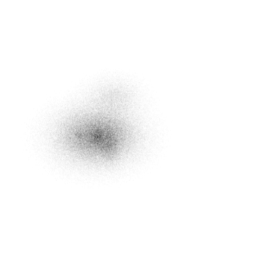
Figure 2: Left, simulated image. The central luminosity is equal to 12, and the two first isophots are at $1$ and $2.62$. Right, same image with a Poisson noise.

Fig. 2 (left) shows a simulated image of a galaxy cluster. Two point sources are superimposed (on the left of the cluster), a cooling flow is at the center, a substructure on its left, and a group of galaxies at the top. From this image, a “noisy” images has been created (Fig. 2 (right)). The mean background level is equal to 0.1 events per pixel. This corresponds typically to X-ray cluster observations. In the noisy image, the maximum value is equal to 23 events. The background is not very relevant. The problem in this kind of images is the small number of photons per object. It is very difficult to extract any information from them.

Figure 3: Top left and right, convolution of the noisy image with a Gaussian with a standard deviation equal to 3 and 5 respectively. Bottom left, filtered image using a sigma clipping on each wavelet scale, and a 10 sigma detection. Bottom right, filtered image using an hypothesis of local Gaussian noise, and a 10 sigma detection.

Fig. 3, top left and top right, shows the filtering of the image by convolving the noisy image by a Gaussian, with a standard deviation equal to 3 and 5 respectively. Using the Anscombe transform, we were unable to obtain an image with a reasonable quality. It seems that this transform should only be used in the condition defined in Murtagh et al (1995), i.e. with a minimum number of photons equal to 30 per pixel. In the case of very low photons count, the results are very poor.

Fig. 3 bottom left shows the result after a filtering using a sigma clipping on each wavelet scale, and a ten sigma detection. Fig. 3 bottom right shows the filtering using an hypothesis of local Gaussian noise, and a ten sigma detection. For both, even at a detection level of ten sigma, the filtered image presents residual noise.

Figure 4: Results of the filtering using the method based on the histogram autoconvolutions. Left, image obtained with a confidence level equal to $1e-3$ (which is equivalent to a $3.09$ sigma detection for the case of Gaussian noise), and right, image obtained with a confidence level equal to $10^{-4}$ ($3.72\sigma$ Gaussian equivalence).

Figure 4 shows the results of the filtering using the method based on the histogram autoconvolutions with two different confidence levels. Figure 4 left corresponds to a confidence interval of $10^{-3}$ (which is equivalent to a $3.09$ sigma detection for the case of Gaussian noise), and figure 4 right, with a confidence level equal to $10^{-4}$ ($3.72$ Gaussian equivalence). Even if the two point sources could not have been distinguished by eye in the noisy image, they have been detected and correctly restored.

Figure 5: Filtering of the simulated image with different background levels. From left to right and top to bottom, the background level was respectively equal to $0.1$, $0.5$, $1$, $2$ counts per pixel.

Figure 5 shows the result of the filtering with different background levels. The detections in the wavelet scale were done using $\epsilon=10^{-4}$. From left to right and top to bottom, the background level was respectively equal to $0.1$, $0.5$, $1$, $2$ counts per pixel. If the background level is high, there is more noise, and we see that the second source disappears when the background level increases, which is normal behavior.

The best filtering is clearly obtained using the method based on wavelet transform and the histogram autoconvolutions. For other methods which use the wavelet transform, we did not use Monte Carlo simulations and the exact level for signal detection is difficult to find. Furthermore, the level is certainly not the same for the whole scale. For this reason, a simple Gaussian filtering seems to be better.

5 Detected Structure Analysis

Once the significant wavelet coefficients have been detected, they can be grouped into structures (a structure is defined as a set of connected wavelet coefficients at a given scale), and each structure can be analyzed independently. Interesting information which can be easily extracted from an individual structure includes the first and second order moments, the angle, the perimeter, the surface, and the deviation of shape from sphericity (i.e. $4\pi\frac{Surface}{Perimeter^{2}}$). From a given scale, it is also interesting to count the number structures, and the mean deviation of shape from sphericity.

Figure 6: Left, multiresolution support of the simulated image (see figure  2). Right, multiresolution support of the same simulated field, but all objects contains less flux. The maximum of the noisy image is equal to 7.

In order to visualize the structures, we can create an image by plotting a contour for each detected structure. This provides a compact way to visualize the multiresolution support. Figure 6 (left) shows the contours of the multiresolution support of the simulated image of Section 4. Figure 6 (right) shows the contours of the same simulated field, but the objects of the simulated noisy image contain less flux (the maximum of the image is equal to seven counts), while the background is the at the same level ($0.1$ count per pixel). We can easily see that in this case, the two point sources have disappeared. Both detection were done with $\epsilon=10^{-4}$.

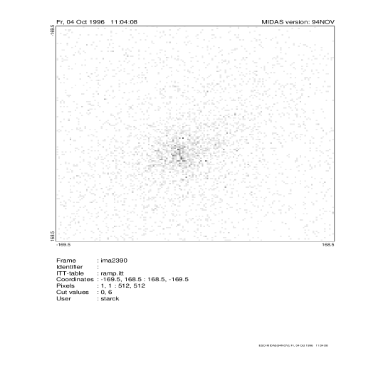
Figure 7: ROSAT image of the cluster A2390.

6 A2390 cluster filtering

The cluster of galaxies A2390 is located at a redshift of 0.231. Figure 7 shows an image of this cluster, obtained with ROSAT satellite. The resolution is one arc second per pixel, with a total number of 13506 photons for exposure time of approximately 8 hours. The background level is around 0.04 photons per pixel. It is clear that the raw data are not usable, and we need to filter it in order to extract the information. The standard method consists in convolving the image by a Gaussian. Figure 8 shows the result after applying this convolution (Gaussian with a full width at half maximum equal to 5”, which is approximatively the size of the instrumental response). The smoothed image shows structure, but we see also that a lot of noise remains, and it is difficult to assign a significance to these structures. Figure 9 shows the filtered image by the histogram based wavelet method. The noise has been eliminated, and we see that the wavelet transform has enhanced weak structures in the X-ray emission, which could explain the gravitational amplification phenomena which have been observed in the optical domain (Pierre et al. 1996).

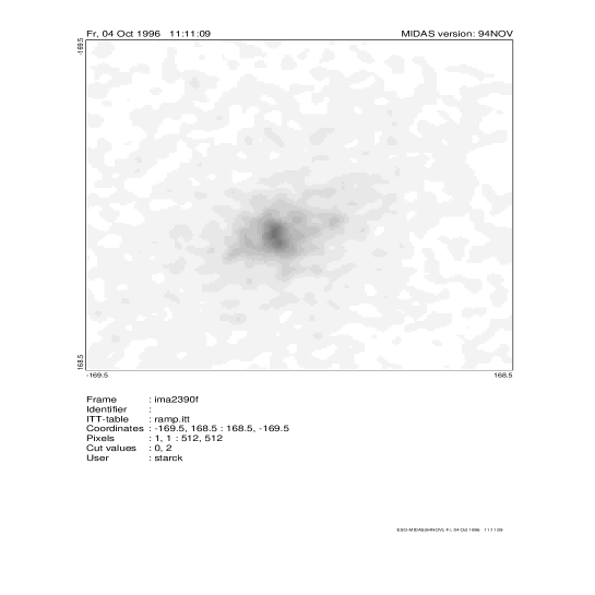
Figure 8: A2390 ROSAT image filtered by a standard method (convolution with a Gaussian).

Figure 9: A2390 ROSAT image filtered by the wavelet based method.

7 Conclusion

Simulations have shown that the best filtering approach for images containing Poisson noise with few events is the method based on the histogram autoconvolutions. This method allows one to give a probability that a wavelet coefficient is due to noise. No background model is needed, and simulations with different background levels have shown the reliability and the robustness of the method. Other noise models in the wavelet space lead to the problem of the significance of the wavelet coefficient. A ten sigma detection was not strong enough in our simulation to produce a good filtered image. In this case, only Monte Carlo simulations can allow one derivation of a good detection level, and then, a new problem appears of defining the correct background. The main advantage of the histograms based method is its independence of the background.

- [1] Anscombe, F.J., 1948, Biometrika 15, 246.
- [2] Bijaoui, A., Rué, F., 1995, ”A multiscale vision model adapted to the astronomical images”, Signal Processing, 46, 345–362.
- [3] Biviano, A., Durret, F., Gerbal, D., Le Fèvre, O., Lobo, C., Mazure, A., and Slezak, E., 1996, A&A311, 95–112.
- [4] Bury, P., 1995, Thesis, University of Nice-Sophia Antipolis.
- [5] Damiani, F., Maggio, A., Micela, G., Sciortino, S, 1996, in ADASS V, eds G.H. Jacoby and J. Barnes, ASP Conf. Ser., 101, 143.
- [6] Escalera, E., Slezak, E., and Mazure, A., 1992, A&A, 264, 379.
- [7] Escalera, E., Mazure, A., 1992, ApJ, 388, 23–32.
- [8] Freeman, P.E., Kashyap, V., Rosner, R., Nichol, R., Holden, B, Lamb, D.Q., 1996, in ADASS V, eds G.H. Jacoby and J. Barnes, ASP Conf. Ser., 101, 163.
- [9] Grebenev, S.A., Forman, W., Jones, C., and Murray, S., 1995, ApJ, 445, 607–623.
- [10] Murtagh, F., Starck, J.L., and Bijaoui, A., 1995, A&A, Suppl. Ser. 112, 179–189.
- [11] Pierre, M., Le Borgne, J.F., Soucail, G., and Kneib, J.P., 1996, A&A, 311, 413.
- [12] Rosati, P., Della Ceca, R., Burg, R., Norman, C., and Giacconi, R., 1995, Apj, 445, L11.
- [13] Scharf, C.A., Jones, L.R., Ebeling, H., Perlman, E., Malkan, M., and Wegner, G., 1997, ApJ, 477, 79–92.
- [14] Slezak, E., Bijaoui, A., Mars, G., 1990, A&A, 227, 301.
- [15] Slezak, E., de Lapparent, V. and Bijaoui, A. 1993, ApJ, 409, 517.
- [16] Slezak, E., Durret, F. and Gerbal, D., 1994, AJ, 108, 1996.
- [17] Starck, J.L., Bijaoui, A., 1994, Signal Processing, 35, 195–211.
- [18] Starck, J.L., Bijaoui, A., and Murtagh, F., 1995, in CVIP: Graphical Models and Image Processing, 57, 5, 420-431.
- [19] Vikhlinin, A., Forman, W., and Jones, C., 1996, astro-ph/9610151.