A Possible Dynamical Effect of a Primordial Magnetic Field

Abstract

The possible existence of a primordial magnetic field in the universe has been previously investigated in many articles. Studies involving the influence of a magnetic field in the nucleosyntesis era, studies considering the effects in the formation of structures during the radiation era and the matter era have been considered. We here assume the existence of a primordial magnetic field and study its effect, in particular, in the formation of voids. The study is twofold: to put constraints on the strength of the magnetic field during the recombination era and to preview its effects on the formation of voids.

1 Introduction

The existence of a primordial magnetic field is an old and still open problem in cosmology (see, e.g., Peebles (1993), for some discussion). For cosmological scales we may have $<\bf B>=0$, but there might well exist random magnetic fields at smaller scales (sub-horizon ones) such that $<B^{2}>\neq 0$.

Magnetic fields have been detected such as in high resolution Faraday rotation measurements made by Kronberg et al. (1990) of 3C191. The magnetic field strength in this z=1.945 system was found to be $\sim 0.4-4\mu G$.

Vallee (1990) using a sample of 309 galaxies and quasars obtained an upper limit of $10^{-9}G\times(0.01/\Omega_{IGM})$ (where $\Omega_{IGM}$ is the ratio between the ionized gas density in the IGM and the critical density, and h is the Hubble constant in units of 100 km s^-1 Mpc^-1) on the strength of the cosmological magnetic field which is coherent on horizon scales. This limit is reduced to $3\times 10^{-9}G\times(0.01/\Omega_{IGM})$ if the cosmic field is coherent only on scales of 10Mpc (see, e.g., Kronberg (1994)). Magnetic fields of $\sim 10^{-6}$ G is observed to be present in spiral galaxies (see, e.g., Kronberg (1994)), and also in Lyman-$\alpha$ clouds at high redshift, $z\sim 3$ (see, e.g., Peebles (1993)). It is not clear, however, how such fields were produced.

It is worth mentioning that studies of cluster Faraday rotations have been performed by some authors (see, e.g., Ge and Owen (1993)) in trying to look for primordial magnetic fields.

For galaxies, for example, there is no consensus concerning the origin of the magnetic field; some authors argue that dynamos could account for the growth of putative seed fields, but the magnetic field could well be primordial. The dynamo is a possible processes to amplify seed magnetic fields (see, e.g., Vainshtein and Ruzmaikin 1972a , b among others).

Some authors argued that a magnetic field could provide the primordial spectrum of density perturbations which would then be gravitationally amplified (see, e.g., Battaner et al. (1996)). In fact, if we consider that the magnetic field can be the source for the formation of the structures of the universe, we have the same problem that we have when we try to explain the production of density perturbations, i.e., the problem concerning the origin of such a seed magnetic field.

An important question concerning magnetogenesis has to do with its production epoch; some authors argue that it could occur in the inflationary era (see, e.g., Ratra (1992)). Ratra (1992) showed that fields produced from the inflationary era could have a strength of $B\sim 10^{-9}G$ at the present time.

Earlier papers by, for example, Harrison (1973) suggested that primordial turbulence during the radiation era could produce seed fields, that could be stocastically amplified, producing at the recombination era $B\sim 1G$. Quashnock et al. (1989) argued that magnetic fields could be created at the cosmological QCD phase transition. They obtained that fields corresponding to $B\sim 10^{-17}G$ by the time of the recombination era could be produced.

Zweibel (1988) considered a scenario in which density fluctuations, combined with tidal torques arising between mass condensations, causes regeneration of a seed field.

The detection of primordial magnetic fields, as argued by some authors (see Kosowsky and Loeb (1996)), is possible. Kosowsky and Loeb (1996) argued that primordial fields, that could be present at the last scattering surface, could induce a measurable Faraday rotation in the polarization of the cosmic background radiation. They argued that statistical detection of magnetic fields, that would correspond to present day magnetic fields as small as $10^{-10}$ G, would be possible.

Void regions in the distribution of galaxies are widely accepted as part of the structure of the universe. The observations show that void regions of diameter of up to $\sim 50h^{-1}$ Mpc are present in the universe. In a recent study by El-Ad et al. (1996), studying the new SSRS2 redshift survey (da Costa et al. (1994)), voids of diameter of $37\pm 8h^{-1}$ Mpc were found.

Concerning the formation of voids, three different mechanisms have been considered: 1) they may be formed during the formation of the structures of the universe, in particular, during the clustering processes; 2) through negative density perturbations; or 3) by explosions of pre-galactic objects or quasars.

It is worth mentioning that it is not completely clear how the big voids, that range from 10-100 Mpc, have been formed, due to the fact that the above three possibilities have problems to account for very big voids.

In the present work we study a possible dynamical effect that magnetic fields of a given strength and topology can produce in the formation of structures, in particular, in the formation of void regions. It is not our aim to study MHD in an expanding universe, some important studies have recently dealt with such an issue (see, e.g., Holcomb (1990))

We are not concerned here with the production of a primordial magnetic field. We consider that it could be produced primordially. We use strengths that are consistent with the constraints imposed by studies concerning the primordial nucleosynthesis and with the fields observed in the intergalactic medium and in galaxies.

Studies concerning the effect of a magnetic field on cosmological nucleosynthesis indicate that fields of 0.1 - 1 G at the recombination era are allowed (see, e.g., Cheng et al. (1994); Grasso nd Rubinstein (1996)). Considering that we would have at the present epoch fields of cosmological origin of $B\sim 10^{-8}-10^{-9}$ G, we would have at the recombination era $B\sim 0.001-0.1G$.

We study magnetic fields of strength $B=0.001-1G$ starting our calculations at the recombination era. We take into account a series of physical processes, described in detail in the next section, present during and after the recombination era, as well as the expansion of the universe. In the present study we consider a baryonic universe, therefore there is no dark matter (non-baryonic) in our model.

In section 2 we present the model studied, in which we include the basic equations. In section 3 we present and discuss our results, and finally in section 4 we present the main conclusions of our study.

2 Basic Equations

Our aim is to study the effects that primordial magnetic fields could cause in the formation of the structures of the universe. In particular, our concern in the present work is to study whether primordial magnetic fields of a given strength and topology could form void regions. On the other hand, our study imposes constraints on the possible strength of primordial magnetic fields.

The dynamical effects of magnetic fields depend strongly on their particular topology. In a given cloud the magnetic field can shrink or expand the cloud.

We choose here a topology that produces an outward pressure; in this way, the cloud, due to the magnetic thrust, expands.

When magnetic fields are present we use magneto-hydrodynamics to follow their effects. We consider ideal magneto-hydrodynamics where the conductivity is infinite, with the magnetic field frozen into the matter, in such a way that the magnetic flux is conserved and the changes of the magnetic field are given by:

$${\partial\vec{B}\over\partial t}=\nabla\times(\vec{v}\times\vec{B})$$

where $\vec{v}$ is the velocity field of the region where $\vec{B}$ is present.

We assume that the magnetic field is present in a finite region of space and within this region we define a coordinate system in such a way that the field is in the Z direction. The topology is chosen in such a way that the magnetic force acts in the R (radial cylindrical coordinate) direction, in particular, in the outward direction. Such a field can be written as:

$$\vec{B}=B_{rec}\biggl{(}{\bar{R}_{rec}\over\bar{R}_{\quad}}\biggr{)}^{2}\sqrt{1-\Big{(}{R\over\bar{R}}\Big{)}^{2}}\hat{Z}$$ (1)

where: $B_{rec}$ is the magnetic field along the Z axis at the recombination era, $\bar{R}_{rec}$ the radius of a spherical region that encompasses the field region at the recombination era, $\bar{R}$ the equatorial radius of the region, and R the radial cylindrical coordinate. Note also that this magnetic field goes to zero at the finite radius $\bar{R}$ as $\sqrt{1-(R/\bar{R})^{2}}$. Such a field has obviously an axial symmetry, but we are going to consider that it is present in a region that we consider to be initially spherical. This is in fact a rough approximation but it gives information on how such a field can influence that region. To follow in detail an actual situation in which a magnetic field is present, we need to consider a series of effects very difficult to deal with, even considering very complex models that involve the three spatial coordinates and time.

The magnetic field given by Eq. 1 satisfy the equation for flux conservation if $\vec{v}\propto\vec{R}$. A velocity field linear in $\vec{R}$ (and also in $\vec{Z}$) is consistent with a cloud contracting or expanding with uniform density. This very fact has been the main reason for the particular topology that we have chosen. As a result, as we will see below, the set of differential equations to be solved depends only on time.

Mestel (1965), for example, in his study on the problem of star formation in the presence of a magnetic field, also adopted the same topology that we have adopted here. He did so assuming the same argumentation that we have used, i.e., to maintain the density uniform where the field is present.

Still concerning Eq. 1, it represents a generic simple magnetic topology of the simplest current configuration of a magnetic fluctuation discussed in the literature - a current loop. A magnetic field configuration is associated with a current configuration from Maxwell’s equations. A current loop tends to expand. The opposite sides of the loop repel each other by the Biot-Savart law. Instead of treating the expansion of the current loop it is easier to treat the expansion of the magnetic field that it creates due to the magnetic pressure acting on the external medium. Thus the expansion due to the magnetic pressure of the magnetic topology of Eq. 1 describes the expansion of a simple current configuration such as the current loop which expands due to the Biot-Savart law. A simple current loop is very stable. The universe is highly conductive and current loops greater than $\sim 10^{13}cm$, by the time of the recombination era, did not dissipate on a Hubble time (see, e.g., Cheng et al. (1994)).

To follow the region in which the field is present we must solve the magneto-hydrodynamic equations, namely:

$${\partial\rho\over\partial t}+\nabla.\rho\vec{v}=0$$ (2)

the continuity equation;

$${d\vec{v}\over dt}+\nabla\phi+{1\over\rho}\nabla(P+P_{m})+{\sigma bT^{4}_{r}\over m_{p}c}x(\vec{v}-H\vec{r})=0$$ (3)

the equation of motion, where the last term is the photon-drag due to the cosmic background radiation;

$$\nabla^{2}\phi=4\pi G\rho$$ (4)

the Poisson equation for the gravitational potential;

$$P=N\rho kT(1+x)$$ (5)

the equation of state;

$$P_{m}={B^{2}\over 8\pi}$$ (6)

the magnetic pressure; and

$${du\over dt}=-L+{P\over\rho^{2}}{d\rho\over dt}$$ (7)

the energy equation.

In the above equations: $\rho$ is the matter density, $\vec{v}$ the velocity, $\phi$ the gravitational potential, $P$ the matter pressure, $P_{m}$ the magnetic pressure, $H\vec{r}$ the Hubble flow, $H=\dot{a}/a$ with $a$ and $\dot{a}$ being the scale factor and its time derivative, respectively, $T_{r}$ the background radiation temperature, $T$ the matter temperature, $x$ the degree of ionization, $u$ the energy density, $L$ the cooling function, $\sigma$ the Thomson cross section, $b=4/c$ times the Stefan Boltzmann constant, $m_{p}$ the proton mass, $c$ the velocity of light, $G$ the universal gravitational constant, $N$ the Avogrado’s number, and finally $k$ the Boltzmann constant.

For the degree of ionization we follow the article by Peebles (1968) in which the processes of recombination are taken into account in detail.

In the cooling function a series of processes have been taken into account: photon cooling (heating), recombination, Lyman-$\alpha$, and $H_{2}$ molecules. In the present work we obtained that the most relevant mechanism is photon cooling (heating).

It is worth stressing that it is not necessary to consider the putative losses via the presence of magnetic fields in the present study. It could be important in principle, but it is the photon-cooling (heating) that dominates the cooling-heating processes throughout the recombination era. These very processes maintain the matter temperature ($T_{m}$) close to the temperature of the background radiation ($T_{r}$) until the decoupling time. Yet, the thermal pressure is not important in the formation of the void region, the main mechanism that influences the formation of void region is the photon-drag (besides the magnetic thrust) that tries to inhibit any relative motion between the baryonic matter and the background radiation. The photon-drag depends on the radiation temperature to the fourth power and linearly on the degree of ionization. The degree of ionization depends on (during the recombination era) the photoionization rate (that depends on $T_{r}$) and on the recombination rate (that depends on $T_{m}$ ($\sim T_{r}$)).

After the decoupling time, other processes could be important, in particular in what concerns the thermal evolution of the void region. However, the size of such a void region does not depend on these other processes, since the thermal pressure is not important, and by this time neither the magnetic pressure is important.

To resolve the above set of equations we integrate it only in time. This is so due to the following reasons. First, the magnetic force, the photon-drag and the gravitational force depend on R and the Z coordinates linearly inside the region where the field is present. This implies that the velocity depends linearly on the above mentioned coordinates multiplied by a function of time. Second, due to the fact that the linear profile in the velocity is maintained throughout the region of interest the density profile is, as a consequence, uniform. The density in the region of interest as a consequence depends only on time. Similar models, but without taking into account the presence of magnetic fields, were developed by de Araujo and Opher (1989, 1990, 1991, 1993 and 1994) to study the formation of Population III objects, galaxies and voids. In fact, the difference between the present work and our latter studies is the inclusion of the magnetic term in the equation of motion.

From the above we see why the particular topology has been chosen. The aim is to have a magnetic pressure gradient producing an outward force that would maintain the density profile uniform in the region where the field is present. Any other topology produces a magnetic force that destroys the “top-hat” profile. To follow the evolution of the region where the field is present would then require the integration of the hydrodynamic equations not only on time but also on the R and Z coordinates.

To proceed, we resolve the set of equations writing the density in the form

$$\rho(t)=\bar{\rho}(t)+\delta\rho(t)=\bar{\rho}(1+\delta)$$ (8)

where $\bar{\rho}=\rho_{o}(a_{o}/a)^{3}$, $\rho_{o}$ is the present density, a the scale factor, and $\delta\equiv\delta\rho/\bar{\rho}$. Note that we are assuming a “top hat” density profile. Note also that there is no incoming or outgoing of material, since we take a fixed value for M.

We use a linear velocity profile for the cloud (which is consistent with constant spatial profile),

$$\vec{v}=\vec{v}_{H}+v_{1R}(t){\vec{R}\over\bar{R}}+v_{1Z}(t){\vec{Z}\over\bar{Z}}$$ (9)

where $\vec{v}_{H}=\vec{r}(\dot{a}/a)$ (the Hubble flow).

The resulting set of equations for $\delta(t)$, $v_{1R}(t)$ (and $v_{1Z}(t)$) and $T_{m}$ are very similar to Eqs. 15, 16 and 19 of de Araujo and Opher (1989). They have been only adapted to the cylindrical coordinates used here, and in the equation for $v_{1R}$ we have included the magnetic pressure. The equation for the degree of ionization is taken from Peebles (1968).

The system of equations that we have derived are first order differential equations that we integrate on time using a Runge-Kutta IMSL routine.

3 Calculations and Discussion

We have performed a series of calculations for a baryonic universe with $\Omega_{0}=0.1$ (where $\Omega_{0}$ is the baryonic density parameter) and h = 1.0 (the Hubble constant in units of 100 km s^-1 Mpc^-1). We begin the calculations at the beginning of the recombination era, starting from the time when the temperature of the radiation is $T_{r}=4000K$ (or at the redshift z=1480).

We consider that the magnetic field at the beginning of our calculations ranges from $B=10^{-3}-1$G for different scales. If such a field decreased from the recombination era until today only as a function of the scale factor ($B\propto a^{-2}$), we would have today fields with strengths ranging from $4.6\times 10^{-7}-4.6\times 10^{-10}$ G. These fields however thrust the matter around it, and in consequence the region where the field is present expands at a rate greater than the expansion rate of the universe. Due to the fact that the field is frozen into the matter it varies as $B\propto\bar{R}^{-2}$ (instead of $B\propto a^{-2}$). Our calculations show that we have today fields $\sim 10^{-9}-10^{-11}$ G.

The scales are defined initially by the diameter of the clouds encompassing masses in the range $10^{8}-10^{14}M_{\odot}$, which give scales in the range $\sim 0.1-12kpc$, that are smaller than the horizon at the beginning of the recombination era.

In general, the effect of the magnetic field with the topology chosen here is to thrust the matter, and this effect is very strong during the recombination era. After the recombination era the dynamical effect of such a field decreases.

In Table 1 we present our main calculations; the first column names the models, the second the magnetic field at the beginning of the recombination era, the third the present magnetic field, the fourth the initial radius of the region where the field is present, the fifth the mass contained in the region where the field is present, the sixth and the seventh the present equatorial and polar radii of the void, respectively, and finally the eighth column gives the present density contrast. The density contrast is defined as:

$$\delta\equiv{(\rho_{void}-\bar{\rho})\over\bar{\rho}}$$ (10)

where $\rho_{void}$ is the void density and $\bar{\rho}$ is the density of the universe.

Depending on the initial dimensions of the region, a field of 1 G can produce a void region of up to 200 Mpc. As stressed above, the present work helps to impose constraints on the strength of the primordial magnetic field. This result thus suggests that fields of 1 G cannot be present in regions of $\sim 6kpc$ at the time of the recombination era.

$B_{rec}$ = 0.1 G could produce voids of semi-major axis ranging from $\sim 5-34$ Mpc, which could either account for the big voids observed, or, again, impose limits on the strength of magnetic fields present in such dimensions.

Our calculations suggest that $B_{rec}$ = 0.01 G cannot account for voids of dimensions larger than $\sim 5$ Mpc. If, for example, a field of 0.01 G is present in regions of $\sim 6$ kpc at the beginning of the recombination era it produces $\delta_{p}=-0.15$, which is not enough to be a void.

In table 1 we also show that fields of $B_{rec}$ = 1 mG cannot produce voids larger than $\sim 1$ Mpc, assuming that to have voids it is necessary to have $\delta_{p}<-0.5$.

From our calculations we can conclude that if primordial magnetic fields are present at the recombination era, it can produce a dynamical effect, in particular, in the formation of void regions, if its strength is larger than $\sim$ 1 mG.

To illustrate how the magnetic fields, with the particular strengths and topology investigated, could form void regions, we show in figure 1 the density contrast as a function of redshift (z), in particular for the model D3. It is shown that after a negligible decrease in $\delta_{p}$, the magnetic pressure efficiently thrusts the matter and produces a void. In the beginning, the increase of the void region is difficult to occur due to the background radiation that tends to inhibit any motion of matter in the beginning of (as well as before) the recombination era.

In figure 2 we show the change of the semi-major and semi-minor axes as z decreases. In figure 3 we illustrate how the magnetic field evolves during the formation of the void.

4 Conclusions

In the present work we study a possible dynamical effect that could be produced if a primordial magnetic field is present at the time of the recombination era with the strength and topology assumed here. The study is two-fold: 1) to show that a magnetic field can be important in the formation of structures in the universe, in particular, in the formation of void regions; and 2) to impose constraints on its presence at the time of the recombination era.

For a baryonic universe with $\Omega_{0}=0.1$ and h=1.0, we show that void regions of diameter of $\sim 60$ Mpc could be formed if $B_{rec}$=0.1 G. We also obtain that magnetic fields of $B_{rec}<1$ mG would not produce any significant dynamical effect.

Obviously the particular effects obtained here depend strongly on the particular topology that we have chosen. We here have a repulsive magnetic force $\propto R$. Other topologies could produce repulsive forces $\propto R^{\beta}$. If, for example, $\beta>1$ the magnetic force would produce stronger effects.

In the present study, as already mentioned, we have not taken into account the presence of non-baryonic dark matter. An interesting study would be to take into account the presence of non-baryonic dark matter in order to see its influence on the conclusions present here. It is our aim in the future to address such a study.

Table 1: For different values of $B_{rec}$ and dimensions, we show the present values of: the magnetic field ($B_{0}$), the polar ($Z_{p}$) and the equatorial ($R_{p}$) radii, and the density contrast ($\delta_{p}$) for a baryonic universe with $\Omega_{0}=0.1$ and h=1.0.

Model	$B_{rec}$	$B_{0}$	$\bar{R}_{rec}$	$M/M_{\odot}$	$R_{p}$	$Z_{p}$	$-\delta_{p}$
	$(Gauss)$	$(Gauss)$	$(kpc)$		$(Mpc)$	$(Mpc)$
$A1$	$0.001$	$4\times 10^{-11}$	$0.064$	$10^{8\,}$	$0.34$	$0.30$	$0.97503$
$A2$	$0.01$	$1\times 10^{-11}$	$0.064$	$10^{8\,}$	$2.04$	$1.63$	$0.99987$
$A3$	$0.1$	$2\times 10^{-11}$	$0.064$	$10^{8\,}$	$4.99$	$3.14$	$0.99999$
$B1$	$0.001$	$3\times 10^{-10}$	$0.30$	$10^{10}$	$0.55$	$0.54$	$0.47138$
$B2$	$0.01$	$1\times 10^{-10}$	$0.30$	$10^{10}$	$3.06$	$2.66$	$0.99653$
$B3$	$0.1$	$4\times 10^{-11}$	$0.30$	$10^{10}$	$14.4$	$11.1$	$0.99996$
$B4$	$1.0$	$9\times 10^{-11}$	$0.30$	$10^{10}$	$31.3$	$18.8$	$1.00000$
$C1$	$0.001$	$4\times 10^{-10}$	$1.39$	$10^{12}$	$2.08$	$2.08$	$0.35726$
$C2$	$0.01$	$1\times 10^{-9\,}$	$1.39$	$10^{12}$	$3.89$	$3.65$	$0.84345$
$C3$	$0.1$	$3\times 10^{-10}$	$1.39$	$10^{12}$	$26.2$	$22.0$	$0.99943$
$C4$	$1.0$	$2\times 10^{-10}$	$1.39$	$10^{12}$	$89.3$	$64.9$	$0.99998$
$D1$	$0.001$	$5\times 10^{-10}$	$6.43$	$10^{14}$	$9.53$	$9.53$	$0.00171$
$D2$	$0.01$	$4\times 10^{-9\,}$	$6.43$	$10^{14}$	$10.1$	$10.0$	$0.14951$
$D3$	$0.1$	$4\times 10^{-9\,}$	$6.43$	$10^{14}$	$33.8$	$30.5$	$0.97523$
$D4$	$1.0$	$1\times 10^{-9\,}$	$6.43$	$10^{14}$	$206$	$166$	$0.99988$

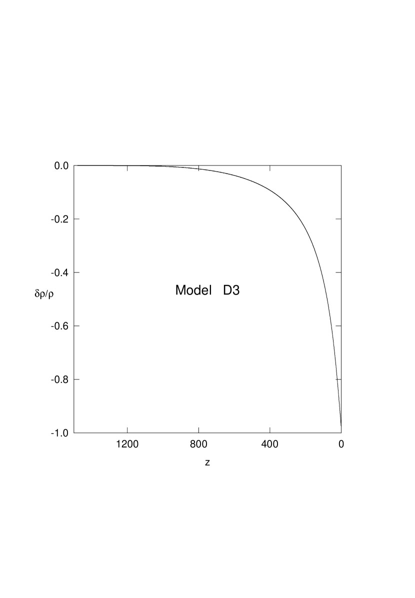
Figure 1: $\delta\rho/\rho$ as a function of redshift.

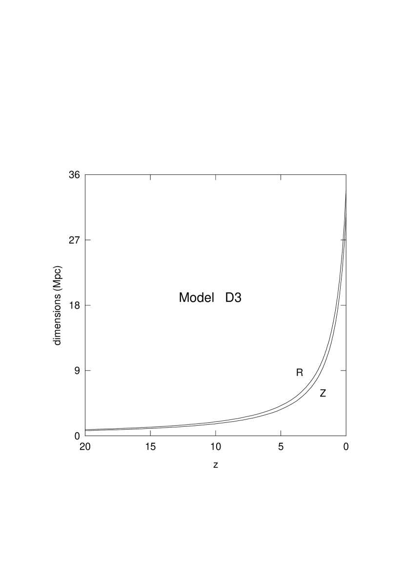
Figure 2: Equatorial (R) and Polar (Z) radii as a function of redshift.

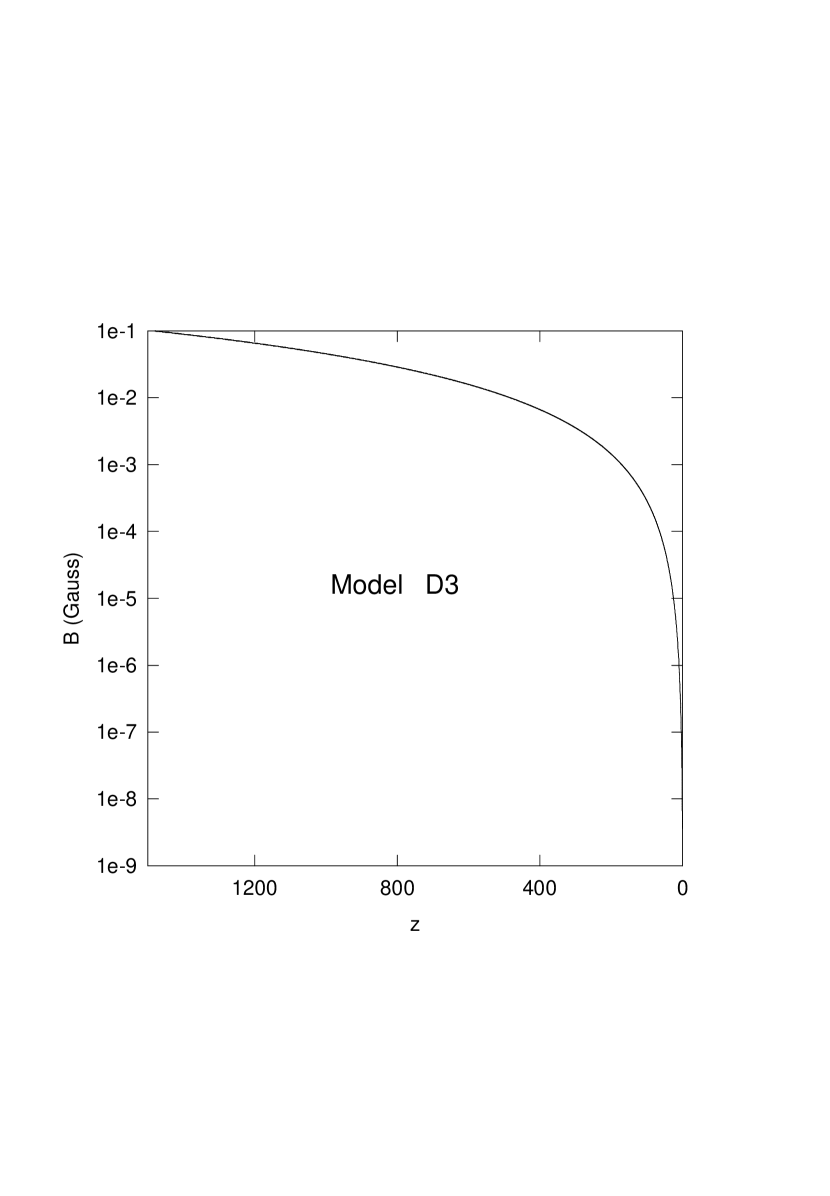
Figure 3: The evolution of the magnetic field as a function of redshift.

References

- Battaner et al. (1996) Battaner, E., Florido, E., and Jiménez-Vicente, J. 1996, astro-ph/9602197
- Cheng et al. (1994) Cheng, B., Schramm, D.N., and Truran, J.W. 1994, Phys. Rev. D, 49, 5006
- da Costa et al. (1994) da Costa, L.N. et al. 1994, ApJ, 424, L1
- de Araujo and Opher (1989) de Araujo, J.C.N. and Opher, R. 1989, MNRAS, 231, 923
- de Araujo and Opher (1990) de Araujo, J.C.N. and Opher, R. 1990, ApJ, 350, 502
- de Araujo and Opher (1991) de Araujo, J.C.N. and Opher, R. 1991, ApJ, 379, 461
- de Araujo and Opher (1993) de Araujo, J.C.N. and Opher, R. 1993, ApJ, 403, 26
- de Araujo and Opher (1994) de Araujo, J.C.N. and Opher, R. 1994, ApJ, 437, 556
- El-Ad el al. (1996) El-Ad, H., Piran, T., and Da Costa, L.N. 1996, ApJ(in press)
- Ge and Owen (1993) Ge, J.P. and Owen, F.N. 1993, AJ, 105, 778
- Grasso nd Rubinstein (1996) Grasso, D., and Rubinstein, H. 1996, astro-ph/9602055
- Harrison (1973) Harrison, E.R. 1973, MNRAS, 165, 185
- Holcomb (1990) Holcomb, K.A. 1990, ApJ, 362, 381
- Kosowsky and Loeb (1996) Kosowsky, A., and Loeb, A. 1996, astro-ph/9601055
- Kronberg (1994) Kronberg, P.P. 1994, Rep. Prog. Phys., 57, 325
- Kronberg et al. (1990) Kronberg, P.P., Perry, J.J. and Zukowsky, E.L.H. 1990, ApJ, 355, L31
- Mestel (1965) Mestel, L. 1965, QJRAS, 6, 265
- Peebles (1968) Peebles, P.J.E. 1968, ApJ, 153, 1
- Peebles (1993) Peebles, P.J.E. 1993, Principles of Physical Cosmology (Princeton University Press)
- Quashnoc et al. (1989) Quashnoc, J.M., Loeb, A., and Spergel, D.N. 1989, ApJ, 344, L49
- Ratra (1992) Ratra, B. 1992, ApJ, 391, L1
- (22) Vainshtein, S.I. and Ruzmaikin, A.A. 1972a, Soviet Ast., 15, 714
- (23) Vainshtein, S.I. and Ruzmaikin, A.A. 1972b, Soviet Ast., 16, 365
- Vallee (1990) Vallee, J.P. 1990, ApJ, 360, 1
- Zweibel (1988) Zweibel, E.G. 1988, ApJ, 329, L1