Non-parametric Reconstruction of Cluster Mass Distribution from Strong Lensing: Modelling Abell 370

Abstract

We describe a new non-parametric technique for reconstructing the mass distribution in galaxy clusters with strong lensing, i.e., from multiple images of background galaxies. The observed positions and redshifts of the images are considered as rigid constraints and through the lens (ray-trace) equation they provide us with linear constraint equations. These constraints confine the mass distribution to some allowed region, which is then found by linear programming. Within this allowed region we study in detail the mass distribution with minimum mass-to-light variation; also some others, such as the smoothest mass distribution.

The method is applied to the extensively studied cluster Abell 370, which hosts a giant luminous arc and several other multiply imaged background galaxies. Our mass maps are constrained by the observed positions and redshifts (spectroscopic or model-inferred by previous authors) of the giant arc and multiple image systems. The reconstructed maps obtained for $A370$ reveal a detailed mass distribution, with substructure quite different from the light distribution. The method predicts the bimodal nature of the cluster and that the projected mass distribution is indeed elongated along the axis defined by the two dominant cD galaxies. But the peaks in the mass distribution appear to be offset from the centres of the cDs.

We also present an estimate for the total mass of the central region of the cluster. This is in good agreement with previous mass determinations. The total mass of the central region is $M=2.0\!-\!2.7\times 10^{14}M_{\odot}h_{50}^{-1}$, depending on the solution chosen.

1 Introduction

Gravitational lensing operates on all scales and provides the best way to reconstruct mass distribution, without any prior hypothesis about the cluster dynamics or mass-to-light ratio, on large scales from 100 kpc to a few Mpc; i.e., from the innermost regions to the far outskirts of clusters. Modelling of clusters with giant arcs directly confirms that their innermost regions are dominated by dark matter and thus plays an important role in probing the distribution of the dark matter in rich clusters.

In the present paper, we describe a new method for reconstructing the cluster Abell 370 [hereafter $A370$] non-parametrically, using the observational constraints provided by strong lensing. It is similar to the method described in Saha & Williams 1997 for galaxy-lenses, and here we develop it for cluster-lenses. To our knowledge, our technique is the first of its kind. The only ingredients needed for our reconstruction are the positions of the multiple images, their redshifts, the luminosity map of the lensing cluster and its redshift. The positions of the images are taken as rigid constraints while the luminosity distribution is a loose constraint subordinate to the lensing data. The model strikingly predicts the observed parameters associated with each image, the ellipticities and orientations. The reconstructed mass distribution compares favourably with the ROSAT/HRI X-ray map which is also bimodal, and moreover almost all major peaks visible in our reconstructed mass map coincide with the X-ray peaks.

Abell 370 is a very rich cluster of galaxies at redshift $z_{\rm cl}=0.375$ and its centre appears to be dominated by two bright cD galaxies, which are, together with their associated dark matter, mostly responsible for the lensing. The two cD galaxies are visible on both the optical ground-based CCD images and the HST WFC-1 image. It was just over a decade ago that $A370$ was first recognised as a lens (Lynds and Petrosian 1986). This was confirmed by the redshift measurement of the observed giant blue arc, $z_{\rm arc}=0.724$ (Mellier et al 1988, Soucail et al 1988).

The giant blue luminous arc, the numerous arc(lets) and the multiple images observed in $A370$, distinguish the cluster and have made it a target for extensive studies, observations and modelling (Soucail et al 1987, Narasimha & Chitre 1988, Kovner 1989, Grossman & Narayan 1989 and Kneib et al 1993 [hereafter K93]). K93, from their superb ground-based CCD image, presented clear evidence that the giant arc consists of at least three multiple merging images, characterising it as a cusp-arc. They presented a fit for the cluster-lens, with the giant arc as three merging images, assuming a bimodal mass distribution calibrated with the giant arc’s redshift and parameterised by the ellipticities and orientations of the two dominant cD galaxies. Such simple mass models may ignore substructures in the cluster mass map, leading to imprecise inversion for determining the redshifts of the background images (Kneib et al 1996). However, their model-inferred redshifts for some of the multiple images were subsequently confirmed by spectroscopy (J. Bezecourt, personal communication).

The remarkable structure of the giant arc in $A370$ and its eastern kink (see below) suggests that the source is straddling a caustic and exhibits a higher order catastrophe than a cusp catastrophe. Careful inspection of the HST image revealed that there are more than two breaks within the arc and tiny elongated bright knots or granules along the arc, which indicates immediately that the arc is, in fact, five merging segments. The K93 model reproduced only the central three parts as multiple images while the two other segments emerge as single images of part of the source. Smail et al 1996, from their HST observations of the giant arc, detected a possible bulge and faint spiral structures visible on the eastern kink. Thus, they claim that the source is a late spiral, which is consistent with the spectroscopic identification. Another feature visible on the HST WFC-1 image is the radial arc $R$, which comprises two merging images across the inner critical curve.

Previous models for $A370$ assume a predefined mass distribution for the cluster, usually based on the parameters of the two dominant cD galaxies, i.e., model $A370$ as a bimodal cluster. The free parameters used in characterising each clump are core radii, ellipticity and orientation. Such a rigid way of modelling may put the resultant mass distribution into a corner of the model space allowed by observations. Thus, simple mass models based only on the observed parameters of the two dominant galaxies may be inaccurate even though they reproduce the multiple images correctly.

The structure of this paper is as follows. In section 2, we describe the basic lensing equations used in modelling the cluster potential and the bending angles. Sections 3 and 4 are devoted to the cluster mass reconstruction, and to testing the robustness of the method, respectively. Explicit use of Fermat’s principle to reproduce the exact location of the multiple images and to test the code is explained in section 5, which also discusses individually all the image systems used in our reconstruction. A final discussion is given in section 6. We take $\Omega_{0}=1$ and $\Lambda=0$ throughout.

2 The Method

The main observables in any lensed system are the image positions, relative magnifications for multiple images if any, the source redshifts, and the lens redshift. If the images are resolved, image ellipticities and orientations are also observable. In this section we develop a method for reconstructing the mass distribution of the lens using constraints provided by (a) the positions of multiple images, (b) image orientations and (c) image ellipticities, given the lens and source redshifts. However, the reconstruction carried out in the present paper uses only the multiple-image positions.

2.1 Pixellated mass distributions

For a source at unlensed angular position $\beta$ the time delay is

$$T(\mbox{\boldmath$\theta$}) = {1+z_{\rm L}\over c}\bigg{(}{D_{\rm L}D_{\rm S}\over 2D_{\rm LS}}(\mbox{\boldmath$\theta$}-\mbox{\boldmath$\beta$})^{2}$$ (2.1)

$$-{4G\over c^{2}}\int\!\Sigma(\mbox{\boldmath$\theta$}^{\prime})\ln|\mbox{\boldmath$\theta$}-\mbox{\boldmath$\theta$}^{\prime}|\,d^{2}\mbox{\boldmath$\theta$}^{\prime}\bigg{)},$$

where $\Sigma(\mbox{\boldmath$\theta$}^{\prime})$ is the surface mass density in the lens plane at a position $\mbox{\boldmath$\theta$}^{\prime}$. Since $z_{\rm L}$ and $D_{\rm L}$ are fixed for a given cluster, we may as well work with a scaled time delay

$$\tau(\mbox{\boldmath$\theta$})={\mathchoice{\hbox{$1\over 2$}}{{1\over 2}}{\scriptstyle{1\over 2}}{1\mskip-1.5mu/\mskip-1.5mu2}}(\mbox{\boldmath$\theta$}-\mbox{\boldmath$\beta$})^{2}-{D_{\rm LS}\over D_{\rm S}}{1\over\pi}\int\!\sigma(\mbox{\boldmath$\theta$}^{\prime})\ln|\mbox{\boldmath$\theta$}-\mbox{\boldmath$\theta$}^{\prime}|\,d^{2}\mbox{\boldmath$\theta$}^{\prime}$$ (2.2)

where

$$\sigma(\mbox{\boldmath$\theta$})={\Sigma(\mbox{\boldmath$\theta$})\over\Sigma_{\rm crit}},\quad\Sigma_{\rm crit}={c^{2}\over 4\pi G}D_{\rm L}.$$ (2.3)

Note that the critical density $\Sigma_{\rm crit}$ as defined in (2.3) is for a source at infinity; hence the factor of $D_{\rm LS}/D_{\rm S}$ in (2.2).

We now consider a pixellated mass distribution for the cluster, with $\sigma_{mn}$ denoting the surface density of the $mn$-th pixel in units of $\Sigma_{\rm crit}$. If $a$ is the pixel size, the total mass is

$$a^{2}\Sigma_{\rm crit}\sum_{mn}\sigma_{mn}.$$ (2.4)

Defining

$$\psi_{mn}(\mbox{\boldmath$\theta$})\equiv{1\over\pi}\int_{mn}\ln|\mbox{\boldmath$\theta$}-\mbox{\boldmath$\theta$}^{\prime}|\,d^{2}\mbox{\boldmath$\theta$}^{\prime}$$ (2.5)

with the integral covering only the $mn$-th pixel, we can write the scaled time delay (2.2) as

$$\tau(\mbox{\boldmath$\theta$})={\mathchoice{\hbox{$1\over 2$}}{{1\over 2}}{\scriptstyle{1\over 2}}{1\mskip-1.5mu/\mskip-1.5mu2}}(\mbox{\boldmath$\theta$}-\mbox{\boldmath$\beta$})^{2}-{D_{\rm LS}\over D_{\rm S}}\sum_{mn}\sigma_{mn}\psi_{mn}(\mbox{\boldmath$\theta$}).$$ (2.6)

Defining

$$\mbox{\boldmath$\alpha$}_{mn}(\mbox{\boldmath$\theta$})\equiv\mathchoice{\partial\over\partial\mbox{\boldmath$\theta$}}{\partial/\partial\mbox{\boldmath$\theta$}}{\partial/\partial\mbox{\boldmath$\theta$}}{\partial/\partial\mbox{\boldmath$\theta$}}\psi_{mn}(\mbox{\boldmath$\theta$})$$ (2.7)

and using Fermat’s principle, i.e images are formed at the extrema of time delay $\nabla_{\mbox{\boldmath$\theta$}}\tau(\mbox{\boldmath$\theta$})=0$, leads to the lens equation

$$\mbox{\boldmath$\theta$}-\mbox{\boldmath$\beta$}={D_{\rm LS}\over D_{\rm S}}\sum_{mn}\sigma_{mn}\mbox{\boldmath$\alpha$}_{mn}(\mbox{\boldmath$\theta$}).$$ (2.8)

Further defining

$$\kappa_{mn}(\mbox{\boldmath$\theta$}) \equiv \frac{1}{2}\left(\mathchoice{\partial^{2}\over\partial\theta_{x}^{2}}{\partial^{2}/\partial\theta_{x}^{2}}{\partial^{2}/\partial\theta_{x}^{2}}{\partial^{2}/\partial\theta_{x}^{2}}+\mathchoice{\partial^{2}\over\partial\theta_{y}^{2}}{\partial^{2}/\partial\theta_{y}^{2}}{\partial^{2}/\partial\theta_{y}^{2}}{\partial^{2}/\partial\theta_{y}^{2}}\right)\psi_{mn}(\mbox{\boldmath$\theta$}),$$ (2.9)

$$\gamma_{mn}(\mbox{\boldmath$\theta$}) \equiv \frac{1}{2}\left(\mathchoice{\partial^{2}\over\partial\theta_{x}^{2}}{\partial^{2}/\partial\theta_{x}^{2}}{\partial^{2}/\partial\theta_{x}^{2}}{\partial^{2}/\partial\theta_{x}^{2}}-\mathchoice{\partial^{2}\over\partial\theta_{y}^{2}}{\partial^{2}/\partial\theta_{y}^{2}}{\partial^{2}/\partial\theta_{y}^{2}}{\partial^{2}/\partial\theta_{y}^{2}}\right)\psi_{mn}(\mbox{\boldmath$\theta$}),$$ (2.10)

$$\delta_{mn}(\mbox{\boldmath$\theta$}) \equiv \mathchoice{\partial^{2}\over\partial\theta_{x}\theta_{y}}{\partial^{2}/\partial\theta_{x}\theta_{y}}{\partial^{2}/\partial\theta_{x}\theta_{y}}{\partial^{2}/\partial\theta_{x}\theta_{y}}\psi_{mn}(\mbox{\boldmath$\theta$}),$$ (2.11)

and

$$H_{mn}(\mbox{\boldmath$\theta$})=\left(\begin{array}[]{cc}\kappa_{mn}+\gamma_{mn}&\delta_{mn}\\ \delta_{mn}&\kappa_{mn}-\gamma_{mn}\end{array}\right)$$ (2.12)

puts the inverse amplification matrix in the form

$$A^{-1}(\mbox{\boldmath$\theta$})=\left(\begin{array}[]{cc}\tau_{xx}&\tau_{xy}\\ \tau_{yx}&\tau_{yy}\end{array}\right)={\bf 1}-{D_{\rm LS}\over D_{\rm S}}\sum_{mn}\sigma_{mn}H_{mn}(\mbox{\boldmath$\theta$}),$$ (2.13)

where $\tau_{xx}=\tau_{\theta_{x}\theta_{y}}$ and so on.

The quantity $\psi_{mn}(\mbox{\boldmath$\theta$})$ is the contribution of the $mn$-th pixel to the potential at $\theta$; similarly $\mbox{\boldmath$\alpha$}_{mn}(\mbox{\boldmath$\theta$})$ is the $mn$-th pixel’s contribution to the bending angle, and the second derivatives are contributions to terms in the inverse amplification matrix.

In this paper we will consider square pixels. We have also experimented with pixels that are Gaussian circles with overlapping tails. Gaussian pixels avoid discontinuities in the mass that square pixels imply, but the difference in the final results is very small. This is because the bending angle integrates once over the mass distribution and the potential integrates twice, which tends to wash out any effects of mass discontinuities at pixel boundaries.

Explicit expressions for $\psi_{mn}(\mbox{\boldmath$\theta$})$ and its derivatives for square pixels are given in Appendix A.

2.2 Constraint equations and inequalities

Since $\psi_{mn}(\mbox{\boldmath$\theta$})$ and its derivatives are known functions, the lens equation (2.8) and the inverse amplification (2.13) are linear in $\sigma_{mn}$ and $\beta$, i.e. the unknowns that the reconstruction method must infer. This linearity renders multiple-image positions, orientations and ellipticities into linear constraints on the pixellated mass distribution.

First consider multiple images. For each image, we write the lens equation (2.8) at the observed $\theta$ and thus get a two-component constraint equation. But each source $\beta$ introduces two extra numbers to solve for, so multiple image systems actually supply $\rm 2(\langle{images}\rangle-\langle{sources}\rangle)$ constraints.

Orientations and ellipticities of single but distorted images can also provide linear constraints. Suppose we have an image at $\theta$ observed elongated along position angle $\phi$, and consider the inverse amplification matrix in coordinates $\theta_{x}^{\prime},\theta_{y}^{\prime}$, rotated by $\phi$. We will have

$$A^{-1}=\left(\begin{array}[]{cc}\tau_{x^{\prime}x^{\prime}}&\tau_{x^{\prime}y^{\prime}}\\ \tau_{y^{\prime}x^{\prime}}&\tau_{y^{\prime}y^{\prime}}\end{array}\right).$$ (2.14)

having the same form as in equation (2.13) but with $H_{mn}(\mbox{\boldmath$\theta$})$ replaced by its rotated version:

$$\left(\begin{array}[]{cc}\kappa_{mn}+c\gamma_{mn}+s\delta_{mn}&-s\gamma_{mn}+c\delta_{mn}\\ -s\gamma_{mn}+c\delta_{mn}&\kappa_{mn}-c\gamma_{mn}-s\delta_{mn}\end{array}\right)$$ (2.15)

where $c$ stands for $\cos 2\phi$ and $s$ stands for $\sin 2\phi$. Since $\phi$ is known (because measured from the observed image), $A^{-1}$ in equation (2.14) is linear in $\sigma_{mn}$. Consider an image that appears more elongated than what is expected based on the intrinsic ellipticity distribution of galaxies, but does not look like an edge-on spiral. With a rough estimate of the galaxy’s redshift, and assuming that galaxy’s intrinsic ellipticity is aligned with its lensing-induced elongation, we can infer that its magnification along the $\theta_{x^{\prime}}$ direction is at least $k$ times that along the perpendicular direction. In such a case we can write

$$k|\tau_{x^{\prime}x^{\prime}}|\leq|\tau_{y^{\prime}y^{\prime}}|.$$ (2.16)

This becomes a linear constraint on the $\sigma_{mn}$ if we can infer the image parity from a rough idea of where the critical curves are, and thus remove the absolute value signs. In cases where we can confidently assert that (say) the magnification along $\theta_{x^{\prime}}$ is at least $k$ in absolute value, we can write

$$-1/k\leq\tau_{x^{\prime}x^{\prime}}\leq 1/k;$$ (2.17)

and here the parity doesn’t matter. Finally, for very large distortions where it is clear that the amplification eigenvectors are along $\theta_{x^{\prime}}$ and $\theta_{y^{\prime}}$ we can write

$$\tau_{x^{\prime}y^{\prime}}=0;$$ (2.18)

here again parity doesn’t matter.

Notice that the constraint (2.16), usually with an equality sign, is the type of information that weak lensing observations provide. Because weak lensing generally produces mild ellipticity changes, many galaxy images have to be averaged over to suppress the noise due to intrinsic galaxy ellipticities and enhance the lensing signal. The same procedure can be applied in our case using average magnifications in (2.16), instead of magnification of individual galaxies. This opens up the possibility of combining strong and weak lensing data in a mass reconstruction. In this paper we will explore only the multiple-image constraints and leave ellipticities and orientations for future work.

2.3 Producing a mass map

The various observational constraints above, combined of course with

$$\sigma_{mn}\geq 0,$$ (2.19)

confine the pixellated mass distribution to some allowed region. Since the constraints are all linear, it is straightforward to find this allowed region by linear programming. But since the number of pixels will in practice far exceed the number of constraints, the allowed region will contain a vast family of mass distributions, all consistent with the observations. To obtain mass maps, we need to add more information.

There are several standard ways of adding and justifying the extra information. For example, we could ask for the smoothest mass distribution consistent with the data, or for a maximum entropy distribution. But for this problem, a different figure of merit seems more appropriate: since one of the aims of cluster mass reconstruction is to test how well light traces mass, it is interesting to study the mass distribution that follows the light as closely as the lensing data allow. We can think of this as a ‘minimum $M/L$ variation’ mass map. We have found that this criterion by itself tends to produce artifacts on small scales, so we include a term that tends to smooth over the mass distribution on short scales. More precisely, our mass maps minimise $\Delta^{2}$ subject to the linear lensing constraints, where

$$\Delta^{2} = \sum_{mn}\left(\sigma_{mn}-L_{mn}{\textstyle\sum_{kl}\sigma_{kl}}\right)^{2}$$ (2.20)

$$+ \epsilon^{4}a^{-4}\sum_{mn}(\sigma_{m+1,n+1}+\sigma_{m-1,n-1}+$$

$$\sigma_{m+1,n-1}+\sigma_{m-1,n+1}-4\sigma_{mn})^{2}.$$

In equation (2.20), $L_{mn}$ is the light associated with the $mn$-th mass pixel, scaled so that $\sum_{mn}L_{mn}=1$. The first term in $\Delta^{2}$ thus tends to minimise mass-to-light variations. The second term in $\Delta^{2}$ is a discrete version of $\epsilon^{4}\int\!(\nabla^{2}\sigma)^{2}$; minimizing the integrated square of second derivative is one way of smoothing. As before, $a$ is the pixel size, so $\epsilon$ can be interpreted as a smoothing scale.

The numerical problem we now have to solve is to find the minimum of a quadratic function of the $\sigma_{mn}$ (i.e., $\Delta^{2}$) subject to linear equality and inequality constraints involving the $\sigma_{mn}$. This type of problem is known as quadratic programming. If there is a solution, it is unique and subroutines for finding it are widely available. We used the NAG routine E04NFF. The technique is limited by storage rather than speed: for $N$ pixels the storage required is $\simeq 2N^{2}$. So a few thousand pixels is the current limit.

3 The Lens Reconstruction

The cluster $A370$ ($z_{\rm cl}=0.375$, corresponding to $D_{\rm L}=6.1\rm\,kpc\,arcsec^{-1}$), hosts not only the first detected giant arc but also several multiple resolved images and weakly distorted arclets (Fort et al 1988, K93). In this paper we will consider only multiply imaged systems, which are in a field of $2^{\prime}\times 2^{\prime}$. We take the image positions from the recent HST images of $A370$ (Smail et al 1996) and the redshifts from K93; these are tabulated in Table 1 and illustrated on Fig. 1. The critical surface mass density for sources at infinity is $5.04\times 10^{10}h_{50}^{-1}M_{\odot}arcsec^{-2}$.

Figure 1: Multiple images systems in the cluster $A370$.

The results we describe in this paper use pixel size $a=2.1^{\prime\prime}$; experiments with other pixel sizes indicated little sensitivity to $a$.

3.1 Observational constraints

As explained in Section 2.2, each image contributes two linear constraint equations but each source adds two new quantities to solve for, and hence the number of constraints on the mass distribution is $2\rm(\langle{images}\rangle-\langle{sources}\rangle)$.

System	Images		$x$(arcsec)		$y$(arcsec)
$A0$	Giant arc
$(z=0.724)$	P1		$-13.58$		$-18.53$
	P2		$-8.05$		$-20.27$
	P3		$-3.40$		$-20.76$
	P4		$1.75$		$-19.30$
	P5		$6.11$		$-16.96$
$B$
$(z=0.806)$	B2		$2.43$		$9.41$
	B3		$7.76$		$8.92$
	B4		$-24.62$		$9.22$
$C$
$(z=0.810)$	C1		$0.68$		$-4.75$
	C2		$4.27$		$-6.31$
$R$	Radial arc
$(z=1.3)$	R1		$-0.49$		$-4.17$
	R2		$-0.79$		$-5.36$
$A1$
$(z\simeq 1.2)$	S1		$-0.10$		$47.72$
	S2		$1.46$		$47.43$
$A13$
$(z=1.7\pm 0.2)$	Q1		$53.06$		$21.05$
	Q2		$52.38$		$22.41$

Table 1: Positions of the various sets of image system as taken from the HST images.

• The giant arc $A0$ at $z_{A0}=0.724$ (Soucail et al 1987), with its eastern kink, was modelled by K93 as multiple merging images of a single background source. However, the identification of the multiple images is somewhat complex and uncertain. For example, in K93 only the central part is multiply imaged. From inspection of the HST image it seems plausible that the giant arc is a five image-system, and this is the interpretation we follow in this paper. However, we found that a three-image interpretation gave a very similar lens reconstruction. This system supplies 8 constraints.

• The $B2$-$B3$ and $B4$ images at $z_{B}=0.806$ (J. Bezecourt private communication), which is close to the model-inferred value of 0.865 in Kneib et al (1994 [hereafter K94]), are identified as multiple images of a single source, and thus they provide 4 constraints.

• The faint pair $C1$-$C2$ at $z_{C}=0.810$ (K93, K94) contributes 2 constraints.

• The recently identified radial arc $R$ at $z_{R}=1.3\pm 0.2$, (Smail et al 1996) on the HST images consists of two main elongated segments, in which a few bright granules separated by sub-arcseconds are visible. Again we face here the uncertainty in image identification, and we take only the position of the two main segments. Hence, the radial arc provides us with 2 more constraints.

Most of the image systems considered above are located in the innermost regions of the cluster and thus will constrain mostly the region they lie in. We added a few more constraints from images further out in the cluster, but still lying within in our field. We included the arclets $A1$ and $A13$:

• The arclet $A1$ at $z_{A1}\approx 1.2$ (K94) is a two-component distorted image, $S1$-$S2$, and adds 2 more constraints.

• The arclet $A13$ at $z_{A13}=1.7_{-0.15}^{+0.1}$ (K94) is also a two-component distorted image, $Q1-Q2$, and provides 2 extra constraints.

The total from all the above image systems is 20 constraints.

Table 2: Fiducial parameters of lensing galaxies used in our reconstruction. (Note that some galaxies have centroids outside our $2^{\prime}\times 2^{\prime}$ field, but are included here because their wings extend into our field.) The numbering and $B$ magnitudes are taken from Mellier et al. 1989. The two cD galaxies in this cluster are #20 & #35.

FIDUCIAL PARAMETERS OF A370 MEMBERS

	MSFM No.		$x{\rm(arcsec)}\pm 0.2$		$y{\rm(arcsec)}\pm 0.2$		$B$
	7		$23.8$		$63.5$		22.22
	8		$11.5$		$63.3$		21.91
	9		$-2.4$		$62.2$		21.25
	10		$-31.1$		$65.1$		20.13
	12		$18.5$		$43.1$		20.86
	13		$22.8$		$53.1$		21.80
	14		$44.3$		$48.0$		21.69
	15		$56.0$		$67.8$		19.68
	16		$39.3$		$51.1$		22.52
	17		$-41.6$		$35.2$		21.39
	18		$-47.2$		$20.9$		20.98
	20		$-2.8$		$25.5$		20.40
	21		$-1.3$		$19.5$		21.01
	23		$56.6$		$15.6$		21.07
	28		$20.7$		$-5.0$		21.09
	29		$-20.5$		$6.7$		22.82
	30		$-30.0$		$1.8$		22.19
	31		$-53.4$		$5.7$		21.85
	32		$-55.2$		$10.8$		20.44
	34		$-39.9$		$-4.0$		21.49
	35		$-5.3$		$-11.3$		20.93
	36		$-56.4$		$-24.2$		21.90
	37		$-8.2$		$-18.9$		21.51
	52		$10.4$		$25.9$		21.85
	54		$-32.5$		$46.5$		21.64
	56		$-19.9$		$-24.9$		22.04
	58		$15.4$		$-34.6$		21.10

3.2 Pixellated light map

Figure 2: Luminosity map of the cluster $A370$. Filled numbered circles mark the positions of galaxies used to produce the map. The numbering of the galaxies follows Mellier et al 1988.

The pixellated light distribution of the cluster-lens $A370$ is based on Mellier et al 1988. We used the apparent magnitudes of 27 individual galaxies, including the two dominant cD galaxies [see Table 2], to obtain a smoothed luminosity map. Each of the 27 galaxies is replaced by a Gaussian light profile of dispersion $\theta_{g}=8^{\prime\prime}$

$$L_{mn}\propto\sum_{j=1}^{27}10^{-0.4m_{j}}\exp\left(-(\mbox{\boldmath$\theta$}_{mn}-\mbox{\boldmath$\theta$}_{j})^{2}\over 2\theta_{g}^{2}\right),$$ (3.21)

where $m_{j}$ is the apparent magnitude of the $j$th galaxy and $\mbox{\boldmath$\theta$}_{j}$ is the location of the $j$-th galaxy. This smoothed luminosity is plotted in Fig. 2.

3.3 Minimum $M/L$ variation: ML model

Now we have all the necessary ingredients to reconstruct the cluster mass distribution that follows the light as closely (in the least-squares sense) as the lensing data allow. We also have the option of smoothing the mass distribution at various small scales $\epsilon$ (see Eq. [2.20]) while still satisfying the lensing data.

Figure 3: Our best reconstructed mass distribution of the cluster $A370$. The cluster is clearly bimodal, with the two most massive clumps in the central region close to two cD galaxies (marked with +) in this cluster, but slightly closer together than the visible galaxies. The dashed rectangle encloses the region where we consider the mass reconstruction to be most robust. The contour lines are annotated in steps of $0.25\times\Sigma_{\rm crit}$. In all the following mass maps we adopt the same contour levels.

Our reconstructed mass distribution for smoothing parameter $\epsilon=3.5^{\prime\prime}$ is presented in Fig. 3. Figure 4 shows reconstructions with other values of $\epsilon$. All the reconstructions satisfy the lensing constraints precisely, but we found that $\epsilon=3.5^{\prime\prime}$ is the lowest value that eliminates evident small-scale artifacts, and in the rest of this paper we will mainly discuss this case.

As in K93 our mass reconstruction shows bimodality in the cluster, and this persists on mass maps for different values of $\epsilon$—see Fig. 4. However, our non-parametric reconstruction shows details of this bimodality not seen in previous work. First, the centres of the two dominant mass clumps do not coincide with the two dominant cD galaxies, but are slightly closer together, roughly along the line joining the two cDs. Second, the southern clump is much more massive than the northern clump, although the northern cD galaxy is brighter. Third, the mass distribution reveals extra substructure in the innermost regions of the cluster, between the two cDs. Some of these extra substructures are not associated with light, but are required by the lensing data, while some are in the vicinity of cluster galaxies which did not make it into the Mellier et al 1989 classification scheme, and so were not included in our isoluminosity profile, but again our model predicts their requirement by the lensing data. Thus our non-parametric model indicates that there is a substantial amount of dark matter in the innermost regions of $A370$, which does not closely follow the distribution of light.

Figure 4: The reconstructed mass distribution using various values for the smoothing scale factor $\epsilon$. It is very reassuring that the bimodality is preserved for the different values of $\epsilon$.

Comparison of ROSAT/HRI X-ray map (as seen in Fort & Mellier 1994, Mellier et al 1994) and our reconstructed maps reveals very similar morphologies. Reassuringly, it reveals a coincidence of the two main central clumps that are associated with the two giant cD galaxies. Moreover, on larger scales the X-ray map shows an elongation towards the region of arclet $A1$ as well as secondary peaks in north-east direction, which are well matched by peaks in our reconstructed maps. This close similarity between the ROSAT/HRI X-ray map for $A370$ and our reconstructed maps, even on larger scales, supports the results of our lens modelling.

3.4 Maximally flat model: MF model

To see whether minimizing $M/L$ variation was introducing large biases into the reconstruction, we generated another reconstruction, which we call the MF model, with

$$L_{mn}={\rm const}.$$ (3.22)

The resulting mass distribution, presented in Fig. 5, is the map with the minimum dispersion in mass that still reproduces the image positions. It is reassuring to see that in this case, we still recover the main features of the minimum $M/L$ variation mass map, most importantly, the bimodal nature of the cluster. Comparing maps of Figs. 3 and 5, we see that even some smaller features are reproduced in both maps.

Figure 5: The reconstructed mass distribution using uniform $L_{mn}$, which reveals the bimodal nature of the cluster.

3.5 Uncertainties in redshifts

Of the various multiple image systems in A370, only $A0$ and $B$ have spectroscopic redshifts; as noted in 3.1, the redshifts of the other systems are model-inferred (K93 & K94). To test whether our reconstructions are sensitive to these redshifts, and hence to model dependencies in the K93 and K94 work, we generated some more ML maps where the model-inferred redshifts are swapped around. The swapping $z_{C}\to z_{R}\to z_{C}$ and $z_{C}\to z_{R}\to z_{A13}\to z_{C}$ both produced maps that preserved bimodality as well as most of the extra substructures in inner regions of the cluster; however we noticed that more mass tends to be put in the vicinity of high redshift images. The permutation $z_{C}\to z_{A13}\to z_{R}\to z_{C}$ yielded no feasible solution; our interpretation is that if $z_{A13}$ becomes too low, it is impossible to make the $A13$ images far enough apart without inconsistencies with data on other images.

We thus conclude that our reconstructions are only weakly sensitive to uncertainties in the model-inferred redshifts used.

More tests of the robustness of our reconstructions are described in the next section.

3.6 Mass estimates

Our reconstructions provide mass estimates for the whole field, but as we saw above, the mass is well constrained only in the central region, where most of the multiple-image systems lie. Table 3 lists our mass estimates for the central $45^{\prime\prime}\times 65^{\prime\prime}$ region (enclosed by a dashed rectangle in Fig. 3 for the ML, MF and mean RL (see next section) cases, along with previous estimates from the literature. From our different reconstructions, we conclude that

$$M_{45^{\prime\prime}\times 65^{\prime\prime}}=(2.3\pm 0.3)h_{50}^{-1}\times 10^{14}M_{\odot}.$$ (3.23)

Table 3: Previously published mass estimates of the central region of the cluster compared with our estimates. Our estimates refer to the $45^{\prime\prime}\times 65^{\prime\prime}$ region within the dashed rectangle in Fig. 3. Previous workers have usually given mass estimates within a critical radius, so the regions considered are not precisely equivalent.

Model	$10^{14}h_{50}^{-1}M_{\odot}$
Hammer 1987	2.
Soucail et al 1987	2.
Narasimha & Chitre 1988	4.2
Grossman & Narayan 1989	0.93
Mellier et al 1990	2.
This work:
ML	2.3 $\pm 0.3$
MF	2.7
RL	2.2 $\pm 0.2$

The mass of the whole $2^{\prime}\times 2^{\prime}$ field is much less well constrained by our reconstructions. The ML model gives

$$M_{2^{\prime}\times 2^{\prime}}\simeq 4.5\times 10^{14}h_{50}^{-1}M_{\odot},$$

while the MF model gives

$$M_{2^{\prime}\times 2^{\prime}}\simeq 6.6\times 10^{14}h_{50}^{-1}M_{\odot}.$$

That the ML estimate should be lower is understandable when we think about what the minimum $\Delta^{2}$ criterion [Eq. (2.20)] does: it follows the lensing requirements in the regions where there are multiple images, elsewhere it tends to extrapolate using the given $L_{mn}$.

4 Testing the Robustness of the method

Figure 6: Some of the reconstructed mass distributions for the RL case (see text); in each case the rotation angle $\phi$ is stated.

In this section we will estimate the robustness of our method. We produce an ensemble of reconstructions, as described below, and calculate the ensemble dispersion in mass as a function of position in the lens plane.

Figure 7: Contours of $\Delta\sigma_{mn}$in the lens plane. The mass distribution is strongly constrained in the central region of the cluster, i.e., region with high number density of images.

For each reconstruction in the ensemble, we derive $L_{mn}$ by rotating the positions of the all the galaxy members by an angle $\phi$ in the lens plane. Let us call these RL, rotated light, reconstructions. Figure 6 shows some of these. As in the ML and MF reconstructions, the main features of the mass map also appear in all the versions of the RL maps. Thus we see the reconstructed mass maps are quite robust, especially in the regions well sampled by the observed images. We will now quantify this statement

From the RL mass distributions, we can readily calculate pixel-by-pixel ensemble means and dispersions. Let us define

$$\Delta\sigma_{mn}=\left[{\langle{\sigma_{mn}^{2}}\rangle\over\langle{\sigma_{mn}}\rangle^{2}}-1\right]^{\mathchoice{\hbox{$1\over 2$}}{{1\over 2}}{\scriptstyle{1\over 2}}{1\mskip-1.5mu/\mskip-1.5mu2}}$$ (4.24)

which is just the ratio of ensemble dispersion to ensemble mean. It quantifies the uncertainties in our reconstruction. Figure 7 shows contours of $\Delta\sigma_{mn}$ in the lens plane. It clearly shows that the reconstructed mass distribution is indeed very well constrained ($\Delta\sigma_{mn}\leq 0.25$) in the inner most regions of the cluster, where almost all the multiple images lie. This implies that the image positions indeed strongly constrain the mass distribution enclosed by them. Moreover, there are two extra regions far from the centre which show some contours revealing constrained mass distributions in their vicinity. These are the two regions with the additional images, $A1$ and $A13$ (see table 1), which we added to constrain the outskirts of the cluster.

Figure 8: A plot of number of images versus $\Delta\sigma_{mn}$, the standard deviation of the reconstructed mass distribution. The solid line connects the average points of $\Delta\sigma_{mn}$ for the corresponding numbers of images, and the dashed line is a fit. Basically the figure shows that regions with more images are well constrained.

Since the observed multiple images are not uniformly sprinkled over the lens plane, the reconstructed mass distribution is not equally well constrained over the whole lens plane; areas with more images are more constrained. In order to visualise this effect, in Fig. 8 we plot the average value of $\Delta\sigma_{mn}$ computed within circles of radius $10^{\prime\prime}$ at a number of arbitrarily placed points in the lens plane, against the number of images inclosed by the circle. Clearly, the robustness of the reconstructed map in the lens plane increases with the number density of images.

5 Discussion of the Various Image Systems

In this section we discuss extensively all the image systems used in our modelling and also examine their predicted shape parameters. We start with the simplest configuration of images.

5.1 B-System

Figure 9: The arrival time contours for set $B$. Filled circles mark the positions of the observed $B2-B3$ and $B4$. The scale shown is in arcseconds.

A good way to verify that our modelling code actually reproduces the observed image positions is to use Fermat’s principle. In Fig. 9 we show a contour plot of the time delay surface for the image set $B$ ($z_{B}=0.806$). The extrema and saddle points of such a surface mark the locations of the images produced by the model and as expected they precisely coincide with the observed positions of $B2$, $B3$ and $B4$. This fit indeed approves of the model. The topography of the arrival time surface for the $B$ image set turns out to be a lemniscate—see Fig. 10a below.

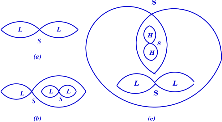
Figure 10: Inferred topological configurations, of the isochronal contours that pass through a saddle point,for the various image sets considered in this paper. Here (a) represents the three-image configuration that corresponds to the $B$, $C$ $A1$ and $A13$ image sets, (b) represents the image configuration of the giant arc $A0$ and (c) represents the interesting seven image-configuration obtained for the radial arc system in some reconstructions—in others the lemniscate with two maxima and a saddle point is replaced by a single maximum.

The small angular separation between the nearly merging pair $B2$-$B3$ and the fact that one is almost a mirror image of the other suggests that a critical curve must be passing between them. We explored critical curves with a recursive code that searches for sign changes, and hence zeros of $\det|A^{-1}(\mbox{\boldmath$\theta$})|$. Figure 11 shows the critical curves for the $B$ system, with the images $B2$, $B3$ and $B4$ also indicated.

Figure 11: The critical curve at $z_{B}=0.806$, with the observed positions of the images $B2$, $B3$ and $B4$ marked by asterisks.

Mapping the critical curves onto the source plane, using the lens equation, gives the caustics. Figure 12 shows the caustics for the $B$ system, with the inferred position of the $B$-source also marked. The position of the $B$ source with respect to the caustics show that it is experiencing a beak-to-beak fold catastrophe.

Figure 12: The caustics at $z_{B}=0.806$, with an asterisk marking the inferred position of the source galaxy $B$.

5.2 C-System, A1 and A13 systems

Figure 13: Time delay contours for the $C$-system and the arclets $A1$ and $A13$. The filled circles marked $C1$ and $C2$ show the corresponding observed image positions and moreover a third image is predicted for the same pair on the other side of the lens major axis. The very top arrival time contour is that of the arclet $A1$ and the one on the far right belongs to the arclet $A13$. Though this figure does not show such detail, these arclets are inferred to be three-image systems too.

The time delay surface for the $C$ system reproduce precisely the observed position of the pair $C1$-$C2$ and also predict a third image located on the other side of the lens major axis (Fig. 13). The predicted position of the third image is in the same location as predicted before by K93 and coincides with a faint blob in the HST image. The topological configuration of the isochrones of the $C$ system is again a lemniscate. The caustics at the predicted $C$ source position also exhibit a beak-to-beak fold catastrophe.

The arclets $A1$ and $A13$ follow the same pattern of the $B$ and $C$ systems and their topological configuration correspond to lemniscates too (see Fig. 10-(a)).

The lensed pair usually denoted as $D1$-$D2$, when we tried including it, gave results similar to those for the $C1$-$C2$ pair. However, we have not included this system in the present paper because its redshift is still uncertain (Kneib 1997, private communication).

5.3 $A0$-System

Figure 14: Time delay contours for the giant arc $A0$. Filled circles mark the observed position of the five segments of $A0$.

Figure 14 shows the time-delay contours for the giant arc $A0$. The extrema and saddle points precisely fit the observed positions of the five segments that constitute the giant arc. The isochrones of this surface correspond to a lemniscate embedded in another lemniscate (Fig. 10-(b)). There is no counter-arc.

Figure 15: The critical curve at $z_{A0}=0.724$. The observed positions of the five segments are marked with asterisks.

Figure 16: The caustics at $z_{A0}=0.724$. The caustic lines in the lower region are shown magnified in an inset. The inferred source position, marked by a filled circle, indicates clearly that the source is exhibiting a catastrophe which is of a higher order than a cusp.

Figures 15 and 16 show respectively the critical curves and caustics at $z_{A0}=0.724$. The lower part of the latter figure reveals a spectacular shape for the cusps. Such cusps are called butterfly cuspoids (Berry & Upstill 1980), and they are a higher-order catastrophe than just a cusp. The predicted position of the $A$ galaxy source is marked by a filled circle on Fig. 16, which crosses the caustic at least twice. These results for the behaviour experienced by the $A$ source galaxy indicates that the giant arc $A0$ may be the result of higher-order catastrophe than just the elementary cusp. If so, it would be the first giant butterfly-cuspoid arc observed.

5.4 $R$-System

Deep HST observations of clusters with spectroscopically confirmed giant arcs has revealed lots of detailed substructures and lensed features which had not been previously detected on ground-based CCD images. The exceptional lensed feature visible on $A370$ HST WFC-1 image (Smail et al 1996) is the radial arc $R$, which does not show up even on the deep CFHT images of the cluster (K93). Close inspection of the radial arc shows some bright blobs within the two main elongated segments. In reconstructing the mass distribution we used only the constraints given by the position of the two main segments, which we call $R1$-$R2$.

Figure 17: Contours of arrival time surface for the radial-arc. The two filled circle, $R1-R2$, mark the position of the two main segments considered in our mass modelling.

¿From the time-delay surfaces, we infer that the $R1$ and $R2$ are two nearby images from a five-image or seven-image system. Two of the images are located on either side of the lens major axis, while the remainder, including $R1$-$R2$, are aligned together with small angular separation close to the southern cD galaxy. Fig. 17 shows the time-delay surface corresponding to Fig. 3, and here the radial arc consists of five aligned images. With Gaussian pixels, the arc was formed out of only three aligned images; the small lemniscate was replaced by a single maximum, but otherwise the time delay surface (and the mass distribution) was very similar. The length of the elongated three- or five-image alignment is about $5.2^{\prime\prime}\pm 0.2^{\prime\prime}$, which exactly fits the observed length of the radial arc.

Figure 18: The critical lines at the redshift of the observed radial arc $z_{R}=1.3$. Filled circles mark the position of the two segments of the radial arc $R1-R2$.

For this particular case, we recall that all our reconstructed mass distributions predict chaotic mass fluctuations between the two cD envelopes and detect the presence of dark sub-clumps closer to the southern cD galaxy. These massive sub-clumps, if taken individually would have their corresponding radial critical curves nearly overlapping (Fig. 18), and hence nearly overlapping radial caustic lines. A single extended source lying in the vicinity of these multi-radial caustics (Fig. 19), will lead to an observation of such image configuration of very close radial arcs.

It is of particular interest to notice the dramatic change of the critical curves and caustics with redshift. (See for example the sequence of Figures 16, 12, 19). Notice the emergence of the radial critical curves and caustics at high redshifts (Fig. 19). These suddenly emerged caustics at high redshift are called lips caustics (see Schneider et al 1992). Since our reconstruction predicts the $R$ source galaxy is straddling these newly formed caustics, we argue that the radial arc is a “lips” arc.

Figure 19: Caustic lines at $z_{R}=1.3$, with the filled circle marking the predicted position of the $R$ source.

Table 4: Shape parameters of various sets of images as predicted by the model. Almost all the parameters, i.e., orientations and ellipticities, predicted by the model are close to the observed ones.

Predicted shape parameters

Source	Images	$\theta$	$e_{1}$	$e_{2}$	$\theta_{\rm obs}$
$A0$	Giant arc
$(z=0.724)$	P1	$-0.276$	$0.030$	$0.612$	$-0.363$
	P2	$-0.231$	$-0.034$	$0.584$	$-0.263$
	P3	$0.077$	$0.025$	$0.625$	$0.000$
	P4	$0.435$	$-0.084$	$0.547$	$0.391$
	P5	$0.705$	$0.317$	$0.770$	$0.708$
$B$
$(z=0.806)$	B2	$0.035$	$-0.227$	$0.400$	$0.000$
	B3	$0.285$	$0.628$	$0.758$	$0.165$
	B4	$-0.077$	$0.518$	$1.059$	$-0.150$
$C$
$(z=0.810)$	C1	$-0.240$	$-0.236$	$0.242$	$-0.175$
	C2	$-0.388$	$0.144$	$0.323$	$-0.450$
$R$	Radial arc
$(z=1.3)$	R1	$-0.191$	$-0.634$	$-0.020$	$-0.192$
	R2	$-0.313$	$-0.628$	$-0.002$	$-0.261$

Almost all the parameters associated with the various images, e.g. amplification, eccentricity, parity and orientation, depend more or less on linear combinations of the second derivatives of the projected potential and the images redshift. Our model predicts these quantities for each individual image and are in good agreement with the observations. Table 4 lists the orientation angle $\theta$ from the horizontal in radians and $e_{1}$ and $e_{2}$, the two eigenvalues of the inverse amplification matrix and their ratio gives the eccentricity. The sign of these eigenvalues specifies the parity of the image; e.g., the image is minimum $L$ if both $e_{1}$ and $e_{2}$ are positive, is a maximum $H$ if both are negative and a saddle $S$ if they have opposite signs.

6 Conclusions

In this paper we have developed a non-parametric technique for reconstructing the mass distribution of galaxy clusters with strong gravitational lensing. We divide the projected lens mass into square pixels, and treat each pixel as an independent contributor to the lensing potential. The observed positions of multiple images provide linear constraints on this pixellated mass distribution. We can then explore the mass distributions that are allowed by these constraints; a particularly interesting model is the one that follows the light as closely as consistency with the lensing data allow.

We applied the new method to the well known cluster Abell 370. The reconstructed mass maps are invariably bimodal. The two largest mass clumps coincide roughly with the two cD galaxies, but are closer together than the visible cD galaxies. Also, though the northern cD galaxy appears to be brighter, our reconstruction reveals that the southern mass clump is much more massive. Our reconstructions also show various other features that may be identified with features on the X-ray map. In the central region, where most of the multiple images are, the mass is well constrained; we estimate the mass of a central $45^{\prime\prime}\times 65^{\prime\prime}$ field as $2.3\pm 0.3\times 10^{14}h^{-1}M_{\odot}$. The mass of the whole $2^{\prime}\times 2^{\prime}$ field is estimated to be 4–6$\times 10^{14}h^{-1}M_{\odot}$.

In addition, we have studied in detail the time delay surfaces, critical curves and caustics for the various multiple image systems in A370. In particular, we argue that the giant arc may be a five-image system at a butterfly cuspoid catastrophe, and that the recently discovered radial arc may be part of a seven-image system at a lips catastrophe.

Appendix A

This Appendix gives expressions for the integral over individual pixels in equation (2.5), and its derivatives. In the following we write $x,y$ for $\theta_{x},\theta_{y}$.

The integrals over pixels are most conveniently evaluated by first considering the corresponding indefinite integrals and then differencing between pixel-corner values. The indefinite integral correspond to equation (2.5) is

$$\tilde{\psi}_{mn}(x,y) = {1\over 2\pi}\bigg{(}x^{2}\arctan{y\over x}+y^{2}\arctan{x\over y}$$

$$+xy\ln(x^{2}+y^{2})-3\bigg{)}.$$

Taking the pixel size as $a$ and noting that the $mn$-th pixel is centred at $(ma,na)$, the desired definite integral is

$$\psi_{mn}(x,y) = \tilde{\psi}_{mn}\left(x-(m+{\mathchoice{\hbox{$1\over 2$}}{{1\over 2}}{\scriptstyle{1\over 2}}{1\mskip-1.5mu/\mskip-1.5mu2}})a,y-(n+{\mathchoice{\hbox{$1\over 2$}}{{1\over 2}}{\scriptstyle{1\over 2}}{1\mskip-1.5mu/\mskip-1.5mu2}})a\right)$$

$$+ \tilde{\psi}_{mn}\left(x-(m-{\mathchoice{\hbox{$1\over 2$}}{{1\over 2}}{\scriptstyle{1\over 2}}{1\mskip-1.5mu/\mskip-1.5mu2}})a,y-(n-{\mathchoice{\hbox{$1\over 2$}}{{1\over 2}}{\scriptstyle{1\over 2}}{1\mskip-1.5mu/\mskip-1.5mu2}})a\right)$$

$$- \tilde{\psi}_{mn}\left(x-(m+{\mathchoice{\hbox{$1\over 2$}}{{1\over 2}}{\scriptstyle{1\over 2}}{1\mskip-1.5mu/\mskip-1.5mu2}})a,y-(n-{\mathchoice{\hbox{$1\over 2$}}{{1\over 2}}{\scriptstyle{1\over 2}}{1\mskip-1.5mu/\mskip-1.5mu2}})a\right)$$

$$- \tilde{\psi}_{mn}\left(x-(m-{\mathchoice{\hbox{$1\over 2$}}{{1\over 2}}{\scriptstyle{1\over 2}}{1\mskip-1.5mu/\mskip-1.5mu2}})a,y-(n+{\mathchoice{\hbox{$1\over 2$}}{{1\over 2}}{\scriptstyle{1\over 2}}{1\mskip-1.5mu/\mskip-1.5mu2}})a\right).$$

Similarly, we can compute the first derivatives of $\psi_{mn}(x,y)$ via the indefinite integrals

$$\mathchoice{\partial\over\partial x}{\partial/\partial x}{\partial/\partial x}{\partial/\partial x}\tilde{\psi}_{mn}(x,y) = {1\over\pi}\left(x\arctan{y\over x}+{\mathchoice{\hbox{$1\over 2$}}{{1\over 2}}{\scriptstyle{1\over 2}}{1\mskip-1.5mu/\mskip-1.5mu2}}y\ln(x^{2}+y^{2})-y\right)$$

$$\mathchoice{\partial\over\partial y}{\partial/\partial y}{\partial/\partial y}{\partial/\partial y}\tilde{\psi}_{mn}(x,y) = {1\over\pi}\left(y\arctan{x\over y}+{\mathchoice{\hbox{$1\over 2$}}{{1\over 2}}{\scriptstyle{1\over 2}}{1\mskip-1.5mu/\mskip-1.5mu2}}x\ln(x^{2}+y^{2})-x\right),$$

and the second derivatives via the indefinite integrals

$$\mathchoice{\partial^{2}\over\partial x^{2}}{\partial^{2}/\partial x^{2}}{\partial^{2}/\partial x^{2}}{\partial^{2}/\partial x^{2}}\tilde{\psi}_{mn}(x,y) = {1\over\pi}\arctan{y\over x}$$

$$\mathchoice{\partial^{2}\over\partial y^{2}}{\partial^{2}/\partial y^{2}}{\partial^{2}/\partial y^{2}}{\partial^{2}/\partial y^{2}}\tilde{\psi}_{mn}(x,y) = {1\over\pi}\arctan{x\over y}$$

$$\mathchoice{\partial^{2}\over\partial xy}{\partial^{2}/\partial xy}{\partial^{2}/\partial xy}{\partial^{2}/\partial xy}\tilde{\psi}_{mn}(x,y) = {1\over 2\pi}\ln(x^{2}+y^{2}).$$

References

- [Berry 1980] Berry, M.V. and Upstill, C., 1980. Progress in Optics, 18, 257.
- [Fort 1994] Bezecourt, J., 1997, private communication
- [Fort 1988] Fort, B., Prieur, J.L., Mathez, G., Mellier, Y., Soucail, G., 1988. A. & A., 200, L17.
- [Fort 1994] Fort, B. & Mellier, Y., 1994. A. & A. Rev., Volume 5, N0.4, 637.
- [Grossman 1989] Grossman, S.A. and Narayan, R., 1989. APJ, 344, 637.
- [Hammer 1989] Hammer, F., 1987. in “Third IAP Astrophys. Meeting on High Redshift Galaxies”, J. Bergeron, D, Kunth, B. Rocca-Volmerange and J. Tran Tranh Van(eds.). Frontieres 1988.
- [K93] Kneib, J.-P., Mellier, Y., Fort, B. and Mathez, G., 1993. A. & A., 273, 367.
- [K94] Kneib, J.-P., Mathez, G., Fort, B., Mellier, Y., Soucail, G. and Longaretti, P.-Y., 1994. A. & A., 286, 701.
- [Kneib et al 1995] Kneib, J.-P., Ellis, R.S., Smail, I.R., Couch, W., Sharples, R., 1996. APJ, 471, 643.
- [Kovner 1989] Kovner,I.,1989. APJ, 337, 621.
- [Lynds 1986] Lynds, R. and Petrosian, V. 1986. Bull. Am. Astronomical Soc., 18, 1014.
- [Lynds 1989] Lynds, R. and Petrosian, V. 1989. APJ, 336, 1.
- [Mellier et al 1988] Mellier, Y., Fort,B., Bonnet, H., Kneib, J.-P., 1994, in “Cosmological Aspects of X-ray clusters of galaxies” NATO ASI series C 441, Seitter W.C. (eds), kluwers, Dordrecht.
- [Mellier et al 1988] Mellier, Y., Soucail, G., Fort, B. and Mathez, G. 1988. A. & A., 199, 13.
- [Mellier et al 1990] Mellier, Y., Soucail, G., Fort, B. , Le Borgne J.-F., Pello, R., 1990. in Gravitational Lensing, Mellier, Y., Fort, B., Soucail, G. (eds), Berlin, Springer.
- [Narasimha & Chitre 1988] Narasimha, D. & Chitre, S.M. 1988. APJ, 322, 75.
- [Saha & Williams 1997] Saha, P. & Williams, L.L.R., 1997. MNRAS, 292, 148.
- [Narasimha & Chitre 1988] Schneider, P., Ehlers, J. & Falco, E.E. 1992. Gravitational lenses, Berlin, Springer-Verlag.
- [Smail et al (1996)] Smail, I., Dressler, A., Kneib, J-P., Ellis, R.S., Couch, W., Sharples, R. and Oemler, A.Jr., 1996. APJ, 469, 508.
- [Soucail et al 1987] Soucail, G., Fort, B., Mellier, Y. and Picat, J.-P., 1987. A. & A., 172, L14.
- [Soucail et al 1988] Soucail, G., Mellier, Y., Fort, B. Mathez, G. and Cailloux, M., 1988. A. & A., 191, L19