04 ( 08.01.1; 08.06.3; 10.01.1; 10.05.1 )
J. Tomkin
The rise and fall of the NaMgAl stars ††thanks: Table 4 is only available in electronic form at the CDS via anonymous ftp to cdsarc.u-strasbg.fr (130.79.128.5) or via http://cdsweb.u-strasbg.fr/Abstract.html.
Abstract
We have made new abundance determinations for a sample of NaMgAl stars. These stars, which are a subgroup of the nearby metal-rich field F and G disk dwarfs, were first identified by Edvardsson et al. (1993) on the basis of their apparent enrichment in Na, Mg and Al relative to other elements. The discovery of a planetary companion to the nearby solar type star 51 Peg (Mayor & Queloz 1995) combined with Edvardsson et al.’s earlier identification of 51 Peg as a NaMgAl star highlighted the group’s potential importance. Our new analysis, which uses new spectra of higher resolution and better wavelength coverage than the analysis of Edvardsson et al., shows that the Na, Mg and Al abundances of the NaMgAl stars are indistinguishable from those of non-NaMgAl stars with otherwise similar properties. The group thus appears to be spurious.
Our study, which includes 51 Peg, also provides the most complete set of abundances for this star available to date. The new Fe abundance, , of 51 Peg confirms earlier measurements of its metal richness. Abundances for 19 other elements, including C, N and O, reveal a fairly uniform enrichment similar to that of Fe and show no evidence of abnormality compared to other metal rich stars of similar spectral type.
keywords:
Stars: abundances – Stars: fundamental parameters – Galaxy: abundances – Galaxy: evolution1 Introduction
In a survey of abundances in nearby field F and G dwarfs Edvardsson et al. (1993, EAGLNT below) suggested the existence of a new group of stars that are enriched in Na, Mg and Al relative to other elements. EAGLNT identified eight of these “NaMgAl” stars in their survey of 189 stars. The average enhancements relative to other stars of similar metallicity are for Na, Mg and Al, respectively. 111In this paper we use two customary spectroscopic notations: [X/Y] (X/Y)(X/Y)⊙ to define the logarithmic abundances relative to the Sun, and (X) (X/H) These stars are also characterized by metal richness – all have [Fe/H] . EAGLNT suggested that perhaps “the stars have been affected by mass transfer from a now ‘dead’ companion”. The recent discovery of planetary companions to nearby solar type stars has given this speculation unexpected immediacy.
The first of these discoveries was 51 Peg (Mayor & Queloz 1995). Mayor and Queloz’s radial velocity observations revealed the presence of a companion with a minimum mass ( the mass of Jupiter), a result confirmed by Marcy et al. (1997). A remarkable feature of the companion is its short orbital period – only 4.2 days. This places the companion only 0.05 au from its parent star, which is puzzlingly close for a planet of Jupiter-type mass. 51 Peg was included in EAGLNT’s survey and labelled as a NaMgAl star. The suggestion as to these stars’ origin thus raises the possibility that 51 Peg’s companion may be an exotic form of stellar remnant, rather than a planet.
Further discoveries of planetary companions have followed 51 Peg. Three of these additional new systems – And, Boo and Cnc (Butler et al. 1997) – mimic 51 Peg in that they are solar type stars and their companions are very close to their parent stars. Two of these systems ( Boo and 55 Cnc) were not included in the survey of EAGLNT, while the third ( And) was, but was not identified as a NaMgAl star. This extremely limited sample thus suggests that the possible correlation between the NaMgAl stars and close planetary companions is imperfect, nonetheless it is clear that the NaMgAl stars deserve closer examination.
| HR | Star | NaMgAl | [M/H] | ||||||||||||
|---|---|---|---|---|---|---|---|---|---|---|---|---|---|---|---|
| [K] | [cgs] | [km s-1] | [kpc] | ||||||||||||
| 448 | – | yes | 5825 | 4.10 | 0.10 | 1.60 | 0 | 25 | 19 | 6.6 | 7.3 | 0.20 | 0.10 | 0.53 | |
| 1536 | – | yes | 5930 | 4.20 | 0.20 | 1.55 | 41 | 80 | 12 | 3.8 | 6.0 | 0.10 | 0.36 | 0.64 | |
| 3176 | Cnc | no | 5835 | 4.10 | 0.10 | 1.75 | 42 | 10 | 10 | 7.4 | 8.6 | 0.10 | 0.14 | 0.94 | |
| 3951 | 20 LMi | yes | 5800 | 4.40 | 0.20 | 1.25 | 61 | 62 | 11 | 4.5 | 5.5 | 0.09 | 0.31 | 0.81 | |
| 4027 | 24 LMi | no | 5875 | 4.15 | 0.05 | 1.50 | 11 | 16 | 24 | 7.0 | 7.6 | 0.26 | 0.08 | 0.79 | |
| 4688 | 9 Com | yes | 6340 | 4.20 | 0.20 | 2.10 | 12 | 35 | 7 | 6.0 | 7.0 | 0.06 | 0.14 | 0.32 | |
| 8041 | 11 Aqr | no | 5920 | 4.40 | 0.25 | 1.40 | 3 | 23 | 1 | 6.7 | 7.3 | 0.01 | 0.09 | 0.89 | |
| 8472 | – | yes | 6325 | 3.95 | 0.10 | 2.35 | 29 | 22 | 0 | 6.5 | 7.4 | 0.00 | 0.13 | 0.40 | |
| 8729 | 51 Peg | yes | 5775 | 4.35 | 0.20 | 1.25 | 12 | 24 | 18 | 6.6 | 7.4 | 0.19 | 0.10 | 0.93 | |
| – | The Sun | no | 5780 | 4.44 | 0.00 | 1.15 | 10 | 6 | 6 | 7.9 | 8.4 | 0.06 | 0.06 | 0.66 | |
Here we report an abundance analysis of the NaMgAl stars based on new observations made with the McDonald Observatory’s 2.7 m telescope and 2dcoudé spectrometer. The generous wavelength coverage of this instrument provides several more lines of the three elements than EAGLNT were able to use; their observations only covered a few limited wavelength regions. And, for the northern hemisphere stars in the EAGLNT survey, the high resolution ( 60 000) of this instrument also provides more accurate equivalent widths. The high resolution is particularly significant for analysis of metal-rich stars like 51 Peg. (The northern hemisphere stars of the survey of EAGLNT, were observed with a resolution of 30 000, while those of the southern hemisphere were observed with resolutions of 60 000 or 80 000). The wide wavelength coverage also allows access to some additional elements not included previously.
The main objective of the new study of the NaMgAl stars, therefore, is to inspect the enhancements of Na, Mg and Al, which are small, more closely and to see if any other elements are involved. A secondary objective is to expand the set of elements with measured abundances for 51 Peg.
2 Observations
The observations were made at McDonald Observatory with the 2.7 m telescope and 2dcoudé echelle spectrometer (Tull et al. 1995). The detector was a Tektronix CCD with 24 m2 pixels arranged in a 20482048 pixel format.
We observed six of the eight NaMgAl stars identified by EAGLNT and three other stars in the EAGLNT survey not identified as NaMgAl stars, but with similar effective temperatures, gravities and metallicities. These nine stars, which include 51 Peg, are given in Table 1. Finally, we observed an asteriod (Iris) in order to provide a solar spectrum recorded under the same circumstances as the stellar spectra.
We observed the wavelength interval 4000 – 9000 Å approximately. The coverage is complete from the start of this interval to 5600 Å and substantial, but incomplete, from 5600 Å to the end of the interval because of gaps between the end of one echelle order and the beginning of the next. The slit width was set to project onto two pixels, which gave a resolution of 60 000. From to Å the extracted one-dimensional stellar spectra have a typical signal-to-noise ratio of , while at shorter wavelengths than Å the signal-to-noise ratio decreases with decreasing wavelength because of the decline of the stellar (and flat field) fluxes towards shorter wavelengths.
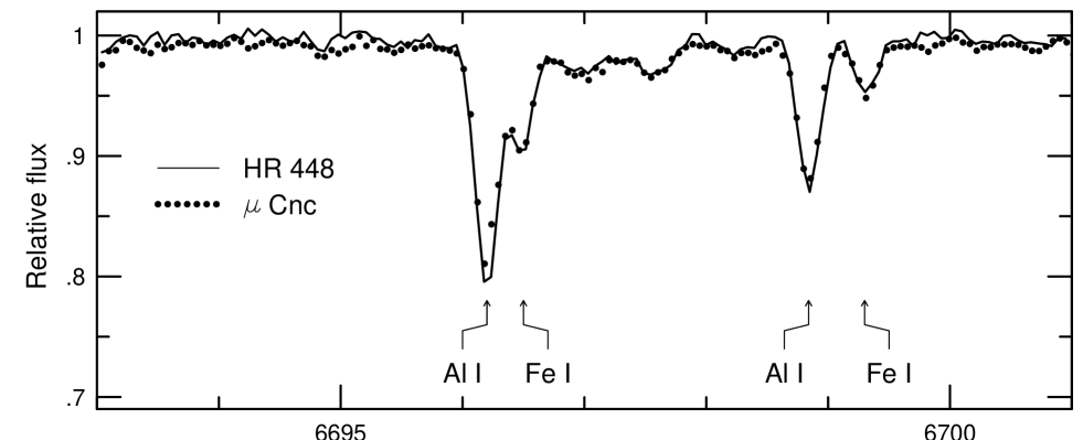
Figure 1 shows the two Al i lines near 6700 Å in a NaMgAl star and a non-NaMgAl star. The two stars have similar effective temperatures and gravities so differences in the strengths of their lines primarily reflect abundance differences. The strengths of the Al i lines relative to the Fe i lines in the two stars are very similar suggesting that any enhancement of Al relative to Fe in the NaMgAl star is small.
The data were processed and wavelength calibrated in a conventional manner with the IRAF package of programs on a SPARC 5 workstation in the Astronomy Department at the University of Texas. Lines suitable for measurement were chosen for clean profiles, as judged by inspection of the solar spectrum at high resolution and signal-to-noise ratio (Kurucz et al. 1984), that provide reliable equivalent widths in all, or most, of the programme stars. Moore et al. (1966) was our primary source of line identification. The equivalent width of each line was measured with the IRAF measurement option most suited to the situation of the line; usually this was the fitting of a single, or multiple, Gaussian profile to the line profile.
Table 2 gives the list of lines measured. The list includes most of the lines used by EAGLNT and many additional ones. In particular our new list contains more Na, Mg and Al lines than theirs; specifically three Na i, four Mg i and seven Al i lines in the new line list compared with two Na i, two Mg i and two Al i lines in theirs. The new line list also has more lines of most other elements and it includes some new elements, notably C and N which are represented by six C i lines and two N i lines.
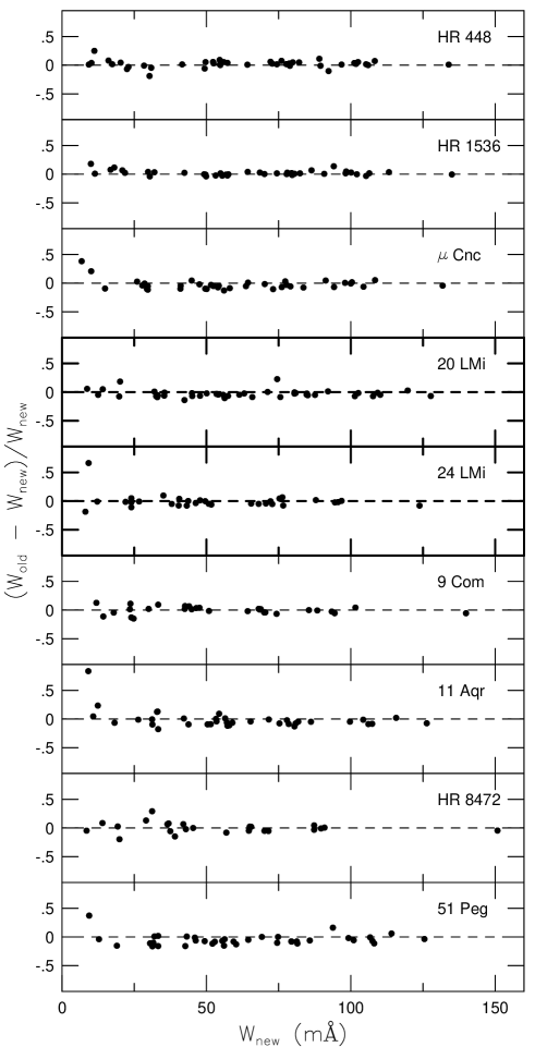
Figure 2 compares our new equivalent widths with those of EAGLNT. The overall agreement is good. In a few cases, however, we note a tendency for the new equivalent widths to be slightly larger than those of EAGLNT; 51 Peg is the most marked case. This can be attributed to the fact that for most of the stars in the programme the resolution (60 000) of the new observations is higher than that (30 000) of EAGLNT’s observations thus leading to a better defined and slightly higher continuum. 222Of the nine stars in our programme seven ( Cnc, 20 LMi, 24 LMi, 9 Com, 11 Aqr, HR 8472, 51 Peg) had been observed from McDonald Observatory at a resolution of 30 000 and two (HR 448, HR 1536) had been observed from ESO at a resolution of 80 000 in EAGLNT’s study. The behaviour of 51 Peg, which as one of the coolest and most metal rich of the stars has one of the most crowded spectra, supports this explanation.
3 Analysis
The LTE abundance analysis was made strictly relative to the Sun and adopts the same procedures, software and model atmospheres as were used by EAGLNT.
3.1 Line data
Basic line data for all the measured transitions were obtained from the VALD atomic line data base (Piskunov et al. 1995) by the “show line” command. Astrophysical oscillator strengths were determined for each line by requiring that the equivalent width derived from the solar model be equal to that measured from the solar flux spectrum as reflected by Iris. The parameters of the solar model are given in Table 1 and the solar chemical abundances were adopted from Grevesse et al. (1996). New quantum mechanical calculations of pressure line-broadening properties by Anstee & O’Mara (1995) and Barklem & O’Mara (1997) were adopted for several lines of s-p, p-s, p-d and d-p transitions in neutral species. There is a small systematic difference between our solar equivalent widths and those measured by EAGLNT. The weakest lines are in the mean about 2% stronger in EAGLNT, and the strongest lines about 2% weaker. This difference/uncertainty (together with the line-broadening mentioned above) is reflected in the values. However, since the programme stars are observed and measured with identical procedures, we neglect the very small differential errors which may be caused by these uncertainties.
| Wλ⊙ | |||||
| Å] | [eV] | s-1 | [mÅ] | ||
| C I | |||||
| 5380.32 | 7.69 | 1.68 | 2.5 | 1.7 106 | 22.3 |
| 6587.62 | 8.54 | 1.14 | 2.5 | 3.9 106 | 14.6 |
| 7111.45 | 8.64 | 1.18 | 2.5 | 1.8 106 | 11.2 |
| 7113.17 | 8.65 | 0.78 | B | 2.5 106 | 22.7 |
| 7115.17 | 8.64 | 0.68 | B | 4.0 106 | 26.8 |
| 7116.96 | 8.16 | 1.30 | 2.5 | 1.4 106 | 18.5 |
| N I | |||||
| 7468.27 | 10.34 | 0.06 | A | 3.1 107 | 4.1 |
| 8629.16 | 10.67 | 0.08 | A | 3.0 107 | 3.4 |
| O I | |||||
| 6158.17 | 10.74 | 0.37 | B | 5.4 107 | 4.2 |
| 7771.95 | 9.14 | 0.36 | A | 4.8 107 | 70.6 |
| 7774.18 | 9.14 | 0.21 | A | 4.7 107 | 60.9 |
| 7775.40 | 9.14 | 0.02 | A | 4.5 107 | 47.9 |
| Na I | |||||
| 4497.68 | 2.10 | 1.59 | 2.0 | 6.4 107 | 39.3 |
| 6154.23 | 2.10 | 1.59 | 2.0 | 6.4 107 | 39.6 |
| 6160.75 | 2.10 | 1.32 | 2.0 | 6.7 107 | 57.7 |
| Mg I | |||||
| 6318.71 | 5.11 | 2.08 | 2.5 | 2.8 105 | 39.8 |
| 6319.24 | 5.11 | 2.28 | 2.5 | 3.0 105 | 27.8 |
| 6965.41 | 5.75 | 1.75 | 2.5 | 3.6 105 | 24.1 |
| 7759.37 | 5.93 | 1.68 | 2.5 | 3.3 105 | 21.0 |
| Al I | |||||
| 6696.03 | 3.14 | 1.59 | 2.5 | 3.0 108 | 38.1 |
| 6698.67 | 3.14 | 1.91 | 2.5 | 3.0 108 | 21.9 |
| 7835.32 | 4.02 | 0.72 | 2.5 | 7.9 107 | 48.1 |
| 7836.13 | 4.02 | 0.57 | 2.5 | 7.9 107 | 61.0 |
| 8772.88 | 4.02 | 0.46 | 2.5 | 8.3 107 | 75.2 |
| 8773.91 | 4.02 | 0.29 | 2.5 | 8.3 107 | 94.4 |
| 8828.87 | 4.09 | 1.89 | 2.5 | 4.2 106 | 4.0 |
| Si I | |||||
| 6125.03 | 5.61 | 1.53 | 1.3 | 1.1 106 | 33.4 |
| 6142.49 | 5.62 | 1.47 | 1.3 | 8.8 105 | 36.5 |
| 6145.02 | 5.61 | 1.42 | 1.3 | 9.8 105 | 39.9 |
| 6155.14 | 5.62 | 0.75 | 1.3 | 3.6 106 | 88.7 |
| 6848.57 | 5.86 | 1.65 | 1.3 | 1.1 106 | 18.3 |
| 7455.39 | 5.96 | 2.01 | 1.3 | 4.0 105 | 7.5 |
| 7800.00 | 6.18 | 0.73 | 1.3 | 3.3 106 | 55.7 |
| S I | |||||
| 6046.02 | 7.87 | 0.41 | 2.5 | 1.0 107 | 17.3 |
| 6743.58 | 7.87 | 0.64 | 2.5 | 1.1 107 | 10.3 |
| 7686.13 | 7.87 | 1.15 | 2.5 | 1.7 106 | 3.4 |
| K I | |||||
| 5801.75 | 1.62 | 1.51 | 2.5 | 3.1 106 | 2.0 |
| 7698.98 | 0.00 | 0.01 | A | 5.8 107 | 159.5 |
| Wλ⊙ | |||||
| Å] | [eV] | s-1 | [mÅ] | ||
| Ca I | |||||
| 5867.57 | 2.93 | 1.64 | 1.8 | 2.6 108 | 25.3 |
| 6166.44 | 2.52 | 1.22 | B | 1.9 107 | 71.7 |
| 6169.04 | 2.52 | 0.88 | B | 2.0 107 | 96.0 |
| 6455.61 | 2.52 | 1.43 | A | 4.6 107 | 58.6 |
| 6464.68 | 2.52 | 2.41 | A | 4.6 107 | 12.6 |
| 6572.80 | 0.00 | 4.33 | A | 2.6 107 | 33.6 |
| Sc I | |||||
| 5520.51 | 1.87 | 0.62 | A | 9.3 107 | 9.0 |
| Sc II | |||||
| 5318.36 | 1.36 | 1.81 | 2.5 | 1.4 108 | 13.5 |
| 6245.62 | 1.51 | 1.10 | 2.5 | 4.3 108 | 36.7 |
| 6604.60 | 1.36 | 1.25 | 2.5 | 1.5 108 | 37.0 |
| Ti I | |||||
| 5113.45 | 1.44 | 0.91 | A | 2.2 107 | 27.5 |
| 5219.71 | 0.02 | 2.29 | A | 6.7 106 | 28.7 |
| 5426.26 | 0.02 | 3.11 | A | 1.7 106 | 6.2 |
| 5766.33 | 3.29 | 0.26 | B | 1.4 108 | 9.4 |
| 5866.46 | 1.07 | 0.88 | A | 6.4 107 | 48.7 |
| 6091.18 | 2.27 | 0.47 | A | 8.5 107 | 15.9 |
| 6126.22 | 1.07 | 1.44 | A | 9.9 106 | 22.8 |
| 6258.11 | 1.44 | 0.47 | A | 1.7 108 | 52.2 |
| V I | |||||
| 5727.06 | 1.08 | 0.03 | A | 7.1 107 | 39.4 |
| 6039.74 | 1.06 | 0.73 | A | 4.0 107 | 13.3 |
| 6090.22 | 1.08 | 0.15 | A | 4.0 107 | 34.2 |
| 6111.65 | 1.04 | 0.80 | A | 3.9 107 | 12.1 |
| 6216.36 | 0.28 | 0.87 | A | 3.1 106 | 38.4 |
| 6224.51 | 0.29 | 1.91 | A | 1.2 106 | 5.7 |
| 6251.83 | 0.28 | 1.42 | A | 3.1 106 | 15.8 |
| Cr I | |||||
| 6330.10 | 0.94 | 2.94 | A | 2.4 107 | 27.1 |
| Cr II | |||||
| 5305.87 | 3.83 | 2.06 | 2.5 | 2.6 108 | 26.6 |
| Fe I | |||||
| 5067.16 | 4.22 | 0.96 | B | 2.1 108 | 73.5 |
| 5090.78 | 4.26 | 0.61 | B | 2.1 108 | 96.5 |
| 5109.66 | 4.30 | 0.82 | B | 2.1 108 | 79.4 |
| 5141.75 | 2.42 | 2.20 | A | 1.5 108 | 89.6 |
| 5358.12 | 3.30 | 3.20 | A | 2.0 108 | 10.3 |
| 5809.22 | 3.88 | 1.70 | A | 5.1 107 | 50.6 |
| 5849.69 | 3.69 | 2.98 | A | 5.5 107 | 7.8 |
| 5852.23 | 4.55 | 1.23 | B | 1.9 108 | 41.2 |
| 5855.09 | 4.61 | 1.57 | B | 1.9 108 | 22.4 |
| 5856.10 | 4.29 | 1.60 | 1.4 | 8.6 107 | 33.4 |
| 5858.79 | 4.22 | 2.20 | B | 2.7 108 | 13.8 |
| 5859.60 | 4.55 | 0.71 | B | 1.9 108 | 72.8 |
| 5861.11 | 4.28 | 2.36 | B | 2.1 108 | 8.9 |
| 5862.37 | 4.55 | 0.49 | B | 1.9 108 | 88.4 |
| 6151.62 | 2.18 | 3.30 | A | 1.6 108 | 50.9 |
| 6157.73 | 4.08 | 1.22 | 1.4 | 5.0 107 | 63.4 |
| 6159.38 | 4.61 | 1.88 | B | 1.9 108 | 12.6 |
| 6165.36 | 4.14 | 1.50 | 1.4 | 8.8 107 | 46.3 |
| 6173.34 | 2.22 | 2.88 | A | 1.7 108 | 69.7 |
| 6200.32 | 2.61 | 2.39 | A | 1.0 108 | 75.3 |
| 6436.41 | 4.19 | 2.39 | 1.4 | 3.0 107 | 10.2 |
| Wλ⊙ | |||||
| Å] | [eV] | s-1 | [mÅ] | ||
| Fe I cont. | |||||
| 6591.33 | 4.59 | 1.99 | 1.4 | 1.4 108 | 10.8 |
| 6608.04 | 2.28 | 3.95 | A | 1.7 108 | 18.7 |
| 6699.14 | 4.59 | 2.12 | 1.4 | 1.4 108 | 8.4 |
| 6713.75 | 4.80 | 1.44 | B | 2.4 108 | 21.5 |
| 6725.36 | 4.10 | 2.21 | A | 2.1 108 | 17.9 |
| 6732.07 | 4.58 | 2.21 | 1.4 | 6.0 107 | 7.1 |
| 6733.15 | 4.64 | 1.43 | 1.4 | 2.3 108 | 27.7 |
| 6857.25 | 4.08 | 2.07 | 1.4 | 2.5 107 | 23.5 |
| 7751.12 | 4.99 | 0.80 | B | 6.4 108 | 46.5 |
| 7802.51 | 5.09 | 1.36 | B | 6.3 108 | 16.1 |
| 7844.57 | 4.84 | 1.71 | 1.4 | 2.3 108 | 12.8 |
| 8747.44 | 3.02 | 3.35 | A | 8.0 107 | 18.1 |
| 8757.20 | 2.84 | 2.01 | A | 7.7 106 | 97.4 |
| Fe II | |||||
| 5100.66 | 2.81 | 4.15 | 2.5 | 3.4 108 | 22.1 |
| 5256.93 | 2.89 | 4.08 | 2.5 | 3.4 108 | 22.1 |
| 5425.26 | 3.20 | 3.31 | 2.5 | 3.0 108 | 41.8 |
| 5427.80 | 6.72 | 1.53 | 2.5 | 3.5 108 | 4.4 |
| 6149.25 | 3.89 | 2.78 | 2.5 | 3.4 108 | 37.0 |
| 6247.56 | 3.89 | 2.41 | 2.5 | 3.4 108 | 54.4 |
| 6369.46 | 2.89 | 4.16 | 2.5 | 2.9 108 | 19.9 |
| 6383.72 | 5.55 | 2.11 | 2.5 | 4.1 108 | 9.8 |
| 6432.68 | 2.89 | 3.64 | 2.5 | 2.9 108 | 41.6 |
| 6456.39 | 3.90 | 2.20 | 2.5 | 3.4 108 | 64.7 |
| 7479.70 | 3.89 | 3.67 | 2.5 | 3.1 108 | 9.3 |
| 7515.84 | 3.90 | 3.50 | 2.5 | 4.1 108 | 12.6 |
| 7841.37 | 3.90 | 4.04 | 2.5 | 3.0 108 | 4.3 |
| Ni I | |||||
| 5082.35 | 3.66 | 0.59 | B | 1.8 108 | 67.9 |
| 5084.11 | 3.68 | 0.13 | B | 1.3 108 | 94.8 |
| 5088.54 | 3.85 | 1.08 | B | 1.6 108 | 33.5 |
| 5088.96 | 3.68 | 1.30 | B | 1.3 108 | 30.4 |
| 5094.42 | 3.83 | 1.14 | B | 1.2 108 | 31.3 |
| 5102.97 | 1.68 | 2.77 | A | 1.3 108 | 51.3 |
| 5115.40 | 3.83 | 0.35 | 2.5 | 7.3 107 | 78.6 |
| 5847.01 | 1.68 | 3.44 | A | 7.4 107 | 23.3 |
| 6111.08 | 4.09 | 0.83 | B | 1.5 108 | 36.1 |
| 6130.14 | 4.27 | 0.97 | B | 2.8 108 | 22.4 |
| 6133.98 | 4.09 | 1.80 | B | 1.4 108 | 6.1 |
| 6175.37 | 4.09 | 0.55 | B | 2.3 108 | 50.9 |
| 6176.82 | 4.09 | 0.29 | B | 1.5 108 | 65.4 |
| 6177.25 | 1.83 | 3.54 | 2.5 | 4.3 107 | 15.3 |
| 6204.61 | 4.09 | 1.14 | A | 1.8 108 | 23.2 |
| 6378.26 | 4.15 | 0.85 | B | 2.1 108 | 32.8 |
| 6850.44 | 3.68 | 1.99 | A | 9.9 107 | 10.0 |
| 7748.89 | 3.71 | 0.39 | A | 9.5 107 | 90.5 |
| 7797.59 | 3.90 | 0.38 | A | 1.0 108 | 80.6 |
| 7826.77 | 3.70 | 1.87 | A | 8.0 107 | 13.1 |
| Y II | |||||
| 5087.43 | 1.08 | 0.36 | 2.5 | 1.3 107 | 48.3 |
| 5200.42 | 0.99 | 0.65 | 2.5 | 1.1 107 | 39.9 |
| 5402.78 | 1.84 | 0.58 | 2.5 | 8.6 106 | 12.8 |
| Zr I | |||||
| 6127.48 | 0.15 | 0.92 | A | 2.4 106 | 3.8 |
| 6134.57 | 0.00 | 1.20 | A | 2.2 106 | 2.8 |
| Wλ⊙ | |||||
| Å] | [eV] | s-1 | [mÅ] | ||
| Zr II | |||||
| 5112.28 | 1.66 | 0.78 | 2.5 | 1.1 107 | 9.7 |
| Ba II | |||||
| 5853.69 | 0.60 | 0.99 | 3.0 | 1.6 108 | 64.2 |
| 6141.73 | 0.70 | 0.08 | 3.0 | 1.6 108 | 119.5 |
| 6496.91 | 0.60 | 0.40 | 3.0 | 1.3 108 | 102.7 |
| Eu II | |||||
| 6645.13 | 1.38 | 0.24 | 2.5 | 2.4 107 | 5.3 |
A few lines were excluded from the analysis after a first abundance analysis of all stars, since they give abundances that deviate strongly, often as a function of effective temperature, from those of other lines of the same species: Sc i 6239.36, Ti i 5299.98, V i 6150.15, Fe i 5127.37, Ni i 5099.94 and 7788.15 and Y i 6687.51 Å. For some of these, asymmetries could be traced in the spectra, while for others we suspect undetected blends or line misidentifications. For the 7788.15 Å Ni i line a laboratory oscillator strength is quoted in the VALD data base which is 0.5 dex lower than our solar value, which means that most of the observed line absorption in the Sun may be caused by another transition. Therefore, these lines were not used. Also the Sc ii 5318.36 Å line was found to be asymmetric in the two hottest stars and was not used for 9 Com and HR 8472.
The solar equivalent widths and adopted line data are given in Table 2.
3.2 Model atmosphere parameters
Initially, the model parameters , and [Fe/H] were adopted from EAGLNT, as well as microturbulence parameters computed from their Eq. (9). The larger set of observed spectral lines in this project enables the application of better spectroscopic statistical checks on the individual stellar effective temperatures, microturbulence parameters and surface gravities. The initial values were then iteratively modified as described below. Since, for metal-rich stars, the temperature structures of the model atmospheres are rather sensitive to the overall metallicity, the model metallicities were kept consistent with the [Fe/H] values obtained in the analysis.
-
1.
Erroneous effective temperatures show up (assuming) LTE as systematic dependences of derived line-by-line abundances as a function of line excitation energy. To investigate such effects, the abundances of Fe i and Ni i lines with reduced equivalent widths less than (to reduce the influence of possible uncertainties in the line broadening) were plotted versus the excitation energy of the lower level. To avoid systematic errors due to random equivalent width measurement errors, theoretical equivalent widths, , as suggested by Magain (1984) were used for this check. The effective temperature of each star was then modified to minimise these slopes.
-
2.
Similarly, inconsistent microturbulences should result in abundances which vary as a function of line strength for different lines of a species. For this test the Fe i and Ni i lines with excitation energies eV (to minimise possible effects of errors in the excitation balances) were plotted against . The microturbulence parameter of each star was then modified to minimise these slopes.
-
3.
The surface gravities were then determined by synthesis of the spectral region near the strong Ca i 6162.17 Å line, the wings of which are sensitive to the gas pressure and therefore to surface gravity (cf. e.g. Edvardsson 1988).
-
4.
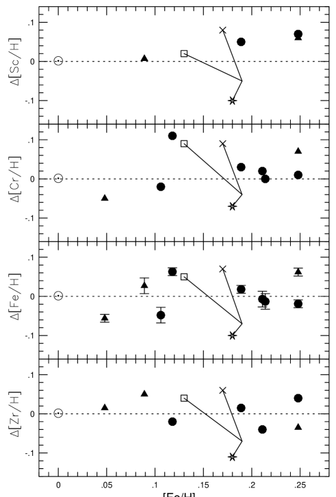
As a fourth consistency check, the ionization balances, which in the LTE assumption are sensitive to the effective temperatures and surface gravities via the Saha equation, were studied for four elements which are represented by both neutral and singly ionised lines in the investigation: Sc, Cr, Fe and Zr. While there are many Fe i and Fe ii lines measured, the numbers of measured lines for the other species are few: only one line for Sc i, Cr i, Cr ii and Zr ii, and at most three lines for Sc ii and Zr i. Nevertheless, all the four elements show very similar sensitivities to the stellar parameters and give consistent indications of the surface gravity for a reasonable choice of effective temperature. This is demonstrated in Fig. 3.
These four checks were then performed while the atmospheric parameters were iterated until good consistency was obtained for each individual star. The finally adopted atmospheric parameters are given in Table 1.
It is now of interest to investigate how these parameters deviate from the values in EAGLNT, which were determined from Strömgren photometry. The new effective temperatures are K with a dispersionof K hotter, which is actually somewhat less than what was found in an excitation-equilibrium test in Sect. 4.3.4 of EAGLNT. The new surface gravities are dex with a dispersion of dex higher than those of EAGLNT, which is within the total expected uncertainty given in their Sect. 4.2.1. Our [Fe/H] values differ from the photometric metallicities of EAGLNT by dex (dispersion), and finally the microturbulence parameters are km s-1 higher than Eq. 9 of EAGLNT would give for the new values of and . No systematic dependence of these differences on the atmospheric parameters themselves can be seen.
3.3 Errors in the resulting abundances
An extensive discussion of error sources (e.g., NLTE-effects and oversimplification of the model atmospheres) in an analysis which is very similar to the present one was given by EAGLNT, and will not be repeated here. We note, however, that we now have a much larger sample of spectral lines, and that the equivalent widths are more accurate. Furthermore, the present sample of stars spans a small range in metallicity and a range of only 10% in effective temperature, so much of the actual errors cancel in an analysis relative to the Sun.
Figure 3 shows the remaining small differences between the absolute abundances of an element as derived from two different states of ionization. Only for iron are there several lines measured from both the neutral and the ionized species, and the error bars show the formal errors of the mean abundances (calculated from the internal scatter among Fe i and Fe ii lines, respectively) added in quadrature.
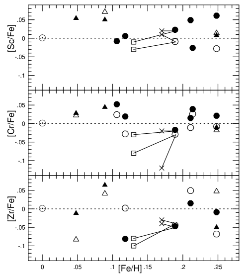
Also the abundance ratios relative to Fe, [X/Fe], for these elements are very similar if data from neutral and ionized lines are used, as can be seen in Fig. 4. This confirms the good quality of the equivalent width measurements.
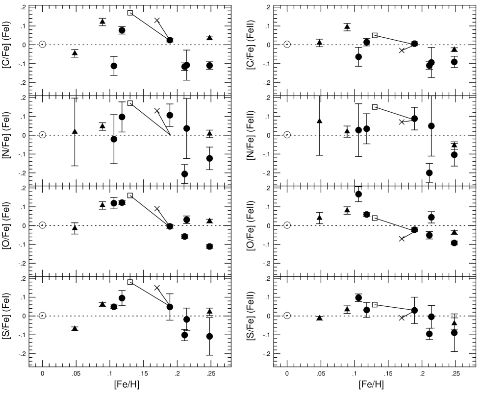
For C, N, O and S, the (high-excitation) lines used are of the neutral atom which is the dominant species due to their high ionization energies. When abundance ratios to the iron atom are plotted one finds that the ratios decrease systematically with increasing metallicity. If the ratios are instead taken with respect to the majority species Fe ii the amounts of scatter around the trends diminish appreciably. This is shown in Fig. 5. The sensitivity of the abundance ratios to effective temperature and surface gravity are clearly different, which, together with the smaller scatter, suggests that the ratios relative to Fe ii are the more accurate.
4 Results
The resulting abundances for the nine stars are given in Table 3, and the line-by-line measured equivalent widths and abundances are given in Table 4 (available in electronic form).
| Species | HR 448 | HR 1536 | HR 3176 | HR 3951 | HR 4027 | HR 4688 | HR 8041 | HR 8472 | HR 8729 | |
|---|---|---|---|---|---|---|---|---|---|---|
| Cnc | 20 LMi | 24 LMi | 9 Com | 11 Aqr | 51 Peg | |||||
| Fe i | 22–34 | 0.12.01 | 0.21.01 | 0.09.01 | 0.25.00 | 0.05.00 | 0.21.01 | 0.25.00 | 0.11.01 | 0.19.00 |
| C i | 3–6 | 0.20.02 | 0.09.02 | 0.21.02 | 0.14.02 | 0.00.02 | 0.11.08 | 0.28.01 | -0.01.05 | 0.21.01 |
| N i | 2 | 0.22.08 | 0.00.05 | 0.14.02 | 0.12.06 | 0.06.18 | 0.25.16 | 0.25.02 | 0.09.13 | 0.30.06 |
| O i | 3–4 | 0.24.01 | 0.15.00 | 0.20.01 | 0.14.00 | 0.03.03 | 0.25.02 | 0.27.01 | 0.22.03 | 0.19.00 |
| Na i | 2–3 | 0.22.01 | 0.23.01 | 0.20.01 | 0.27.01 | 0.06.00 | 0.30.01 | 0.35.01 | 0.17.02 | 0.26.01 |
| Mg i | 1–4 | 0.23.06 | 0.21.05 | 0.14.05 | 0.23.05 | 0.06.06 | 0.07 | 0.23.05 | 0.08.16 | 0.18.10 |
| Al i | 4–7 | 0.19.01 | 0.26.01 | 0.19.01 | 0.27.01 | 0.10.01 | 0.26.02 | 0.27.01 | 0.16.01 | 0.21.01 |
| Si i | 5–7 | 0.20.01 | 0.25.01 | 0.15.01 | 0.26.01 | 0.07.01 | 0.25.01 | 0.30.01 | 0.17.02 | 0.24.01 |
| S i | 2–3 | 0.21.03 | 0.11.03 | 0.15.01 | 0.14.10 | -0.02.01 | 0.20.05 | 0.27.02 | 0.16.01 | 0.24.07 |
| K i | 0–2 | 0.16 | 0.21 | 0.13 | 0.16.00 | 0.16.04 | — | 0.18.03 | 0.27 | 0.15.01 |
| Ca i | 3–6 | 0.10.01 | 0.23.01 | 0.07.01 | 0.25.01 | 0.06.01 | 0.20.01 | 0.20.01 | 0.10.04 | 0.16.00 |
| Sc i | 0–1 | — | — | 0.16 | 0.22 | — | — | 0.26 | — | 0.18 |
| Sc ii | 2–3 | 0.19.02 | 0.25.02 | 0.17.04 | 0.29.02 | 0.05.03 | 0.17.02 | 0.32.02 | 0.05.03 | 0.23.01 |
| Ti i | 4–8 | 0.11.01 | 0.25.01 | 0.11.02 | 0.28.01 | 0.09.02 | 0.24.03 | 0.23.01 | 0.10.03 | 0.19.01 |
| V i | 4–7 | 0.11.01 | 0.26.01 | 0.11.02 | 0.31.01 | 0.07.02 | 0.21.02 | 0.27.01 | 0.08.02 | 0.22.01 |
| Cr i | 0–1 | 0.09 | 0.20 | — | 0.24 | 0.07 | 0.24 | 0.23 | 0.13 | 0.16 |
| Cr ii | 1 | 0.20 | 0.22 | 0.16 | 0.25 | 0.02 | 0.24 | 0.30 | 0.11 | 0.19 |
| Fe ii | 8–13 | 0.18.01 | 0.20.02 | 0.12.01 | 0.23.01 | -0.01.01 | 0.20.02 | 0.31.01 | 0.06.02 | 0.21.01 |
| Ni i | 11–20 | 0.15.01 | 0.25.01 | 0.13.01 | 0.27.01 | 0.04.00 | 0.23.01 | 0.30.01 | 0.11.02 | 0.23.00 |
| Y ii | 3–3 | 0.08.03 | 0.21.01 | 0.06.03 | 0.24.01 | -0.07.02 | 0.20.02 | 0.22.01 | 0.09.04 | 0.15.01 |
| Zr i | 0–2 | 0.12.10 | 0.26.11 | 0.13 | 0.18.00 | -0.04.06 | — | 0.30.05 | — | 0.15.08 |
| Zr ii | 0–1 | 0.10 | 0.22 | 0.18 | 0.22 | -0.02 | — | 0.26 | — | 0.16 |
| Ba ii | 2–3 | 0.04.02 | 0.17.01 | -0.03.01 | 0.21.01 | -0.03.01 | 0.12.01 | 0.16.01 | 0.04.04 | 0.12.01 |
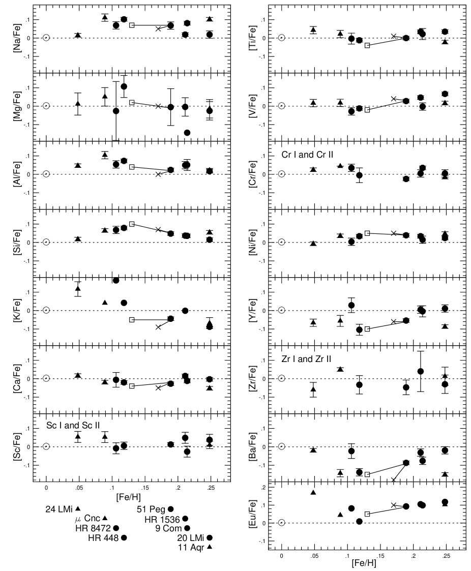
Most of the elements under investigation have ionization energies and partition functions such that the majority of the atoms are in the singly ionized state in the line-forming layers of these solar-type stars. When we display abundance ratios between different elements, we will prefer to display ratios using abundances derived from lines of the same ionization state in the nominator and the denominator. This procedure minimises the effects of remaining uncertainties in the model atmospheres, in the assumptions made in the analysis and in the stellar fundamental parameters. The exceptions to this rule are C, N, O and S as discussed above.
Fig. 6 displays our abundance results, where abundance ratios are plotted as a function of [Fe/H] derived from Fe I lines. In the figure we have also indicated the sensitivity of the abundance ratios to uncertainties in the effective temperatures and surface gravities. The results for C, N, O and S were already shown in Fig. 5.
In spite of the small number of stars the high accuracy in the analysis makes it worthwhile to compare the results with abundance trends found in other analyses. We postpone, however, this discussion to Feltzing & Gustafsson (1997).
Inspection of Fig. 6 shows there are no significant differences between the [Na/Fe], [Mg/Fe] and [Al/Fe] ratios of the NaMgAl stars and the non-NaMgAl stars. The six NaMgAl stars have average abundances [Na/Fe] (standard deviation of the mean), [Mg/Fe] and [Al/Fe] , while the three stars not identified as NaMgAl stars have [Na/Fe] , [Mg/Fe] and [Al/Fe] . (These results use abundances, including those of Fe, from neutral lines.) A larger number of stars not identified as NaMgAl stars may be found in EAGLNT; for the 18 non-NaMgAl stars of EAGLNT with [Fe/H] and abundances derived from EAGLNT’s high resolution (80 000) ESO observations, we find average abundances of [Na/Fe] , [Mg/Fe] and [Al/Fe] . Evidently, the NaMgAl stars have no significant enhancements of Na, Mg or Al and any possible enrichment of these elements is limited to dex, or less.
In view of our failure to confirm the Na, Mg and Al overabundances of the NaMgAl stars claimed by EAGLNT, we now briefly review the sources of difference between our new abundances and those of EAGLNT. Five primary potential sources of differences between the abundances of the two investigations may be listed:
-
1.
Use of additional/different lines
-
2.
Different equivalent widths, stellar and solar
-
3.
Different model parameters
-
4.
Different types of models
-
5.
Different values
The two investigations use the same types of model atmospheres - line blanketed, flux constant, LTE models calculated from a development of the programmes of Gustafsson et al. (1975) - and both use astrophysical oscillator strengths derived from the lines’ equivalent widths in the solar flux spectrum. Item four is, thus, not a factor in the comparison, while item five is subsumed under item two. The causes of the differences between the two investigations are, therefore, to be found in items one, two and three. (A comparison of [Fe/H] abundances with EAGLNT shows that the present [Fe/H] values are significantly higher, by 0.08 dex at a mean. This is for most stars due to the systematically somewhat higher s and s and lower microturbulence parameters of the present analysis, and is within the range of systemic errors ascribed by EAGLNT to their [Fe/H] values. For 51 Peg the larger equivalent widths found here (Fig. 2) are the main cause.) We now do a budget on a line-by-line basis for Na, Mg and Al of the sources of the abundance differences for one of the stars (51 Peg) which EAGLNT identified as a NaMgAl star.
In Table 5 we compare our new equivalent widths and EAGLNT’s for 51 Peg and the Sun for the Na i and Al i lines in common to our investigation and theirs; the two investigations do not have any Mg lines in common. A comparison of our new model atmosphere parameters for 51 Peg (Table 1) and EAGLNT’s reveals modest revisions, namely an increase of 20 K in the effective temperature, an increase of 0.17 in , a decrease of 0.22 km s-1 in microturbulence and an increase of 0.11 dex in [M/H]. The separate effects on the Na and Al abundances of the equivalent width and changes and these revisions of the model parameters are also shown in Table 5. For the Na i and Al i lines in common to the two analyses the new analysis gives [Na/H] = +0.25 and [Al/H] = +0.21, while for the same lines EAGLNT found [Na/H] = +0.22 and [Al/H] = +0.28. The abundance differences, for the same lines, between the new analysis and EAGLNT’s, therefore, are [Na/H] = +0.03 and [Al/H] = –0.07, which for both elements differ by only 0.01 dex from the total of the separate effects listed in Table 5. For the lines in common to the two investigations, therefore, the changes in the Na and Al abundances are almost entirely due to changes of the stellar equivalent widths, the and the model atmosphere parameters.
| Line | [Å] | Wλ [mÅ] new | Wλ [mÅ] EAGLNT | [X/H] (new – EAGLNT) | ||||||||||
|---|---|---|---|---|---|---|---|---|---|---|---|---|---|---|
| 51 Peg | Sun | 51 Peg | Sun | Wλ | [M/H] | Total | ||||||||
| Na i | 6154.23 | 56.3 | 39.6 | 54.1 | 38.2 | +0.03 | –0.02 | +0.01 | –0.01 | +0.02 | +0.01 | +0.04 | ||
| Na i | 6160.75 | 74.8 | 57.7 | 74.9 | 58.6 | 0.00 | +0.01 | +0.01 | –0.01 | +0.02 | +0.01 | +0.04 | ||
| Average | +0.04 | |||||||||||||
| Al ia | 8772.88 | 93.8 | 75.2 | 109.0 | 80.4 | –0.15 | +0.05 | +0.01 | –0.04 | +0.02 | +0.01 | –0.10 | ||
| Al i | 8773.91 | 114.1 | 94.4 | 121.0 | 98.1 | –0.06 | +0.04 | +0.01 | –0.04 | +0.02 | +0.01 | –0.02 | ||
| Average | –0.06 | |||||||||||||
| aThe new equivalent width of this line in 51 Peg is 15.2 mÅ smaller than EAGLNT’s measurement. This poor agreement is caused by a nearby weaker unidentified line at 8772.54 Å, which at the 60 000 resolution of the new observations is partially resolved from the Al i line and is excluded from the new equivalent width, but at the lower 30 000 resolution used by EAGLNT for 51 Peg was blended with the Al i line and was included in their equivalent width. In the Sun this nearby line is excluded from both the new and EAGLNT equivalent widths | ||||||||||||||
For all three Na i lines used in the new analysis the average [Na/H] is (standard deviation of the mean) which is very similar to the new analysis’s value of for the two lines in common with EAGLNT’s analysis, while for all seven Al i lines used in the new analysis the [Al/H] is which is the same as the new analysis’s value of for the two lines in common with EAGLNT’s analysis. The additional Na i and Al i lines of the new analysis thus serve to confirm the abundances derived from the Na i and Al i lines in common with EAGLNT’s analysis.
EAGLNT’s Na, Mg and Al abundances were based on only two lines for each element and one of the Mg lines (Mg i 8712.69 Å) and one of the Al lines (Al i 8772.87 Å) are not of top quality 333The 8712.69 Å Mg i line is close to a stronger Fe i line at 8713.21 Å; it is not used here. The 8772.87 Å Al i line is partially blended with a much weaker, but not insignificant, unidentified line at 8772.54 Å. This Al i line, which at the resolution (60 000) of the present investigation can be reliably measured in sharp-lined stars, is used here (see Table 2). so their abundances for these elements were less accurate than for elements with good spectral representation such as Fe or Ni. Overinterpretation of their results for Na, Mg and Al, thus, tempted them to see overabundances of these three elements where none actually existed. The preponderance of NaMgAl stars they observed at McDonald Observatory compared with ESO is consistent with such an explanation. The 189 stars in EAGLNT were made up of 102 northern stars observed from McDonald Observatory at a resolution of 30 000, 71 southern stars observed from ESO at resolutions of 60 000 and 80 000 and 16 stars observed from both observatories. Of the eight suggested NaMgAl stars six were observed from McDonald Observatory and only two were observed from ESO. The disproportionately large number of “detections” among their McDonald stars can be attributed to the larger observational scatter of the abundances, derived from the lower resolution McDonald spectra.
Inspection of Fig. 5 and 6 shows nothing unusual about 51 Peg compared to the other stars in these plots and so, although 51 Peg is metal rich, we find no sign of its composition being distinctive compared to other metal rich stars of similar spectral type.
Finally we briefly discuss our new determination of 51 Peg’s metallicity. Our result, [Fe/H] , is higher than the earlier result of EAGLNT who found [Fe/H] and is almost identical to the results of Valenti (1994) and Gonzalez (1997) who found [Fe/H] of and , respectively. Both Valenti’s and Gonzalez’s studies are also based on high-resolution spectroscopic observations. Most of the increase of our [Fe/H] compared with EAGLNT’s is a consequence of our new equivalent widths, with smaller increases being caused by the higher effective temperature ( K) and lower microturbulence () used in the new analysis. Valenti and Gonzalez both use very similar model atmosphere parameters for 51 Peg to ours; Valenti adopts K, and km s-1 and Gonzalez adopts K, and km s-1, while we adopt (Table 1) K, and km s-1.
5 Conclusions
Our new study does not confirm the Na, Mg and Al overabundances EAGLNT claimed to find. With the aid of new spectra, that for most stars have higher spectral resolution and include more Na, Mg and Al lines than EAGLNT were able to use, we find that the Na, Mg and Al abundances of the NaMgAl stars are the same to within dex as those of non-NaMgAl stars of similar temperature, gravity and metallicity. The group thus appears to be illusory and so should be deleted from the inventory of chemically peculiar stars.
The demise of the NaMgAl group of stars removes the basis for EAGLNT’s speculation that these stars, and 51 Peg in particular, may have stellar remnant companions. The identification of 51 Peg’s companion as a planet, thus, becomes more secure. We note, however, Gray’s (1997) recent claim that the regular 4.23 d radial velocity variation of 51 Peg is of pulsational origin, rather than a result of reflex orbital motion. Clearly this question must be settled before one can be sure that 51 Peg really has a planetary companion.
Acknowledgements.
We thank Al Wootten for pointing out that 51 Peg was one of the stars in EAGLNT’s survey, Brian Marsden for providing an ephemeris for Iris and Paul Barklem and Jim O’Mara for calculating and sending us line broadening data before publication. DLL and JT acknowledge support from the US National Science Foundation (grant AST 93-15124) and the Robert A. Welch Foundation. BE and BG acknowledge support from the Swedish Natural Sciences Research Council.References
- [1] Anstee S.D., O’Mara B.J., 1995, MNRAS 276, 859
- [2] Barklem P.S., O’Mara B.J., 1997, MNRAS, submitted
- [3] Butler R.P., Marcy, G.W., Williams E., Hauser H., Shirts P., 1997, ApJ 474, L115
- [4] Edvardsson B., 1988, A&A 190, 148
- [5] Edvardsson B., Andersen J., Gustafsson B., Lambert D.L., Nissen P.E., Tomkin J., 1993, A&A 275, 101 (EAGLNT)
- [6] Feltzing S., Gustafsson B., 1997, A&A, submitted
- [7] Gonzalez G., 1997, PASP, submitted
- [8] Gray D.F., 1997, Nature 385, 795
- [9] Grevesse N., Noels A., Sauval A.J., 1996, in ASP Conf. Ser. 99, eds. S.S. Holt, G. Sonneborn, p. 117
- [10] Gustafsson B., Bell R.A., Eriksson K., Nordlund Å, 1975, A&A 42, 407
- [11] Kurucz R.L., Furenlid I., Brault J., Testerman L., 1984, Solar Flux Atlas from 296 to 1300 nm, National Solar Observatory, Sunspot, New Mexico
- [12] Magain P., 1984, A&A 134, 189
- [13] Marcy G.W., Butler R.P., Williams E., et al., 1997, ApJ, submitted
- [14] Mayor M., Queloz D., 1995, Nature 378, 355
- [15] Moore C.E., Minnaert M.G.J., Houtgast J., 1966, The Solar Spectrum 2935 Å to 8770 Å, National Bureau of Standards, Monograph 61
- [16] Piskunov N.P., Kupka F., Ryabchikova T.A., Weiss W.W., Jeffery C.S., 1995, A&AS 112, 525
- [17] Tull R.G., MacQueen P.J., Sneden C., Lambert D.L., 1995, PASP 107, 251
- [18] Valenti J.A., 1994, PhD thesis, Univ. of Colorado