Fluctuations in finite $N$ equilibrium stellar systems

Abstract

Gravitational amplification of Poisson noise in stellar systems is important on large scales. For example, it increases the dipole noise power by roughly a factor of six and the quadrupole noise by 50% for a King model profile. The dipole noise is amplified by a factor of fifteen for the core-free Hernquist model. The predictions are computed using the dressed-particle formalism of Rostoker & Rosenbluth (1960) and are demonstrated by n-body simulation.

This result implies that a collisionless n-body simulation is impossible; The fluctuation noise which causes relaxation is an intrinic part of self gravity. In other words, eliminating two-body relaxation does not eliminate relaxation altogether.

Applied to dark matter halos of disk galaxies, particle numbers of at least $10^{6}$ will be necessary to suppress this noise at a level that does not dominate or significantly affect the disk response. Conversely, halos are most likely far from phase-mixed equilibrium and the resulting noise spectrum may seed or excite observed structure such as warps, spiral arms and bars. For example, discreteness noise in the halo, similar to that due to a population of $10^{6}M_{\odot}$ black holes can produce observable warping and possibly excite or seed other disk structure.

1 Introduction

Stellar systems are finite number systems by nature. Because the characteristic relaxation time is so long in many cases of astronomical interest, the continuum limit is a good approximation and the collisionless Boltzmann equation (CBE) governs the evolution. Because the CBE is difficult to solve in any generality, many researchers have turned to n-body simulation as a primary source of insight. For a modest number of particles, however, the naive n-body problem is not a simulation of the CBE but of the collisional Boltzmann equation. Enormous effort has been applied to manipulating the interparticle force to reduce the intrinsic relaxation to produce a near-collisionless solution. The most commonly used technique smoothes the particle over a finite size region leading to the softened the point mass potential: $G\mu/r\rightarrow G\mu/\sqrt{r^{2}+a^{2}}$. As long as the smoothing size is not larger than the mean interparticle spacing, intuitively, there should be no significant change in the results.

Unfortunately, two-body interactions are only part of the story. Poisson fluctuations excite structure at all scales in the system. Many simulations are optimized to resolve large-scale features but the relaxation is enhanced by large-scale collective excitations on these same scales (Weinberg 1993). One can think of this excitation as the projection Poisson noise on the modal spectrum of the stellar system. This is the same modal spectrum responsible for producing a response by a perturber of interest, such as a galaxy reacting to orbiting or passing companion. Therefore, a collisionless solution is physically impossible without irrevocably changing the dynamics of the system under study. In other words, one suppresses the global part of the relaxation at the risk of throwing out the physics responsible for the evolution one is studying. There is no other recourse but large numbers of particles.

For example, this work was motivated by n-body experiments with a thin disk in a live halo. The observed fluctuations vertical in force at the disk plane were larger than predicted for Poisson fluctuations for n-body simulations of halos with $10^{5}$ particles using the SCF scheme (e.g. Clutton-Brock 1972, 1973, Hernquist & Ostriker 1992). However, real galactic halos are certainly not smooth and contain gas clouds, star clusters, dwarf galaxies, stellar streams, and possibly as of yet undetected massive objects such as $10^{6}M_{\odot}$ black holes (e.g. Lacey & Ostriker 1985). All of these can contribute to correlated fluctuations at large scales leading to warped disks and other possibly observable distortions (see Weinberg 1997).

In this paper, I describe the expected amplitude of noise-generated fluctuations in a spherical equilibrium stellar system including self-gravity. The main result is the power spectrum of fluctuations generated by long-range correlations of particles moving their own gravitational field. This is computed using the polarization cloud method developed by Rostoker & Rosenbluth (1960) for plasma physics. The same approach can be used for any regular system (see Nelson & Tremaine 1997 for a general discussion). The power at very small scales will be Poisson, but at large scales, it will be modified by the global gravitational response. The basic results developed in §2 show that this might have been predicted a priori and is applied to a few standard spherical models in §3 and the predictions corroborated by n-body simulation. We conclude in §4.

2 Derivation

2.1 Basic approach

Since we are concerned with perturbations to an equilibrium, we may solve the linearized collisionless Boltzmann equation (LCBE):

$${\partial f_{1}\over\partial t}+{\partial f_{1}\over\partial{\bf w}}\cdot{\partial H_{o}\over\partial{\bf I}}-{\partial f_{o}\over\partial{\bf I}}\cdot{\partial H_{1}\over\partial{\bf w}}=0,$$ (1)

where the subscripts $o$ and $1$ denote the background and first-order perturbed quantities and $H$ is the Hamiltonian. The LCBE has been written in action-angle variables.

I will solve the LCBE by a Laplace transform in time and a Fourier transform in angle variables (Tremaine & Weinberg 1984, Weinberg 1989). Let us denote the Laplace transform of some quantity $q(t)$ by ${\hat{q}}(s)$ and Fourier transform of $q$ by $q_{\bf l}({\bf I})$. The vector quantity ${\bf l}$ is the triple of ‘quantum’ numbers defining the discrete Fourier series in angle variables. Recalling that the frequencies corresponding to the angle variables are ${\bf\Omega}=\partial H_{o}/\partial{\bf I}$, the Fourier-Laplace transform of the LCBE (eq. 1) becomes

$$s{\hat{f}}_{1}+i{\bf l}\cdot{\bf\Omega}{\hat{f}}_{1}-i{\bf l}\cdot{\partial f_{o}\over\partial{\bf I}}{\hat{H}}_{1\,{\bf l}}=0.$$ (2)

Solving for ${\hat{f}}_{1}$ yields

$${\hat{f}}_{1}=i{\bf l}\cdot{\partial f_{o}\over\partial{\bf I}}{\displaystyle{\hat{H}}_{1\,{\bf l}}\over s+i{\bf l}\cdot{\bf\Omega}}.$$ (3)

2.2 Dressed particles

We will use the solution in equation (3) to derive the response of the continuum stellar system to point particles. The effect of a point particle on the system is then the combined effect of the potential due to point particle and its response. This has been called a dressed point particle by Rostoker & Rosenbluth (1960) who first derived the properties of a plasma of dressed particles.

Following Weinberg (1989), I will expand the perturbation in a biorthogonal series whose basis is constructed from eigenfunctions of the Laplacian. The potential or density, then, trivially follow from the expansion coefficients and the potential-density pairs, $u_{i},d_{i}$, solve the Poisson equation explicitly. I will deviate from traditional notation and define the true space density corresponding to $u_{i}$ to be ${\bar{d}}_{i}=-d_{i}/4\pi G$. The biorthogonal expansion, then, is in potential and $-4\pi G$ times the density. This leads to the convenient orthogonality condition

$$\int_{0}^{L}drr^{2}u^{lm\,\ast}_{i}d^{lm}_{j}=\delta_{ij}.$$ (4)

The upper limit of the integral in equation (4) may be infinite, depending on the pairs. I will set $G=1$ throughout.

Using this, the spherical harmonic expansion coefficients for a point mass of mass ${\bar{m}}=M/N$ at ${\bf r}_{o}={\bf r}_{o}(t)$ is

$$b^{lm}_{j} = -4\pi{\bar{m}}\int d^{3}r^{\prime}Y_{lm}^{\ast}(\theta^{\prime},\phi^{\prime})u^{lm\,\ast}_{j}(r^{\prime})\delta^{3}({\bf r}^{\prime}-{\bf r}_{o})$$ (5)

$$= -4\pi{\bar{m}}Y_{lm}^{\ast}(\theta_{o},\phi_{o})u^{lm\,\ast}_{j}(r_{o}).$$

The gravitational potential of the point mass, the perturbing Hamiltonian, is then

$$H_{1}=\sum_{l,m}\sum_{j}b^{lm}_{j}Y_{lm}(\theta,\phi)u^{lm}_{j}(r).$$ (6)

2.3 Expansion in action-angle series

To solve the LBCE using equation (3), we now need to expand functions of the form $Y_{lm}(\theta,\phi)g(r)$ in action-angle variables. Specifically, for a spherical system, it is easy to write down the description of a particle orbit in the orbital plane. From this, we may derive the general harmonic expansion following the technique presented in Tremaine & Weinberg (1984). This yields

$$Y_{lm}(\theta,\phi)g(r) = \delta_{m\,l_{3}}\sum^{\infty}_{l_{1}=-\infty}\sum^{l}_{l_{2}=-l}i^{m+l_{2}}e^{i{\bf l}\cdot{\bf w}}\times$$ (7)

$$Y_{ll_{2}}(\pi/2,0)r^{l}_{l_{2}m}(\beta)W^{l_{1}}_{l\,l_{2}\,m}({\bf I})$$

where $\beta$ is the elevation of the orbital plane defined by the actions ${\bf I}$, $W$ is

$$W^{l_{1}}_{l\,l_{2}\,m}({\bf I})={1\over\pi}\int_{0}^{\pi}dw_{1}\,\cos(l_{1}w_{1}+l_{2}f(w_{1}))g(r(w_{1}))$$ (8)

with $f(w_{1})\equiv\psi-w_{2}$, and $r^{l}_{l_{2}m}(\beta)$ is rotation matrix for spherical harmonics (e.g. Edmonds 1960).

2.4 The Laplace transform of $H_{1{\bf l}}$

Putting the results of §§2.1–2.3 together, we can derive the Laplace transform of $H_{1{\bf l}}$ and using equations (5)—(8) to get the distribution function of the dressed particle.

First, for a particular spherical harmonic, the action-angle transform of $H_{1}$ is

$$H_{1{\bf l}} = {1\over(2\pi)^{3}}\int d^{3}w\,e^{-i{\bf l}\cdot{\bf w}}\sum_{j}b^{lm}_{j}Y_{lm}(\theta,\phi)u^{lm}_{j}(r)$$ (9)

$$= \sum_{j}Y_{ll_{2}}(\pi/2,0)r^{l}_{l_{2}m}(\beta)W^{l_{1}\,j}_{ll_{2}m}({\bf I})b^{lm}_{j}(t)$$

where $b^{lm}_{j}(t)$ is a some general well-behaved function of time. The quantity $W^{l_{1}\,j}_{ll_{2}m}({\bf I})$ is shorthand for $W$ with $g(r)=u^{lm}_{j}(r)$. Because the motion of a star on a regular orbit is quasi-periodic, we will consider terms $b^{lm}_{j}(t)$ with pure sinusoidal dependence: $b^{lm}_{j}(t)=b^{lm}_{j}\exp(i\omega t)$. Substituting this into equation (9) and Laplace transforming gives the desired result:

$${\hat{H}}_{1{\bf l}}(s)=\sum_{j}i^{m+l_{2}}Y_{ll_{2}}(\pi/2,0)r^{l}_{l_{2}m}(\beta)W^{l_{1}\,j}_{ll_{2}m}({\bf I}){\hat{b}^{lm}_{j}(s)},$$ (10)

where the Laplace transform of $b^{lm}_{j}(t)=b^{lm}_{j}\exp(i\omega t)$ is

$${\hat{b}}^{lm}(s)={b^{lm}_{j}\over s-i\omega}.$$ (11)

2.5 The response of the dressed particle

We can compute the density and potential response corresponding to the dressed particle by integrating the perturbed distribution function from equation (3) over velocities:

$${\hat{\rho}}_{\bf l}(s)=\int d^{3}v{\hat{f}}_{1}.$$ (12)

The Laplace transformed expansion coefficients of the biorthogonal basis are then

$${\hat{a}}^{i}=-4\pi\int d^{3}rY^{\ast}_{lm}(\theta,\phi)u^{lm\ast}_{i}(r)\int d^{3}v{\hat{f}}_{1}.$$ (13)

This computation is easily performed by noting that the Jacobian of the canonical transform of $d^{3}rd^{3}v$ is unity and we are free to choose any set. This procedure is the motivation behind the biorthogonal expansion. If we choose $d^{3}rd^{3}v=d^{3}Id^{3}w$ and use equation (7), we can do the angle integration trivially. Then, noting that $d^{3}I=dEdJJd(\cos\beta)/\Omega_{1}(E,J)$, we can do the integral in $\beta$ using the orthogonality of the rotation matrices:

$$\int d\beta\sin(\beta)r^{l}_{\mu i}(\beta)\,r^{l}_{\nu j}(\beta)={2\over 2l+1}\delta_{\mu\nu}\delta_{ij}$$ (14)

(Edmonds 1960). We get:

$${\hat{a}}^{lm}_{i} = -4\pi(2\pi)^{3}{2\over 2l+1}\sum_{j}\sum_{\bf l}\int{dE\,dJ\,J\over\Omega_{1}(E,J)}i{\bf l}\cdot{\partial f_{o}\over\partial{\bf I}}\times$$

$${1\over s+i{\bf l}\cdot{\bf\Omega}}|Y_{ll_{2}}(\pi/2,0)|^{2}W_{ll_{2}m}^{l_{1}i\ast}({\bf I})W_{ll_{2}m}^{l_{1}j}({\bf I}){\hat{b}}^{lm}_{j}(s).$$

Equation (LABEL:eq:resp1) has the form ${\bf{\hat{a}}}^{lm}={\bf{\cal R}}^{lm}{\bf{\hat{b}}}^{lm}$ and describes the response of the stellar system, ${\hat{a}}^{lm}$, to the perturbation, ${\hat{b}}^{lm}$. The self-gravitating response, then, is the solution to ${\bf{\hat{a}}}^{lm}(s)={\cal R}^{lm}(s)\cdot\left[{\bf{\hat{a}}}^{lm}(s)+{\bf{\hat{b}}}^{lm}(s)\right]$:

$${\bf{\hat{a}}}^{lm}(s) = {\bf{\cal D}}^{-1\,lm}(s){\cal R}^{lm}(s)\cdot{\bf{\hat{b}}}^{lm}(s)$$ (16)

where

$${\bf{\cal D}}^{lm}(s) \equiv {\bf{\cal I}}-{\bf{\cal R}}^{lm}(s).$$ (17)

If ${\bf b}=0$, the equation for the response becomes an eigenvalue problem. The eigenvalues $s$ are the zeros of the dispersion relation $\det{\bf{\cal D}}^{lm}(s)=0$. For the general stable spherical stellar system, there will be no modes for $\Re(s)\geq 0$ and only in special cases with restricted phase space does one find oscillatory modes, $\Re(s)=0$

To evaluate the coefficients as a function of time, we perform the inverse Laplace transform, deforming the contour to the $\Re(s)\rightarrow-\infty$:

$${\bf a}^{lm}(t) = {1\over 2\pi i}\int^{c+i\infty}_{c-i\infty}dse^{st}{\bf{\cal D}}^{-1\,lm}(s){\cal R}^{lm}(s)\cdot{\bf{\hat{b}}}^{lm}$$

$$= {1\over 2\pi i}\int^{c+i\infty}_{c-i\infty}dse^{st}{\bf{\cal D}}^{-1\,lm}(s){\cal R}^{lm}(s)\cdot{\bf b}^{lm}{1\over s-i\omega}.$$

Assuming that the background is stable with no oscillatory modes, ${\bf{\cal D}}^{-1\,lm}(s)$ has no poles in the half plane $\Re(s)\geq 0$. The final term gives a pole at $s=i\omega$. Although there may be poles in the half plane $\Re(s)<0$, these will vanish for $t\rightarrow\infty$ relative to the pure imaginary contribution. To perform the integral, one may take the $s$ integration into the phase-space integral for the elements of ${\cal R}^{lm}(s)$. In addition to ${\bf{\cal D}}^{-1\,lm}(s)$, the $s$-dependence is in two simple poles and one finds an integral of the form

$${1\over 2\pi i}\int^{c+i\infty}_{c-i\infty}ds\,e^{st}\,{\bf{\cal D}}^{-1\,lm}(s){1\over s+i{\bf l}\cdot{\bf\Omega({\bf I})}}{1\over s-i\omega}=$$

$$\qquad\left[{{\bf{\cal D}}^{-1\,lm}(i\omega)e^{i\omega t}-{\bf{\cal D}}^{-1\,lm}(-i{\bf l}\cdot{\bf\Omega}({\bf I}))e^{-i{\bf l}\cdot{\bf\Omega}({\bf I})t}\over i\omega+i{\bf l}\cdot{\bf\Omega}({\bf I})}\right].$$ (19)

For large values of $t$, this expression oscillates rapidly and we may extract the dominant coherent contribution. There are two cases: without and with a resonance in the phase space. The existence of a resonance in phase space is defined by $\omega+{\bf l}\cdot{\bf\Omega}({\bf I})=0$ for $f({\bf I})\not=0$. For the non-resonant case, the integrand has no singularity and we can consider each term separately. The first term yields a contribution in phase with the perturbation while the second term in the brackets oscillates incoherently and makes no net contribution. The second term, therefore, can be ignored. For the resonant case, the contribution at large $t$ has a sharp peak about $\omega+{\bf l}\cdot{\bf\Omega}({\bf I})=0$ as $t\rightarrow\infty$. Expanding ${\bf{\cal D}}^{-1\,lm}(i\omega)$ about $i\omega$ and retaining only dominant terms, one finds the contribution near the resonance is

$$\left[\quad\right] \approx {\bf{\cal D}}^{-1\,lm}(i\omega)e^{i(\omega-{\bf l}\cdot{\bf\Omega}({\bf I}))t/2}\ 2\,{\sin\left[{\omega+{\bf l}\cdot{\bf\Omega}({\bf I})\over 2}t\right]\over\omega+{\bf l}\cdot{\bf\Omega}({\bf I})}$$

$$\lim_{t\rightarrow\infty}\left[\quad\right] = {\bf{\cal D}}^{-1\,lm}(i\omega)e^{i\omega t}2\pi\delta\left(\omega+{\bf l}\cdot{\bf\Omega}({\bf I})\right).$$ (20)

We will adopt the latter asymptotic form here and see in the final computation that the $\exp(i\omega t)$ will cancel leaving only the delta functions. Putting both cases together yields a simple expression

$$a^{lm}_{i}(t) = e^{i\omega t}\sum_{\nu}{\cal M}^{lm}_{i\nu}(\omega)\,b^{lm}_{\nu},$$ (21)

$${\cal M}^{lm}_{i\nu} \equiv -4\pi(2\pi)^{3}{2\over 2l+1}\sum_{j}{\cal D}^{-1\,lm}_{ij}(i\omega)\sum_{{\bf l}}$$

$$\int{dE\,dJ\,J\over\Omega_{1}(E,J)}{\bf l}\cdot{\partial f_{o}\over\partial{\bf I}}\times$$

$$|Y_{ll_{2}}(\pi/2,0)|^{2}\,W_{ll_{2}m}^{l_{1}j\ast}({\bf I})W_{ll_{2}m}^{l_{1}\nu}({\bf I})\times$$

$$\left[{\cal P}{1\over\left(\omega+{\bf l}\cdot{\bf\Omega}({\bf I})\right)}+2\pi i\delta\left(\omega+{\bf l}\cdot{\bf\Omega}({\bf I})\right)\right]$$

To simplify notation, we have explicitly noted in equations (21) and (LABEL:eq:mik) that the solution takes the the form ${\bf a}^{lm}(t)=\exp(i\omega t){\bf{\cal M}}^{lm}(\omega)\cdot{\bf b}^{lm}$. The integrals in the matrix elements of ${\cal D}^{lm}$ may be analytically continued using the Landau prescription (e.g. Krall & Trivelpiece 1973) after a conformal mapping of the discrete interval in $E$. Notice that this expression takes both resonant and non-resonant cases into account; without a resonance, the delta function does not contribute and principal value of a non-singular integrand is the integrand itself. One recovers the non-self-gravitating but global response by setting ${\cal D}^{lm}_{ij}=\delta_{ij}$.

2.6 Energy in fluctuations

We will now use equation (21) to evaluate the fluctuation energy at different spatial scales assuming that individual particles are uncorrelated. The particle wakes do in fact give rise to correlations but this is of higher order in $1/N$ in the BBGKY expansion (cf. Gilbert 1969) than the lowest-order effect we will consider here.

This leaves us with individual particles reacting coherently to the effect of their own wakes. Because the particles are uncorrelated, the number density of particles at ${\bf I}_{o},{\bf w}_{o}$ at time $0$ and at ${\bf I}^{\prime},{\bf w}^{\prime}$ at time $t$ is

$${\cal P}({\bf I}_{o},{\bf w}_{o},0;{\bf I}^{\prime},{\bf w}^{\prime},t) = {\cal P}({\bf I}_{o},{\bf w}_{o})\delta({\bf I}^{\prime}-{\bf I}_{o})\times$$

$$\delta({\bf w}_{o}-{\bf w}^{\prime}+{\bf\Omega}({\bf I}_{o})t)$$

where ${\cal P}({\bf I}_{o},{\bf w}_{o})$ is the equilibrium particle distribution with

$$N=\int d^{3}I_{o}d^{3}w_{o}{\cal P}({\bf I}_{o},{\bf w}_{o}).$$ (24)

Direct substitution demonstrates that equation (LABEL:eq:dist2) solves the Liouville equation with the initial condition ${\bf I}^{\prime}={\bf I}_{o}$ and ${\bf w}^{\prime}={\bf w}_{o}$ at $t=0$. Similarly, integrating equation (LABEL:eq:dist2) over all coordinates gives $N$.

For a given harmonic $lm$, the fluctuation energy is then

$${1\over 2}\langle\Phi_{1}\rho_{1}\rangle = {1\over 2}\int d^{3}r\langle\sum_{i}a^{lm\ast}_{i}Y_{lm}^{\ast}(\theta,\phi)u^{lm\,\ast}_{i}(r)\times$$ (25)

$${1\over 4\pi}\sum_{k}a^{lm}_{k}Y_{lm}(\theta,\phi)d^{lm}_{k}(r)\rangle$$

$$= {1\over 2}\left(-{1\over 4\pi}\right)\langle a^{lm\ast}_{i}a^{lm}_{i}\rangle$$

where the expectation value of some quantity $\Xi$ is defined by

$$\langle\Xi\rangle \equiv \int d^{3}I_{o}d^{3}w_{o}d^{3}I^{\prime}d^{3}w^{\prime}{\cal P}({\bf I}_{o},{\bf w}_{o},0;{\bf I}^{\prime},{\bf w}^{\prime},t)\,\Xi$$

$$= N\int d^{3}I_{o}d^{3}w_{o}d^{3}I^{\prime}d^{3}w^{\prime}f_{o}({\bf I}_{o})\delta({\bf I}^{\prime}-{\bf I}_{o})\times$$

$$\delta({\bf w}_{o}-{\bf w}^{\prime}+{\bf\Omega}({\bf I}_{o})t)\,\Xi.$$

Applying equations (21) and (2.6) to equation (25) gives

$${1\over 2}\langle\Phi_{1}\rho_{1}\rangle = -{4\pi{\bar{m}}\over 2}(2\pi)^{3}\left({2\over 2l+1}\right)\sum_{{\bf l}}\sum_{i\mu\nu}\times$$

$$\int{dE\,dJ\,J\over\Omega_{1}(E,J)}|Y_{ll_{2}}(\pi/2,0)|^{2}f_{o}(E,J)\times$$

$${\cal M}^{lm\,\ast}_{i\mu}({\bf l}\cdot{\bf\Omega}({\bf I})){\cal M}^{lm}_{i\nu}({\bf l}\cdot{\bf\Omega}({\bf I}))\times$$

$$W_{ll_{2}m}^{l_{1}\mu\ast}({\bf I})W_{ll_{2}m}^{l_{1}\nu}({\bf I}).$$

Gathering terms, this can be simplified as follows:

$${1\over 2}\langle\Phi_{1}\rho_{1}\rangle = -{4\pi{\bar{m}}\over 2}(2\pi)^{3}\left({2\over 2l+1}\right)\sum_{{\bf l}}\sum_{i}\times$$

$$\int{dE\,dJ\,J\over\Omega_{1}(E,J)}|Y_{ll_{2}}(\pi/2,0)|^{2}f_{o}(E,J)$$

$$\left|\sum_{\nu}{\cal M}^{lm}_{i\nu}({\bf l}\cdot{\bf\Omega}({\bf I}))W_{ll_{2}m}^{l_{1}\nu}({\bf I})\right|^{2}.$$

Note that each term in the fluctuation energy, equation (2.6), is negative definite as expected. The contribution for each triple in the angle expansion, ${\bf l}$, and each term in the basis expansion $k$ may be tabulated separately.

We may compute the fluctuation energy in the absence of gravity by returning to equation (25) and evaluating $\langle a^{lm\ast}_{i}a^{lm}_{i}\rangle$ without any dynamics. For $N$ particles, the sample value for $a_{i}^{lm}$ is $a_{i}^{lm}=-{1/N}\sum_{k}4\pi{\bar{m}}Y_{lm}^{\ast}(\theta_{k},\phi_{k})u^{lm\,\ast}_{j}(r_{k}).$ Using the expectation defined by equation (2.6) one finds:

$${1\over 2}\langle\Phi_{1}\rho_{1}\rangle=-{4\pi{\bar{m}}\over 2}\sum_{i}\int d^{3}r\,\rho({\bf r})u^{lm\,\ast}_{i}(r)u^{lm}_{i}(r).$$ (29)

This is identical to equation (2.6) with out the particle dressing: ${\cal M}^{lm}_{i\nu}=\delta_{i\nu}$.

3 Examples of fluctuation spectrum standard models

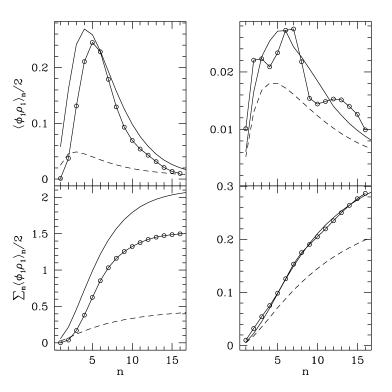
Figure 1: Top row: Fluctuation energy with orthogonal function index in units of background potential energy. Bottom row: Cumulative fluctuation energy with orthogonal function indices less than $n$. The left and right columns show the $l=m=1$ and $l=m=2$ harmonics respectively. The spatial profile of the potential functions is shown in Fig. 4 for $l=1,2$. The solid and dashed line follows from the analytic calculation for the self-gravitating response and Poisson fluctuations alone, respectively. The open circles are computed from the time-averaged expansion coefficients in the n-body simulation.

Figure 2: As in Fig. 1 but for the $l=m=3$ (left) and $l=m=4$ (right) harmonics.

Figure 3: Cumulative fluctuation energy for all harmonics of given $l$ (labeled) with orthogonal function indices less than $n$. Shown in units of background potential energy as in Fig. 1.

We will look at both King models and core-free Hernquist models. First, we apply equation (2.6) to a King model ($W_{0}=5$) for harmonics $l=m=1,2,3,4$ and compare with a SCF simulation for 100,000 particles and $l_{max}=4$. Figures 1 and 2 show the fluctuation energy per expansion function plotted against the index of expansion functions (cf. Fig. 4) and the cumulative fluctuation energy less than given index. One energy unit is equal to the total gravitational potential energy of the unperturbed sphere and ${\bar{m}}=1$. There are slight systematic differences between the n-body results and the predictions but all-in-all, the n-body simulation follows the analytic predictions fairly well and confirms the excess power at low order due to amplification by self gravity. This excess is illustrated in Figure 3 which shows the total energy for harmonic orders $l=1$–4 derived from the simulation. For $l=1$, the enhancement is roughly a factor of 6. The large magnitude for $l=1$ is due to the stochastic excitation of a weakly-damped mode. For $l=2$, the enhancement is roughly a factor of 1.5. For $l>4$ the power enhancement due to self gravity is negligible. The size of coherent structures decrease with increasing harmonic order and therefore higher harmonics have power at smaller and smaller scales for which self gravity is less important. The index at peak power increases with $l$ as expected.

The case for the core-free Hernquist model is shown in Figure 5 for harmonics $l=m=1,2$. The profiles are more sharply peaked about $n=1$ because the expansion functions well matched to the model profile (Hernquist & Ostriker 1992). Especially for the $l=m=1$ harmonic, the agreement between the expansion and the simulation is better in this case. This is probably due to the choice of expansion functions. For the $l=m=2$, the power appears systematically high at larger radial order. As for the King model, the power at $l=1$ has the largest enhancement by self-gravity, now by roughly a factor of 15 and this amplitude is verified by the simulation. The enhancement at $l=2$ is similar, roughly a factor of 1.5.

The root energy indicates the expected magnitude of the density or potential fluctuation and can be multiplied by $\sqrt{1/N}$ to estimate the magnitude for an $N$ particle simulation. For galaxian disk embedded in a massive halo, an large-scale $0.1\%$ distortion in the halo can have interesting consequences for disk evolution (cf. Weinberg 1997). In order to realistically test dynamical hypotheses for disk-halo interactions, we need to suppress noise below this level. This requires live halos with $N>10^{7}$ particles for S/N$>10$.

In particular, the fluctuating dipole ($l=1$) force field differentially accelerates and bends the disk, causing thickening. The quadrupole ($l=2$) in a arbitrary orientation warps the disk, causing the sort of warp discussed by Weinberg (1995, 1997) but now due to noise rather than a satellite wake. Even without self gravity, discreteness noise is sufficient to require $N>10^{6}$.

Figure 4: Potential functions used in fluctuation energy calculation in Fig. 1.

Figure 5: As in Figure 1 but for the Hernquist model.

4 Conclusions and discussion

This paper considers discreteness noise and its amplification in n-body simulations with particular attention a halo’s effect on an embedded disk. The overall conclusions are as follows:

1. The SCF n-body algorithm does not suppress Poisson fluctuations due to finite number of particles and Poisson fluctuations alone can result in significant distortions.

2. The low-order response is amplified by the coherent self-gravitating response of the entire system.

3. As discussed in Weinberg (1994), spherical systems have weakly damped modes at harmonics $l=m=1,2$. These are excited by noise and enhance the fluctuation power. This is clearly seen in Figures 1 and 5. Detailed agreement between the linearized solution and simulation reaffirms the importance of these modes to the self-gravitating response.

4. For $N$ particles, the $l=m=1(2)$ harmonics have roughly $4/N(1.5/N)$ times the energy of the background for the $W_{0}=5$ King model and $15/N(1.5/N)$ for the Hernquist model. The amplification does not rely on the existence of a core.

5. The noise amplitude in an n-body simulation with $N=10^{5}$ is comparable to the the amplitude required to produce a warp (Weinberg 1997). This analysis suggests simulations with $N\mathrel{\hbox{\hbox to0.0pt{\hbox{\lower 4.0pt\hbox{$\sim$}}\hss}\hbox{$>$}}}10^{7}$ will be necessary to achieve healthy a signal to noise ratio. Conversely, a halo with $N=10^{5}$ corresponds to masses of roughly 2 to $6\times 10^{6}{\rm\,M_{\odot}}$. This is comparable to the black hole mass required to produce the disk scale height by the Lacey & Ostriker (1985) mechanism. Fluctuations at this level are likely to excite bending modes in addition to increasing the disk scale height.

6. Although the fluctuations described in Figure 1 include self-gravity, self-gravity is a small ($<10\%$) perturbation for harmonics $l>4$.

The gravitationally amplified noise described here is unlikely to be a significant contribution to the overall evolution of a relaxing system, such as a globular cluster. However, the noise-excited $l=1$ structure may be sufficient to offset the cluster halo from its core. This could decrease the lifetime of any loss-cone population and subsequently decrease the rate of core cooling.

This calculation investigates the magnitude and nature of halo fluctuations assuming that the halo is an equilibrium phased-mixed distribution. However, the outer parts of galaxies can barely count 10 dynamical times so inhomogeneities will not have had time to phase mix and continued disturbance from mergers will not have relaxed (see Tremaine 1992 for additional discussion). It is likely that intrinsic fluctuations may play a significant role in long-term galaxian evolution. In particular, a companion paper (Weinberg 1997) elaborates the nature of satellite halo excitation and its role in producing warps using a similar formalism. N-body simulation of this process revealed that intrinsic noise had a similar effect on the disk. It is difficult to deduce the power produced by phase mixing streams based on the point-mass noise from $10^{5}$, $10^{6}$ or $10^{7}M_{\odot}$ fuzzy blobs and the degree of granularity will depend on the nature of the dark matter and halo formation history. Speculating further nonetheless, it is conceivable that a wide variety of observed disk structure such as arms and bars may have its roots in halo structure.

References

• [1] Clutton-Brock M., 1972, Astrophys. Space. Sci., 16, 101
• [2] Clutton-Brock M., 1973, Astrophys. Space. Sci., 23, 55
• [3] Edmonds A.Β R., 1960, Angular Momentum in Quantum Mechanics, Princeton University Press, Princeton, New Jersey
• [4] Gilbert I.Β H., 1968, ApJ, 152, 1043
• [5] Hernquist L., Ostriker J.Β P., 1992, ApJ, 386, 375
• [6] Krall N.Β A., Trivelpiece A.Β W., 1973, Principles of Plasma Physics, McGraw-Hill, New York
• [7] Lacey C.Β G., Ostriker J.Β P. 1985, ApJ, 299, 633
• [8] Nelson R.Β W., Tremaine S., 1997, Linear response, dynamical friction and the flucutation-dissipation theorem in stellar dynamics, preprint
• [9] Rostoker N., Rosenbluth M.Β N., 1960, Phys. Fluids, 3, 1
• [10] Tremaine S., 1992, in S.Β S. Holt, F. Verter (eds.), Back To The Galaxy, No. 278 in AIP Conference Proceedings, pp 599–609, American Institute of Physics
• [11] Tremaine S., Weinberg M.Β D., 1984, MNRAS, 209, 729
• [12] Weinberg M.Β D., 1989, MNRAS, 239, 549
• [13] Weinberg M.Β D., 1993, ApJ, 410, 543
• [14] Weinberg M.Β D., 1994, ApJ, 421, 481
• [15] Weinberg M.Β D., 1995, ApJL, 455, L31
• [16] Weinberg M.Β D., 1997, Dynamics of the galaxian disk, halo, and satellite interaction, preprint