Supersonic motions in dark clouds are not Alfvén waves

Abstract

Supersonic random motions are observed in dark clouds and are traditionally interpreted as Alfvén waves, but the possibility that these motions are super-Alfvénic has not been ruled out.

In this work we report the results of numerical experiments in two opposite regimes; $\beta\approx 1$ and $\beta\ll 1$, where $\beta$ is the ratio of gas pressure and magnetic pressure: $\beta=P_{g}/P_{m}$.

Our results, combined with observational tests, show that the model with $\beta\approx 1$ is consistent with the observed properties of molecular clouds, while the model with $\beta\ll 1$ has several properties that are in conflict with the observations.

We also find that both the density and the magnetic field in molecular clouds may be very intermittent. The statistical distributions of magnetic field and gas density are related by a power law, with an index that decreases with time. Magnetically dominated cores form early in the evolution, while later on the intermittency in the density field wins out.

1 Introduction

The observation of supersonic motions in molecular clouds (eg Zuckerman & Palmer 1974) raised the question of how these motions could be supported (Norman & Silk 1980; Fleck 1981; Scalo & Pumphrey 1982). Supersonic motions are expected to quickly dissipate their energy in highly radiative shocks, because of the very short cooling time of molecular gas or metal rich atomic gas (Mestel & Spitzer 1956; Spitzer 1968; Goldreich & Kwan 1974).

Strictly related was the issue of the support of molecular clouds (MCs) against gravitational collapse, since it was soon realized that the observed motions could not be understood as a gravitational collapse (Zuckerman & Evans 1974; Morris et al. 1974), although MCs contain many Jeans’ masses.

Theoreticians therefore formulated the hypothesis that MCs were primarily magnetically supported (Mestel 1965, Strittmatter 1966; Parker 1973; Mouschovias 1976a,b; McKee & Zweibel 1995) and interpreted the observed motions as long-wavelength hydro-magnetic waves (Arons & Max 1975; Zweibel & Josafatsson 1983; Elmegreen 1985, Falgarone & Puget 1986). It was also shown that the properties of the observed ‘turbulence’ (Larson 1981; Leung, Kutner & Mead 1982; Myers 1983; Quiroga 1983; Sanders, Scoville & Solomon 1985; Goldsmith & Arquilla 1985; Dame et al. 1986; Falgarone & Pérault 1987) could be understood if the motions were sub-Alfvénic (Myers & Goodman 1988; Mouschovias & Psaltis 1995, Xie 1996).

Nevertheless, recent attempts to detect the Zeeman effect, in lines of molecules such as OH and CN, that probe regions of dense gas (Crutcher et al. 1993; Crutcher et al. 1996), resulted in a number of non-detections of the effect, and therefore in rather stringent upper limits for the magnetic field strength, despite the fact that regions expected to favor detections were targeted. It is therefore possible, that the field strength in dense molecular gas is weaker than assumed in theoretical studies.

In the present work, we describe the dynamics of MCs, with the numerical solution of the equations of 3-D compressible magneto-hydrodynamics (MHD), in a regime of highly supersonic random motions. We avoid any sort of idealization of the physical system, apart from describing it as a fluid, and simply rely on the physical assumption (supported by the observations) that the motions in MCs are random. The main limitation of our numerical models, compared with MCs, is the absence of gravity. We have excluded gravity on purpose (our code is capable of handling self-gravity), because one of the aim of our work is to show that (magneto-)hydrodynamic processes alone are able to explain most of the observed properties of MCs, without the need of gravity. Although gravity is certainly responsible for the fragmentation into stars of high density regions, supersonic random motions shape the structure of molecular clouds with a minor contribution from gravity (Padoan 1995; Padoan, Jones & Nordlund 1997a; Padoan, Nordlund & Jones 1997b), apart from the possibility that gravity is the energy source of the motions on the large scale. The importance of supersonic motions in fragmenting the gas is certainly apparent on very small scales, where young and probably transient clumps are not originated by gravitational instability (Falgarone, Puget & Pérault 1992; Langer et al. 1995).

Previous numerical studies have shown that compressible turbulence can qualitatively explain several observational properties of MCs, even if the effect of gravity and magnetic fields are not included. The first two-dimensional (2-D) simulations of turbulence, with rms Mach number larger than one, were performed by Passot & Pouquet (1987). These were the first simulations where shocks are shown to develop inside a turbulent flow. The importance of shock formation inside mildly supersonic flows was later confirmed in 3-D simulations by Lee, Lele & Moin (1991). It was immediately recognized that shocks might have been responsible for the fragmentation of the density field inside MCs, and especially for the origin of their filamentary structure (Passot, Pouquet & Woodward 1988). Kimura & Tosa (1993) simulated the passage of a strong shock through a turbulent molecular cloud, and found that this process can generate dense clumps, with a power law mass spectrum. Vázquez-Semadeni (1994) made use of 2-D numerical simulations to show that supersonic turbulence generates a very intermittent density field, reminiscent of the clumpy nature of MCs. The density field was also found to be self-similar, which could be the reason for the hierarchical structure of MCs (Scalo 1985, Houlahan & Scalo 1992). Falgarone et al. (1994), analyzing the numerical simulation by Porter, Pouquet & Woodward (1994), argued that the properties of the profiles of molecular emission spectra from MCs can be interpreted as arising from turbulent motions.

Other numerical works included gravity in the turbulent flows, yet without describing the magnetic field. Turbulence was shown to be able to prevent gravitational collapse (cf Chandrasekhar 1958; Arny 1971; Bonazzola et al. 1987, 1992) in the 2-D numerical simulations by Léorat, Passot & Pouquet (1990). Vázquez-Semadeni, Passot & Pouquet (1995) modeled the galactic disc, on the scale of 1 Kpc, as a turbulent self-gravitating flow. They simulate a 2-D turbulent flow that is forced by the energy released by star formation (expansions of HII regions), and found that the main mechanism of cloud formation is the turbulent ram pressure, rather than gravity. They were not able to form self gravitating clouds, due to limitations in the thermal modeling, and the consequent low density contrast.

A 3-D description of a magnetized self-gravitating cloud was given by Carlberg & Pudritz (1990), and was used to simulate molecular emission spectra by Stenholm & Pudritz (1993). Carlberg & Pudritz found that the magnetic field and hydro-magnetic waves can support the cloud against gravity. The clouds contract, because of ambipolar diffusion, on a timescale of approximately four free-fall times. These simulations do not solve the MHD equations, but instead make use of a ’sticky particles’ code. Energy is injected in the form of a spectrum of Alfvén waves, and the outcome of the computation is dependent on the spectral index, that is a free parameter. This way of forcing the particles is rather unphysical, because an arbitrary spectrum of Alfvén waves is imposed, instead of being obtained as a result of the simulated magneto-hydrodynamics. Passot, Vázquez-Semadeni & Pouquet (1995) introduced the magnetic field in their previous 2-D model for the galactic disc (Vázquez-Semadeni, Passot & Pouquet 1995), and obtained a flow with rough equipartition of kinetic and magnetic energy, probably in rough equipartition also with the mean thermal energy. The same simulation, and others with larger density contrast and resolution, have been studied by Vázquez-Semadeni, Ballesteros-Paredes & Rodríguez (1997), who were able to reproduce the observed relation between line-width and size (Larson 1981). Gammie and Ostriker (1996) solved the MHD equations in a slab geometry, including self-gravity. By forcing the flow with a nonlinear spectrum of MHD waves, they were able to prevent the gravitational collapse of their 1-D cloud model.

Apart from the intentional exclusion of gravity, we have improved significantly on all previous calculations of turbulent flows. First of all we have solved the MHD equations in three-dimensions, while all previous solutions are in two or one dimensions. In MHD the dimensionality of the flow has a fundamental importance, because it determines the topological freedom of the magnetic field. Another improvement of our work is the high rms Mach number of the flows ($\sim$ 5), while previous models are only mildly supersonic (Mach number $\sim$ 1). While previous models of magnetized clouds focused on the role of the magnetic field as opposed to gravity, and therefore have assumed a magnetic pressure much larger than the gas pressure, the main purpose of the present work is to show that MCs are well described as flows with much lower magnetic pressure than previously assumed, and probably in rough equipartition with the gas pressure.

We report on the results of two numerical models. In model A, $\beta\approx 1$, in model B, $\beta\ll 1$, where $\beta$ is the ratio of gas pressure and magnetic pressure: $\beta=P_{g}/P_{m}$. The observations of magnetic field strengths are in agreement with a scenario where the mean magnetic pressure, $\langle B^{2}a\rangle$, is dynamically low (model A). Magneto-hydrodynamic (MHD) flows develop a very intermittent spatial distribution of the magnetic energy, and therefore, when the field is detected at a favorable position, its strength is far stronger than the mean field strength. Dense cores with sub-Alfvénic velocity dispersion can still be generated, in agreement with the observations.

2 The experiments

The study of the dynamics of MCs belongs to the field of random MHD flows, in a highly supersonic regime. The Reynolds number and the magnetic Reynolds number in MC flows are very large. Their random nature is therefore a basic feature of the dynamics of these flows, and requires an appropriate description.

For this reason, a realistic description of the dynamics of molecular clouds had to be based on the numerical solution of the compressible MHD equations in three dimensions, in a random and highly supersonic regime. We did it with relatively high resolution ($128^{3}$), with a code designed for turbulence and MHD turbulence experiments (Nordlund, Galsgaard & Stein 1994; Stein, Galsgaard & Nordlund 1994; Galsgaard & Nordlund 1996; Nordlund, Stein & Galsgaard 1996; Nordlund & Galsgaard 1997), specifically adapted to be able to deal with very strong shocks and very large density contrasts.

One of our purposes with these particular experiments is to explicitly address the classical arguments about dissipation time scales for super- and sub-Alfvénic motions, and we therefore perform the experiments in the spirit of “freely decaying turbulence”; studying the decay of an initial, solenoidal velocity field, without applying any external forcing. We include external forcing in other experiments that we have made (e.g., Padoan et al. 1997a, 1997b).

Although we have already developed a version of the code with the inclusion of the gravitational force, all the experiments were run without gravity, for the following reasons:

• We are mainly interested in studying the magneto-hydrodynamics, rather than the gravitational instability.

• The observed motions have velocities comparable with the virial velocity, or larger, on a range of scales, and the clouds are not free-falling.

• If the results of our experiments are discussed only up to a time shorter than or comparable to the dynamical (or free-fall) time, all our conclusions remain basically unchanged. This time is about a few million years on a scale of 10 pc, and clouds are not supposed to live much longer than that, before star formation takes place and becomes energetically important.

2.1 The equations

We solve the compressible MHD equations:

$${\partial\ln\rho\over\partial t}+{\bf v}\cdot\nabla\ln\rho=-\nabla\cdot{\bf v},$$ (1)

$${\partial{{\bf v}}\over\partial t}+{{\bf v}\cdot\nabla{\bf v}}=-{1\over\rho}\nabla P+{1\over\rho}{{\bf j}}\times{{\bf B}}+{\bf f},$$ (2)

$${\partial e\over\partial t}+{{\bf v}}\cdot\nabla e=-{P\over\rho}\nabla\cdot{{\bf v}}+Q_{\rm Joule}+Q_{\rm viscous}+Q_{\rm radiative},$$ (3)

$${\partial{{\bf B}}\over\partial t}=\nabla\times{\bf v}\times{\bf B},$$ (4)

$${\bf j}=\nabla\times{\bf B},$$ (5)

plus numerical diffusion terms, and with periodic boundary conditions. ${\bf v}$ is the velocity, ${\bf B}$ the magnetic field, ${\bf f}$ an external force ($=0$ in these particular experiments), and $p=\rho T$ is the pressure at $T\approx$ const.

Conditions in the cold molecular clouds that we are modeling are such that an isothermal approximation is adequate; the radiative heat exchange is so efficient that the temperature remains low in most places. Even if the temperature momentarily increases in shocks, the subsequent cooling is rapid, and the result is shock structures that are qualitatively and quantitatively similar to isothermal shocks.

We have thus used isothermal conditions in most of our runs and have verified that this is appropriate, by rerunning segments of some experiments using the full energy equation. No significant change of the statistics was found and, since using the full energy equation increases the cost of the experiments considerably (the strong cooling required to maintain a low temperature forces a much smaller time step), we performed most of the experiments at constant temperature.

The absence of an explicit resistivity $\eta$ in the induction equation corresponds to an assumption of flux freezing on well resolved scales. The code uses shock and current sheet capturing techniques to ensure that magnetic and viscous dissipation at the smallest resolved scales provide the necessary dissipation paths for magnetic and kinetic energy. As shown by Galsgaard & Nordlund (1976, 1977), dissipation of magnetic energy in highly turbulent MHD plasmas occurs at a rate that is independent of the details of the small scale dissipation. In ordinary hydrodynamic turbulence the corresponding property is one of the cornerstones of Kolmogorov (1941) scaling.

We have not included ambipolar diffusion in the present experiments, because it occurs on a time-scale significantly longer than the dynamical time, as recently shown by Myers & Khersonsky (1995) and is thus expected to be of secondary importance. However, our code has the ability to handle ambipolar diffusion, and we plan to study its effects in a subsequent paper.

2.2 The code

The code solves the compressible MHD equations on a 3D staggered mesh, with volume centered mass density and thermal energy, face centered velocity and magnetic field components, and edge centered electric currents and electric fields (Nordlund, Stein & Galsgaard 1996).

The original code works with “per-unit-volume” variables; mass density, momenta, and thermal energy per unit volume. In the super-sonic regime relevant in the present application, we found it advantageous to rewrite the code in terms of “per-unit-mass” variables; $ln\rho$, $u$, and $E=\frac{3}{2}\frac{P}{\rho}$. With these variables, the time evolution of all variables is governed by equations of the type

$${Df\over Dt}={\partial f\over\partial t}+{\bf v}\cdot f=...;$$ (6)

i.e., equations that specify the time rate of change following the motion. These are better conditioned than the divergence type equations that result from using per-unit-volume variables (the large—order $M^{2}$— density variation in isothermal shocks cause the per-unit-volume fluxes to vary over several orders of magnitude).

We use spatial derivatives accurate to 6th order, interpolation accurate to 5th order, and Hyman’s 3rd order time stepping method (Hyman 1979).

In order to minimize the viscous and resistive influence on well resolved scales, we use monotonic 3rd order hyper-diffusive fluxes instead of normal diffusive fluxes, and in order to capture hydrodynamic and magneto-hydrodynamic shocks we add diffusivities proportional to the negative part of the velocity divergence, and resistivity proportional to the negative part of the cross-field (two-dimensional) velocity divergence. Further details of the numerical methods are given by Nordlund, Galsgaard & Stein (1996) and Nordlund & Galsgaard (1997).

2.3 Weak and strong magnetic field

For the purpose of this work we have run two experiments: one with $\beta_{i}=4$ (model A), and the other with $\beta_{i}=0.04$ (model B), where $\beta_{i}=(P_{g}/P_{m})_{i}$ is the initial ratio of gas and magnetic pressure.

In both experiments the initial density is uniform, and the initial velocity is random. We generate the velocity field in Fourier space, and we give power, with a normal distribution, only to the Fourier components in the shell of wave-numbers $1<k<2$. We perform a Helmholtz decomposition, and use only the solenoidal component of the initial velocity. The initial magnetic field is uniform, and is oriented parallel to the $z$ axis: ${\mathbf{B}}=B_{0}{\mathbf{\hat{}}{z}}$.

In experiment B, the initial velocity field is perpendicular to the magnetic field (zero $z$ component), in order to excite the Alfvén waves, while in experiment A the initial velocity field has equal amplitude in all three components. Both experiments are decaying flows, because no external forcing is applied.

We define the Alfvénic Mach number, ${\cal{M}}_{A}$, as the ratio of the flow rms velocity and the Alfvén velocity. In model A, ${{\cal{M}}_{A}}\approx 10$, and in model B, ${\cal{M}_{A}}\approx 1$, initially. Under isothermal conditions, in our units, the ordinary Mach number ${\cal{M}}={\cal{M}}_{A}/\beta^{1/2}$, so the ordinary Mach number is initially ${\cal{M}}\approx 5$ in both cases.

Fig. 1 shows the time evolution of the rms Mach number and rms density in the two experiments. In both cases, the rms density grows to the value $\sigma_{n}\approx 0.5{\cal{M}}$, where ${\cal{M}}$ is the rms Mach number of the flow, in about one dynamical time, defined as the ratio of half the linear size of the box over the initial rms velocity, $t_{dyn}=0.5L_{box}/\sigma_{v,0}$.

The initial Mach number in experiment B is a bit smaller than in experiment A, because the amplitude of the initial $z$ component of the velocity field is zero. Nevertheless, energy is immediately transferred to the $z$ component of the velocity, and the rms $z$ component is subsequently about half the value of the other two components.

Fig. 2 illustrates the time evolution of the kinetic and magnetic energies, expressed in units of the mean thermal energy. The time evolution of the magnetic energy is totally different in the two experiments. In model B the field lines are only weakly perturbed by the flow, and exchange their energy with the flow periodically (oscillations in magnetic and kinetic energy, $E_{m}$ and $E_{k}$); in model A, instead, the magnetic field is almost passively advected, and its intensity and direction are strongly influenced by compressions and stretching of field lines. $E_{m}$ grows until it is in approximate equipartition with the thermal energy of the gas, but remains well below equipartition with the kinetic energy.

3 Observational tests

In this section we compare our numerical results with observed properties of molecular clouds.

3.1 Dissipation of supersonic motions

The time evolution of the kinetic energy is plotted in Fig. 2. After two dynamical times, $t=2.0t_{dyn}$, the flow in experiment A still contains about $30\%$ of its initial kinetic energy or, in other words, the rms velocity is still about $55\%$ of its initial value. In experiment B, the mean kinetic energy of the oscillations after two dynamical times is about $40\%$ of its initial value, i.e. the rms velocity is about $63\%$ of the initial value.

Thus, contrary to the beliefs that partly motivated developing the Alfvén wave model of MC turbulence, the dissipation in model A is not particularly rapid in absolute terms, and the dissipation in model B is not particularly small. Thus, the advantage of the Alfvén wave model, as far as the energy dissipation time-scale is concerned, is little: $t_{diss,B}=1.3t_{diss,A}$. Although this was already appreciated in Zweibel & Josafatsson (1983) and Elmegreen (1985), it should be noticed that here we do not include the dissipation mechanism of ion-neutral friction. Alfvén waves dissipate mainly because they transfer their energy to motions along the magnetic field, that are eventually dissipated in shocks. This was found also by Gammie and Ostriker (1996). It is clear therefore that, from the point of view of the dissipation mechanism, model B is not significantly superior to model A.

The dissipation of the supersonic motions is not a problem for any of the models, however, because:

• If motions are present there must be a source for their energy; such a source may be active for more than one dynamical time.

• After one dynamical time $50\%$ of the initial energy in model A is still in the flow. At the scale of $10$ pc the dynamical time is about $3\times 10^{6}$ years: clouds do not need to exist much longer than that before star formation significantly affects their energetics (Blitz & Shu 1980).

3.2 Magnetic energy probability distribution

We illustrate the probability distribution of the magnetic energy in units of the mean thermal pressure: $1/\beta=B^{2}/<P_{g}\rangle$. We recall that initially $\beta$ is uniform in both models, and its value is $\beta_{i}=4$ in model A, and $\beta_{i}=0.04$ in model B.

The distribution of the magnetic energy is shown in Fig. 3. Model A develops a very intermittent distribution, with an exponential tail.

Taking into account the relation between field strength and density (see next section), one finds that approximately $0.5\%$ of the total mass of the system contains a field 10 times stronger than the mean value. For example, in a cloud of $10^{4}M_{\odot}$, one can find a couple of clumps of about $30M_{\odot}$ each, with a field strength $B=40\mu G$, while the mean field of the cloud is only $B=4\mu G$.

Model B is much less intermittent than model A.

3.3 The relation B-n

In regions of maser emission, at densities of about $n=10^{7}cm^{-3}$, a field strength of the order of $B=10^{3}-10^{4}\mu G$ is observed, while in regions of molecular emission, with approximately $n=10^{2}-10^{3}cm^{-3}$, the field is found to be of the order of $B=10\mu G$ (eg Myers & Goodman 1988).

A relation of the type $B\propto n^{0.3-0.6}$ may be deduced from the observations (eg Troland, Crutcher & Kazès 1986; Heiles 1987; Dudorov 1991), but it is quite uncertain, especially in the light of the above discussion about the intermittency of the distribution of the magnetic energy.

The fact remains, however, that observationally the field strength certainly grows with the gas density, and this is found over a range of 6 orders of magnitudes in density, and 3 orders of magnitude in field strength.

Fig. 4 shows the relation $B-n$ in models A and B. The dispersion in the relation $B-n$ is shown in the form of $1-\sigma$ ‘error’ bars in the plot of Fig. 4. In model A the slope of the relation decreases with time. We find $B\propto n^{0.8}$ at $t=0.2t_{dyn}$, $B\propto n^{0.7}$ at $t=1.0t_{dyn}$, $B\propto n^{0.5}$ at $t=2.0t_{dyn}$, and $B\propto n^{0.3}$ at $t=3.0t_{dyn}$. We interpret this time evolution of the relation $B-n$ in the next section.

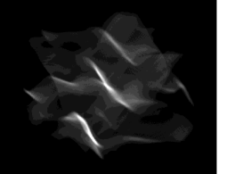
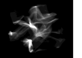
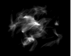
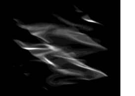
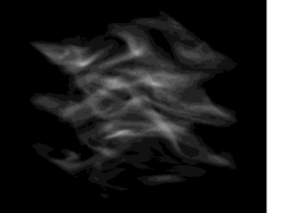
Figure 5: 3-D representation of the time evolution of the density field. Time evolves from left to right. The upper row of panels show model A, while the lower row shows model B.

In model B there is no significant correlation between $B$ and $n$. The lack of correlation between $B$ and $n$ was to be expected: most of the density enhancement occurs by convergent flows along the field lines, in the $z$ direction, and these motions do not affect the magnetic field. A nice illustration of this is provided by the snapshots in Fig. 5 (lower row), where the density field is stratified in planes that are predominantly perpendicular to the $z$ direction (vertical direction in the images). The densest regions develop at nodes in the large-scale waves, as found by Carlberg & Pudritz (1990).

One could possibly argue that the lack of correlation of $B$ and $n$ is consistent with the majority of observations, because no field is detected, and hence nothing can be said about the correlation. However, as further discussed in Section 4 below, the upper limits of the non-detections speak against this interpretation. Also, the cases where a field is detected would then have to be explained with ad hoc arguments, rather than as a natural part of a statistical distribution.

An interesting consequence of the model A results is that the observed relation could in principle be used to set an independent estimate of the age of molecular clouds: the comparison between model A and the observations would indicate that molecular clouds, on the average, have survived, since they were almost uniform in density and field distribution, for 2 or 3 dynamical times, that is about $10^{7}$ years, on a scale of $20$ pc. This estimate has little to do with the estimate of the time-scale for massive stars to destroy the parent molecular cloud (Blitz & Shu 1980), since that calculation has nothing to say about the lifetime of the cloud after it cooled from diffuse warm gas.

To conclude, note that Fig. 4 illustrates that, even if in model A the mean magnetic field is such that the $\langle\beta\rangle\approx 0.7$, in regions only 10 times denser than the mean, the field can be as intense as in model B.

3.4 Cloud and flow topology

An understanding of the spatial structure of the density field in dark clouds is very important for a correct interpretation of observational data, and for the formulation of a number of physical models.

The snapshots in Fig. 5 give an idea of the dimensionality of the structures in the density field. It is apparent that experiment B (lower row of panels) develops a stratified density field, with sheet-like structures, the sheets being approximately perpendicular to the magnetic field (the $z$ direction corresponds to the vertical direction in the figures). This is consistent with the fact that only the motions in the $z$ direction can compress the gas to very high density.

The topology of the density field in experiment A (upper row of panels in Fig. 5) has a clear evolution in time. In the very beginning, until $t\approx 0.4t_{dyn}$, the density grows predominantly in sheets. These are the fronts of blobs of coherent motion, advancing at supersonic velocity. Later, these fronts start to intersect each other, and the density increases especially in filaments (at the intersections of fronts). The evolution continues with the intersection of filaments into knots, at $t\approx 1.5t_{dyn}$. The fully developed topology, at $t=2.0t_{dyn}$, is characterized by both filaments and knots (cores).

The evolution of the magnitudes of the mass density and the magnetic field may be discussed with reference to Lagrangian version of the continuity equation,

$${{\rm D}\ln\rho\over{\rm D}t}=-\nabla\cdot{\bf v},$$ (7)

and the scalar induction equation

$${{\rm D}\ln|B|\over{\rm D}t}=-\nabla_{\perp}\cdot{\bf v},$$ (8)

where $\nabla_{\perp}\cdot$ stands for the divergence perpendicular to the magnetic field, following both the motion and the change of orientation of the field lines.

Although $-\nabla\cdot{\bf v}$ vanishes for the solenoidal initial condition, the supersonic motions rapidly lead to the formation of shock fronts, where the local value of $-\nabla\cdot{\bf v}$ is large and positive because of the discontinuity in the velocity perpendicular to the shock.

The initially homogeneous magnetic field is carried along by the perpendicular components of the velocity field, and is hence also collected into sheets, except at those rare locations where the initial field happens to be strictly parallel to the velocity field. This explains why sheets initially form in both mass density and magnetic flux density, and why the $B-n$ relation initially has an exponent close to unity.

Note that the usual argument for a slope of 2/3, that applies to isotropic and non-shocking compressible motion does not apply here, because of the development of discontinuities. In term of Eqs. 7 and 8, the 2/3 follows if $-\nabla_{\perp}\cdot{\bf v}$ typically picks up two of the three directional contributions to $-\nabla\cdot{\bf v}$. However, at a shock, the divergence is dominated by the derivative in one particular direction; the one perpendicular to the shock front. The magnetic field that is swept into the discontinuity quickly becomes almost parallel to the shock front, because the component in the plane of the shock grows exponentially with time. Thus, as long as the topology is dominated by sheets, the mass density and the magnetic flux grow more or less in unison in the sheets, corresponding to an exponent in the $B-n$ relation close to unity.

In the subsequent evolution, there are effects that tend to reduce the exponent in the $B-n$ relation. First, the non-linear evolution of the initially solenoidal velocity field also leads to the development of regions of space with a positive divergence, in which both the mass density and the magnetic flux density decline. In these regions, there is no particular dominance of the cross-field divergence, and thus the three-dimensional divergence picks up un additional contribution relative to the two-dimensional divergence, consistent with the classical 2/3 argument outlined above.

In experiment B the motions are mainly Alfvén waves, and therefore the velocity is predominantly perpendicular to the direction of the magnetic field. This is illustrated in Fig. 6, where we have plotted the histogram of $cos(\alpha)$, where $\alpha$ is the angle between ${\bf v}$ and ${\bf B}$. Note that, even though motions across the field lines are the most common ones, it is the less frequent motions along the field lines that dominate the dissipation, as mentioned in connection with the discussion of Fig. 5 above. The motions across field lines are subject to magnetic restoring forces, and do not lead to density enhancements. It is the motions along the field lines that lead to the sheet like density enhancements visible in Fig. 5.

In experiment A, the magnetic field is advected by the flow, and the stretching of field lines instead produces some alignment between ${\bf v}$ and ${\bf B}$, already before one dynamical time has passed, as illustrated in Fig. 6.

Alignment between ${\bf B}$ and ${\bf v}$ may be caused by two, complementary effects: 1) Dynamical alignment is expected when the magnetic energy approaches and exceeds the kinetic energy; the Lorentz force then forces the flow to be predominantly along the magnetic field lines. 2) Kinematic alignment occurs when a spatially non-uniform velocity field causes stretching of magnetic field lines, and hence a correlation of ${\bf B}$ and ${\bf v}$. Pure shear, for example, tends to align an embedded magnetic field with the direction of the flow.

Motions that are aligned with the magnetic field affect the mass density without affecting the magnetic flux density. In particular, the non-linear concentration into first sheets and then filaments due to the interaction of shock fronts continues into the formation of knots in the density field, by the convergence of matter flowing along filaments. There is no corresponding process available to a divergence free vector field such as the magnetic field; once the field has concentrated into filaments, it cannot concentrate further; the magnetic field in a filament is insensitive to flow along the filament.

In the same way that converging flows along the magnetic field may lead to extreme concentrations of mass, those regions where the flow is diverging along magnetic field lines may lead to extreme rarefactions of mass, without affecting the magnetic flux density. In $B-n$ scatter plots, this corresponds to the development of more extreme excursions of the mass, relative to those of the magnetic flux density, and hence a flattening of the $B-n$ relation with time.

In model A, dynamical alignment is at most significant in the few cores that develop a strong (sub-Alfvénic) magnetic field in the early evolution of the experiment. In scatter plots of $B$ against $n$ most contributions come from regions where dynamical alignment is unimportant. We thus conclude that the evolution of the $B-n$ relation in model A, towards a smaller exponent with time, is caused by the kinematic alignment of ${\bf B}$ and ${\bf v}$.

3.5 Stellar extinction

Padoan, Jones, & Nordlund (1997) have shown that near-infrared stellar extinction determinations can be used to infer the 3-D probability distribution of the gas density in dark clouds. They have shown that there is qualitative and quantitative agreement between the inferred 3-D density distribution in dark clouds, and the one produced by their experiment of random supersonic flows.

The method is based on the plot of the dispersion of the extinction measurements in cells, versus the mean extinction in the same cells (Lada et al. 1994). In Padoan, Jones & Nordlund (1997), the theoretical plots are produced by generating random density fields of given statistics and power spectra. Here we show one example of the same plot, but produced directly from the density field of experiments A and B. The plot is shown in Fig. 7, that can be compared directly with the plots shown in Padoan, Jones, & Nordlund. The plot of model A looks like the observational one. It has a smaller slope because the rms Mach number in Experiment A is smaller than in the observed cloud.

The plot for Experiment B seems instead to differ from the observational one. The absence of locations with very low extinction in model B is due to the fact that the density field in experiment B is mainly organized in sheets, perpendicular to the magnetic field direction.

4 Discussion

It is difficult to get an objective view on the magnetic field strength in dark clouds from the literature. The reasons are the following:

• Negative results from observational programs, in which detections have been reported, often remain unpublished.

• The positions searched for Zeeman splitting never represent a statistically meaningful sample. Favorable regions are always selected, because the observations are very time consuming.

• The total number of regions in dark clouds, for which OH Zeeman observations are published, is still small.

The best study of OH Zeeman splitting in dark clouds we are aware of is by Crutcher et al. (1993). They selected 4 cores in the Taurus dark cloud complex, 2 in the Libra complex, 2 in $\rho$ Oph, 1 in the Orion molecular ridge, 1 position in L889, and the core of B1 (Barnard 1), in the Perseus region. The only certain detection is in the cloud B1. For the other regions, the weighted average value of the field is $+2.7\pm 1.5\mu G$ in Taurus, $-2.1\pm 2.8\mu G$ in Libra, $+6.8\pm 2.5\mu G$ in $\rho$Oph, $-0.6\pm 2.1\mu G$ in L889, and $-4.7\pm 3.5\mu G$ in L1647.

Two well known regions of very intense magnetic field are Orion A and Orion B. OH Zeeman splitting in Orion A revealed a magnetic field strength of $B=-125\mu G$ (Troland, Crutcher, & Kazès 1986), and $B=+38\mu G$ toward Orion B (Crutcher, & Kazès 1983).

Crutcher et al. (1996) have reported the first attempt to measure CN Zeeman splitting. They observed towards the cores OMC-N4 and S106-CN. They did not detect the magnetic field, and their upper limits are several times smaller than the value expected if the observed motions were sub-Alfvénic.

An average field of $+9\mu G$ was found in Cas A by Heiles and Stevens (1986).

The OH Zeeman splitting should probe regions with $n=10^{3}-10^{4}$ cm^-3, while the CN Zeeman splitting, should probe regions of $n\approx 10^{6}$ cm^-3.

Note that all works are biased toward regions of strong field, because only regions considered to be favorable for magnetic field detections are selected for Zeeman splitting observations. Despite that, in many cases the field is not detected, and upper limits are quite stringent.

In our model A we find that, if the mean field strength is $\langle B^{2}\rangle^{1/2}=5\mu G$, and the mean density $\langle n\rangle=10^{3}cm^{-3}$, at the time $t=2.0t_{dyn}$, then $20\%$ of the total mass is in dense clumps, with density ten times larger than the mean, $n\approx 10^{4}cm^{-3}$, and field strength five times, or more, larger than the mean, $B\geq 25\mu G$. Therefore, even if field strengths of about $30\mu G$ are detected sometimes in dense cores, the mean Alfvén velocity in the molecular cloud may be just comparable to the sound speed, $\langle v_{A}^{2}\rangle^{1/2}\approx C_{S}$.

On the basis of the observational results by Crutcher et al. (1993, 1996), it may be concluded that model A is in consistent with the observational estimates of magnetic field strength in dark clouds. The particular values of the magnetic field used in the comparison here should not be taken too literally; the small scale field strengths could be larger than estimated by the Zeeman effect if the magnetic field is tangled.

It is difficult to envisage how the measurements could be consistent with model B, however, since the magnetic field in a sub-Alfvénic model by definition has an energy that exceeds the kinetic energy. As demonstrated by Galsgaard & Nordlund (1996), a magnetically dominated plasma is able to quickly dissipate structural complexity, independent of the value of the resistivity. Thus, a sub-Alfvénic field could not remain strongly tangled, and hence could not avoid detection. Using the same argument, we expect those cores where a strong (sub-Alfvénic) field has indeed been observed to have a relatively simple magnetic field structure.

Model A can be used for the description of a typical molecular cloud with linear size of about $5$ pc and $\langle n\rangle=500$ cm^-3. At the time $t=1.0t_{dyn}$, the relation $B-n$ is then:

$$B=5\mu G(\frac{n}{500cm^{-3}})^{0.7}$$ (9)

Since the exponent is $>0.5$, most of the dense cores are found to have magnetic pressure larger than thermal pressure, at early times. This is illustrated in Fig. 8, where we have plotted the Alfvén velocity versus the gas density, after one dynamical time, for experiments A and B. In model A, one can see that, on average, regions with density larger than the mean are characterized by an Alfvén velocity larger than the sound velocity, and therefore by a magnetic pressure larger than the thermal pressure.

The lowering of the exponent in the $B-n$ power law with time means that later on, the dominance of the magnetic field in these cores tends to be reduced. Although the flow is random and approximately isotropic, the kinematic alignment of ${\bf B}$ with ${\bf v}$ makes dense cores accrete mass along ${\bf B}$ at an increased rate. Therefore, the accretion of mass around dense cores, embedded in a random flow with $\beta\approx 1$, is such that, while magnetic pressure becomes dominant over thermal pressure during the initial phase of fragmentation, later on magnetic pressure decreases to the level of thermal pressure, even in the absence of gravity, and on a timescale that is competitive with ambipolar diffusion. This mechanism could be relevant for the process of star formation.

The main point we want to clarify in this paper is that the fact of finding some cloud cores, with sub-Alfvénic velocity dispersions and with magnetic pressure larger than thermal pressure, does not necessarily mean that the dynamics of molecular clouds is dominated by MHD waves; those cores may be formed, in a few million years, in a supersonic and super-Alfvénic flow, only marginally affected by the magnetic field (model A). The dynamics becomes strongly affected by the magnetic field only in some very dense regions, on small scales, and at early times.

We stress that a key theoretical ingredient to the interpretation of OH Zeeman splitting data is the $B-n$ relation. The fact that the exponent of the relation is $>0.5$ for more than two dynamical times is the reason why sub-Alfvénic cores can be found in the experiment.

5 Conclusions

In this work we have shown that:

• Supersonic motions in model A are relatively long-lived, with decay times comparable to the estimated life-time of molecular clouds. Even in the absence of an energy source, supersonic and super-Alfvénic motions can persist as such, on a scale of $20$ pc, for about $10^{7}$ years.

• Supersonic sub-Alfvénic motions (model B) dissipate their energy almost as fast as super-Alfvénic motions. The original motivation for the MHD wave model is therefore absent.

• Random supersonic motions produce a very intermittent probability distribution of the magnetic energy, with an exponential tail. Since the distribution is so intermittent, one could easily detect a field strength that is several times in excess of the mean strength.

• Dense cores, with magnetic pressure larger than thermal pressure, and velocity dispersions smaller than $v_{A}$, are found as the result of the evolution of supersonic and super-Alfvénic flows (model A).

• A power law statistical $B-n$ relation is generated by supersonic motions, in model A, but not by MHD waves, in model B. The exponent of the relation is $>0.5$ for about two dynamical times, which allows for the existence of cores with $v_{A}>C_{S}$.

• The exponent in the $B-n$ relation decreases with time, because magnetic field lines are stretched and partially aligned with the flow. The statistical importance of the magnetic pressure in dense cores is thus expected to decrease with time, even in the absence of gravity and ambipolar diffusion.

• The topology of the density field generated by model A is mainly filamentary and clumpy. This is reminiscent of the morphology of molecular clouds. On the other hand, the density field produced by MHD waves in model B is mainly structured in sheets, perpendicular to the magnetic field.

• The statistical properties of the density field generated by random supersonic motions (as in model A) are in agreement with the statistical properties of the gas density in dark clouds, as inferred from stellar extinction determinations. Model B does not give such a good agreement.

The comparison between model A and model B shows that model A (super-Alfvénic motions) provides a nice understanding of the dynamics and structure of molecular clouds. Moreover, it is consistent with the OH Zeeman detections.

We conclude that the supersonic motions observed in dark clouds, on a scale of a few parsecs to several parsecs, can be understood, without any major problem, as super-Alfvénic motions, although sub-Alfvénic dense cores certainly exist.

Figure 1: Time evolution of rms Mach number and rms number density.

Figure 2: Time evolution of kinetic and magnetic energies, in units of the mean thermal energy.

Figure 3: Distribution of magnetic energy in units of the mean gas pressure, after one dynamical time. The dotted vertical line marks the initial mean value of the magnetic energy, and the dashed line the mean value after one dynamical time.

Figure 4: The relation $B-n$, after one dynamical time. The magnetic field is expressed in the numerical units, that is as an Alfvén velocity (defined with the mean gas density), in units of the sound speed. The $1-\sigma$ ‘error’ bars show the dispersion of values of $B$ around the mean for each bin. The size of the bins is chosen in order to have the same number of measurements inside each bin.

Figure 6: Histograms of the cosine of the angle between ${\bf v}$ and ${\bf B}$. In experiment A there is a partial alignement, while in experiment B the two fields are mainly perpendicular to each other.

Figure 7: Relation between the dispersion of the extinction and the mean extinction, on a regular grid superposed of the projection of the density field. The value of the extinction are measured at random positions, simulating the random position of a star behind the cloud.

Figure 8: The Alfvén velocity, in units of the sound velocity, versus the gas density. The dashed line is the $B-n$ relation, that is to say the Alfvén velocity defined with the mean density, instead of with the local density. In Experiment A, the magnetic pressure is on average larger than the gas pressure, in regions with gas density larger than the mean.

References

- (1) Arny, T. 1971, ApJ, 169, 289
- (2) Arons, J. & Max, C. E. 1975, ApJ, 196, L77
- (3) Blitz, L. & Shu, F. H. 1980, ApJ, 238, 148
- (4) Bonazzola, S., Falgarone, E., Heyvaerts, J., Perault, M. & Puget, J. L. 1987, A&A, 172, 293
- (5) Bonazzola, S., Perault, M., Puget, J. L., Heyvaerts, J., Falgarone, E. & Panis, J. F. 1992, J. Fluid Mech., 245, 1
- (6) Carlberg, R. G. & Pudritz, R. E. 1990, MNRAS, 247, 353
- (7) Chandrasekhar, S. 1958, Proc. Roy. Soc., 246, 301
- (8) Crutcher, R. M. & Kazès, I. 1983, A&A, 125, L23
- (9) Crutcher, R. M., Troland, T. H., Goodman, A. A., Heiles, C., Kazès, I. & Myers, P. C. 1993, ApJ, 407, 175
- (10) Crutcher, R. M., Troland, T. H., Lazareff, B. & Kazès, I. 1996, ApJ, 456, 217
- (11) Dame, T. M., Elmegreen, B. G., Cohen, R. S., Thaddeus, P. 1986, ApJ, 305, 892
- (12) Dudorov, A. E. 1991, Sov. A., 35(4), 342
- (13) Elmegreen, B. G. 1985, ApJ, 299, 196
- (14) Falgarone, E. & Puget, J. L. 1986, A&A, 162, 235
- (15) Falgarone, E., Pérault, M. 1987, in Physical Processes in Interstellar Clouds, ed. G. Morfil, M. Scholer (Dordrecht: Reidel), 59
- (16) Falgarone, E., Puget, J., -L. & Pérault, M. 1992, A&A, 257, 715
- (17) Falgarone, E., Lis, D. C., Phillips, T. G., Pouquet, A., Porter, D. H. & Woodward, P. R. 1994, ApJ, 436, 728
- (18) Fleck, R. C. Jr 1981, ApJ, 246, L151
- (19) Galsgaard, K. & Nordlund, Å. 1996, J. of Geophys. Res., 101(A6),13445
- (20) Galsgaard, K. & Nordlund, Å. 1997, J. of Geophys. Res., 102, 231
- (21) Gammie, C. F. & Ostriker, E. C. 1996, ApJ, 466, 814
- (22) Goldreich, P. & Kwan, J. 1974, ApJ, 189, 441
- (23) Goldsmith, P. F. & Arquilla, R. 1985, in Protostars and Planets II, University of Arizona Press, p. 137
- (24) Heiles, C., Stevens, M. 1986, ApJ, 301, 331
- (25) Heiles, C. 1987, D. J. Hollenbach & H. A. Thronson (eds.), Interstellar Processes, Reidel, p. 171
- (26) Houlahan, P. & Scalo, J. 1992, ApJ, 393, 172
- (27) Hyman, J. M. 1979, R. Vichnevetsky & R. S. Stepleman (eds.), in Adv. in Comp. Meth. for PDE’s, p. 313
- (28) Kimura, T. & Tosa, M. 1993, ApJ, 406, 512
- (29) Kolmogorov, A. N. 1941, Dokl. Akad. Nauk. SSSR, 30, 301–305.
- (30) Lada, C. J., Lada, E. A., Clemens, D. P., & Bally, J. 1994, ApJ, 429, 694
- (31) Langer, W. D., Velusamy, T., Kuiper, T. B. H., Levin, S., Olsen, E., Migenes, V. 1995, ApJ, 453, 293
- (32) Larson, R. B. 1981, MNRAS, 194, 809
- (33) Lee, S., Lele, S. K., Moin, P. 1991, Phys. Fluids A 3, 657
- (34) Léorat, J., Passot, T., Pouquet, A. 1990, MNRAS, 243, 293
- (35) Leung, C. M., Kutner, M. L., Mead, K. N. 1982, ApJ, 262, 583
- (36) McKee, C. F. & Zweibel E. G. 1995, ApJ, 440, 686
- (37) Mestel, L. & Spitzer, L. 1956, MNRAS, 116, 503
- (38) Mestel, L. 1965, Q. Jl. R.A.S., 6, 161, 265
- (39) Morris, M., Zuckerman, B., Turner, B. E. & Palmer, P. 1974, ApJ, 192, L23 ıı
- (40) Mouschovias, T. Ch. 1976a, ApJ, 206, 753
- (41) Mouschovias, T. Ch. 1976b, ApJ, 207, 141
- (42) Mouschovias, T. Ch. & Psaltis, D. 1995, ApJ, 444, L105
- (43) Myers, P. C. 1983, ApJ, 270, 105
- (44) Myers, P. C. & Goodman, A. A. 1988, ApJ, 326, L27
- (45) Myers, P. C. & Khersonsky, V. H. 1995, ApJ, 442, 186
- (46) Nordlund, Å, Galsgaard, K. & Stein, R. F. 1994, in R, J, Rutten, C J. Schrijver (eds.), Solar Surface Magnetic Fields, Vol. 433, NATO ASI Series
- (47) Nordlund, Å, Stein, R. F. & Galsgaard, K. 1996, in J. Wazniewski (ed.), Proceedings from the PARA95 workshop, Vol 1041 of Lecture Notes in Computer Science, p. 450
- (48) Nordlund, Å& Galsgaard, K. 1997, Journal of Computational Physics, (in preparation)
- (49) Norman, C., Silk, J. 1980, ApJ, 238, 158
- (50) Padoan, P. 1995, MNRAS, 277, 377
- (51) Padoan, P., Jones, B. J. T. & Nordlund, Å. 1997, ApJ, 474, 730
- (52) Padoan, P., Nordlund, Å. & Jones, B. J. T. 1997, MNRAS, in press
- (53) Parker, D. A. 1973, MNRAS, 163, 41
- (54) Parker, E. N. 1994, Spontaneous Current Sheets in Magnetic Fields, Oxford University Press
- (55) Passot, T., Pouquet, A. 1987, J. Fluid Mech., 181, 441
- (56) Passot, T., Pouquet, A., Woodward, P. 1988, A&A, 197, 228
- (57) Passot, T., Vázquez-Semadeni, E. & Pouquet A. 1995, ApJ, 455, 536
- (58) Porter, D. H., Pouquet, A. & Woodward, P.R. 1994, Phys. Fluids, 6, 2133
- (59) Quiroga, R. J. 1983, Ap. Sp. Sci., 93, 37
- (60) Sanders, D. B., Scoville, N. Z., Solomon, P. M. 1985, ApJ, 289, 372
- (61) Scalo, J. M., Pumphrey, W. A. 1982, ApJ, 258, L29
- (62) Scalo, J. M. 1985, in Protostars and Planets II, ed. D. C. Black and M. S. Mathews (Tucson: University of Arizona Press), 349
- (63) Spitzer, L. 1968, in Nebulae and Interstellar Matter, Stars and Stellar Systems, ed. B. Middlehurst, L. H. Aller, 7, 1, Univ. Chicago Press
- (64) Stein, R. F., Galsgaard, K. & Nordlund, Å. 1994, in J. D. B. et al (ed.), Proc. of the Cornelius Lanczos International Centenary Conference, Society for Industrial and Applied Mathematics, Philadelphia, p. 440
- (65) Stenholm, L. G. & Pudritz, R. E. 1993, ApJ, 416, 218
- (66) Strittmatter, P. A. 1966, MNRAS, 132, 359
- (67) Troland, T. H., Crutcher, R. M. & Kazès, I. 1986, ApJ, 304, L57
- (68) Vázquez-Semadeni, E. 1994, ApJ, 423, 681
- (69) Vázquez-Semadeni, E., Ballesteros-Paredes, J. & Rodríguez, L. F. 1997, ApJ, 474, 292
- (70) Vázquez-Semadeni, E., Passot, T. & Pouquet, A. 1995, ApJ, 441, 702
- (71) Velusamy, T., Kuiper, T. B. H., Langer, W. D., in preparation
- (72) Zuckerman, B. & Evans, N. J. 1974, ApJ, 192, L152
- (73) Zuckerman, B. & Palmer, P. 1974, ARA&A, 12, 279
- (74) Zweibel, E. G. & Josafatsson, K. 1983, ApJ, 270, 511
- (75) Xie, T. 1997, ApJ, 475, L139