A Theoretical Calibration of ¹³CO LTE Column Density in Molecular Clouds.

Abstract

In this work we use models of molecular clouds (MC), and non-LTE radiative transfer calculations, to obtain a theoretical calibration of the relation between LTE ¹³CO column density and true column density in MCs. The cloud models consist of 3 dimensional grids of density and velocity fields obtained as solutions of the compressible magneto-hydrodynamic equations in a 128³ periodic grid in both the supersonic and super-Alfvénic regimes. Due to the random nature of the velocity field and the presence of shocks, the density spans a continuous range of values covering over 5-6 orders of magnitude (from $\sim$0.1 to $\sim$10⁵ cm^-3). As a result, the LTE column density can be calibrated over 3 orders of magnitude. We find that LTE column density of molecular clouds typically underestimates the mean ¹³CO true column density by a factor ranging from 1.3 to 7. These results imply that the standard LTE methods for the derivation of column densities from CO data systematically underestimate the true values independent of other major sources of uncertainty such as the relative abundance of CO.

1 Introduction

Column densities in molecular clouds (MC) are estimated using the integrated antenna temperature of optically thin rotational transitions such as the J=1$\rightarrow$0 line of ¹³CO under the assumption of local thermodynamic equilibrium (Dickman 1978), adopting an empirical value for the [H₂]/[¹³CO] abundance ratio. The LTE calculations are based on a set of approximations that varies from work to work concerning the way to estimate excitation temperatures ($T_{ex}$), the partition functions ($Q$), and optical depths ($\tau$). The empirical determination of the [H₂]/[¹³CO] abundance ratio relies on the LTE calculations, and on the empirical relation between gas column density and stellar extinction (Lilley 1955; Jenkins & Savage 1974; Bohlin, Savage & Drake 1978). The conversion of the LTE ¹³CO column density into total gas column density suffers from several uncertainties that we do not discuss here.

In this paper, we show that the true ¹³CO column density is underestimated by the usual LTE approximations. Although previous works have indicated that the LTE approximations are good (eg Dickman 1978; Park, Hong & Minh 1996), real MCs have structure and kinematics that are far more complex than assumed in those works. The effect of complexity on the resulting spectra is investigated here. Juvela (1997), using more realistic density fields created with fractal models or structure tree statistics, has shown that the estimation of column densities is uncertain if the density structure of the cloud is unknown.

Padoan et al. (1997a) produced a catalog of artificial MCs containing grids of 90$\times$90 spectra of different molecular transitions for a total of more than one million spectra. The spectra were obtained with a non-LTE Monte Carlo code (Juvela 1997) starting from density and velocity fields that provide realistic descriptions of the observed physical conditions in MCs. The density and velocity fields are obtained as solutions of the magneto-hydrodynamic (MHD) equations in a 128³ periodic grid and in both super-Alfvénic and highly supersonic regimes of random flows (Padoan & Nordlund 1997). The resulting density fields span a continuous range of values from 0.1 to 10⁵ cm^-3 which produce column densities ranging over three orders of magnitude or more. These cloud models have been shown to reproduce the observed statistical properties of MCs (Padoan, Jones & Nordlund 1997, Padoan & Nordlund 1997) and are realistic enough to allow a theoretical calibration of the ¹³CO column density.

For the purpose of this work we use six cloud models from the catalog of artificial clouds by Padoan et al. (1997a). We use 90$\times$90 grids of spectra of J=1$\rightarrow$0 ¹³CO and ¹²CO lines from three 5 pc diameter artificial clouds and from three 20 pc clouds. For a detailed description of the construction of the synthetic molecular maps we refer the reader to Padoan et al. (1997a). The structures seen in these simulations result entirely from the random character of the flows. The influence of gravity and heating effects of external radiation fields are ignored in these MHD calculations.

2 Excitation Temperatures

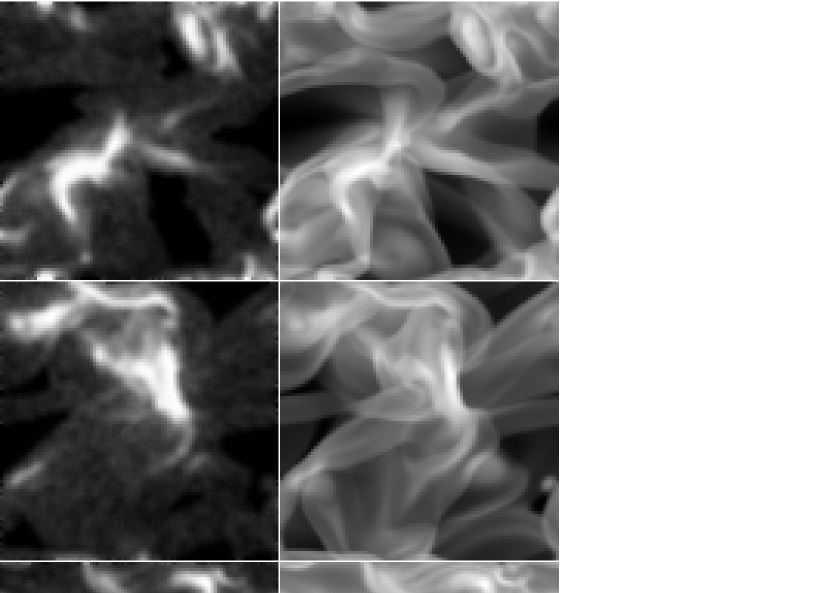
Figure 1: 2-D slices of excitation temperature of ¹³CO, J=1$\rightarrow$0 (left hand side panels), and of the logarithm of the gas density (right hand side panels). The excitation temperature is larger in regions of larger density.

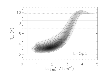
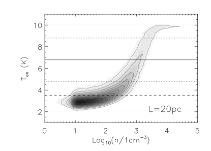
Figure 2: Scatter plot of excitation temperature of ¹³CO, J=1$\rightarrow$0, versus the logarithm of the gas density, in 5pc (left) and 20pc (right) cloud models. The dashed horizontal line marks the mean excitation temperature. The continuous horizontal line marks instead the mean excitation temperature estimated in the LTE calculations to determine the LTE column density N₁ (the dotted lines illustrate the $1-\sigma$ values).

Over most of the calculated volume, the ¹³CO rotational transitions are sub-thermally excited in our artificial clouds. The excitation temperature, $T_{ex}$, is higher in regions of larger gas density. Fig. 1 shows three slices of the 3-D datacubes illustrating typical images of $T_{ex}$ of the J=1$\rightarrow$0 ¹³CO and gas density in the 5 pc cloud model. As expected, $T_{ex}$ correlates with gas density. The distribution of $T_{ex}$ has a smaller dynamic range than the density distribution. The intensity scale in the density map is proportional to the logarithm of the density in order to compress the contrast. Fig. 2 shows scatter plots of $T_{ex}$ versus logarithmic gas density, $Log(n)$. The horizontal dashed line represents the mean excitation temperature $<T_{ex}>$. $<T_{ex}>\approx 4K$ in both cloud models. However, the 20 pc models are a bit ‘colder’ because they have larger regions of very low density gas than the 5 pc models (see Padoan et al. 1997a). The J=1$\rightarrow$0 transition of ¹³CO is therefore strongly sub-thermally excited.

In the following section we estimate the LTE column density for these models. We estimate the excitation temperature from the peak temperature of the J=1$\rightarrow$0 transition of ¹²CO, at every spectrum in the 2–D grids, adopting the abundance ratio [¹²CO]/[¹³CO]=50. The mean value of that temperature is plotted in Fig. 2 as a continuous horizontal line. It is apparent that the estimated value of $T_{ex}$ is about twice as large as the correct one.

3 The LTE and True Column Density

The J=1$\rightarrow$0 transitions of ¹³CO and ¹²CO can be used to estimate the column density of ¹³CO, under the assumption of local thermodynamic equilibrium (LTE). Different authors made use of different approximations, when performing the LTE calculations to estimate column densities from observational data. Therefore we will determine LTE column densities from our models in several different ways to reproduce the various methods presented in the literature. We briefly summarize the formulae that are used in the LTE calculations (eg Dickman 1978; Harjunpää & Mattila 1996) and we then add some simplyfing assumptions.

The two basic assumptions are: (1) The excitation temperature is uniform along the line of sight. (2) The J=1$\rightarrow$0 excitation temperature of ¹³CO and ¹²CO are the same. The excitation temperature, $T_{ex}$, is estimated from the formula:

$$T_{R}=[J(T_{ex})-J(T_{bg})](1-e^{-\tau})$$ (1)

where $T_{bg}=2.7K$ is the background temperature, $\tau$ is the optical depth, $T_{R}$ is the radiation temperature, and the function $J(T)$ is:

$$J(T)=\frac{T_{0}}{exp(T_{0}/T)-1}$$ (2)

where $T_{0}=h\nu_{10}/k$ and $\nu_{10}$ is the frequency of the transition J=1$\rightarrow$0 of ¹³CO. $T_{ex}$ is estimated from the formula (1), where the peak radiation temperature of the J=1$\rightarrow$0 transitions of ¹²CO is used for $T_{R}$, and the same transition is assumed to be optically thick ($\tau\gg 1$). Then equation (1) can be used again, with the estimated value of $T_{ex}$, to determine $\tau$ in each channel, $\tau_{ch}$. The column density of ¹³CO in the ground state, $N_{0}$, is given by:

$$N_{0}=6.39\times 10^{14}\frac{\sum\tau_{ch}\Delta v}{1-e^{-T_{0}/T_{ex}}}cm^{-2}$$ (3)

where $\Delta v$ is the channel width in km s^-1. To obtain the total column density of ¹³CO, $N_{0}$ must be multiplied by the partition function $Q$:

$$N_{1}=N_{0}\times Q=N_{0}\times\sum_{J=0}^{J_{max}}(2J+1)exp\left[\frac{-h\nu_{10}J(J+1)}{2kT_{ex}}\right]$$ (4)

To use equation (4), it is usually assumed that the same $T_{ex}$ is valid for all rotational states of the molecule. The formulae are taken from Harjunpää & Mattila (1996), and we call $N_{1}$ the LTE column density estimated in this way. The optically thin limit ($\tau\ll 1$) is sometimes adopted (eg Park, Hong & Minh 1996), which corresponds to the approximation: $(1-e^{-\tau})\approx\tau$. We call $N_{2}$ the LTE column density estimated under this assumption. Another frequently adopted simplification (eg. Dickman 1978; Park, Hong & Minh 1996) is the following approximation to the partition function:

$$Q\approx 2T_{ex}/T_{0}$$ (5)

(Penzias, Jefferts & Wilson 1971). We call $N_{3}$ the LTE column density estimated like $N_{1}$, but with the approximation (5). In some work (eg Dickman 1978), equation (3) is not evaluated as the sum of $\tau_{ch}\Delta v$ over all channels, but rather using the line center optical depth multiplied by the line full width at half maximum (FWHM). We call this case $N_{4}$, where the partition function is also approximated with the formula (5). Finally, $N_{5}$ is calculated as $N_{4}$, but the FWHM and the peak temperature are that of a Gaussian fit to the line profile.

All results are summarized in Table 1, where the LTE column densities $N_{i}$ are compared with the true column density $N$, that is the ¹³CO column density of the model clouds. The value of $<N_{i}/N>$ illustrates the typical error made with the LTE approximation. On the average, the most detailed LTE calculations yield a value of $N_{1}$ that is about 65% of the true column density in the 5 pc cloud model, and 40% of $N$ in the larger scale 20 pc cloud. LTE column densities estimated with additional approximations underestimate the true column densities even more with the worst case being the optically thin approximation, $N_{2}$, although the J=1$\rightarrow$0 transitions of ¹³CO is optically thin in most of the map. The value of $<N_{i}>/<N>$ is an estimator of the ratio of total estimated mass and real total mass of the cloud. The best case, $N_{1}$, yields 50% and 72% of the total mass of 20 pc and 5 pc models respectively; the worst case, $N_{2}$, yields 37% and 56% of the total mass for the same models. The estimated mean excitation temperature, $<T_{ex}>$, is lower than the kinetic temperature ($T_{K}=10K$), but higher than the true mean excitation temperature of the model clouds (cf Fig. 2). In Fig. 3 the probability distributions of $N_{1}/N$ are plotted for both scales.

In Fig. 4, the value of $<N_{1}>$ is compared with the LTE column density estimated in the same way as $N_{1}$, but assuming a given constant $T_{ex}$ of 4, 6, 8, and 10 K. If very low $T_{ex}$ are adopted, the LTE column density can grow to the point of overestimating the true column density (cf Harjunpää & Mattila 1996, Fig. 2). If instead, the value adopted for the constant $T_{ex}$ is close to the value of $<T_{ex}>$ estimated with the peak temperature of ¹²CO, the constant temperature column densities underestimate $N$ more than $N_{1}$ does. Moreover, the scatter around the estimated mean column density is always larger than for $N_{1}$.

4 Theoretical Calibration of ¹³CO LTE Column Density

Fig. 5 and Fig. 6 are log-log plots of $N_{1}$ versus the true column density $N$. Our models span three orders of magnitude in column density, a much larger range than can be sampled by observations when estimating gas column density using stellar extinction determinations (eg. Encrenaz, Falgarone & Lucas 1975; Tucker et al. 1976; Dickman 1978; Dickman & Herbst 1990; Lee, Snell & Dickman 1991; Lada et al. 1994; Harjunpää & Mattila 1996). As discussed in the introduction, our cloud models have been shown to be consistent with the known properties of MCs. Therefore, we use these models to determine the scale factor $f$ that can be used to convert LTE based column density estimates to a more precise estimate of the true column density. Unfortunately it is rather difficult to fit the relations $N-N_{i}$ with simple mathematical functions. Instead, we plot the calibration factors, $f(N_{i})=N/N_{i}$, for $N_{1}$, $N_{2}$, and $N_{4}$, in Fig. 7. When the LTE column density of ¹³CO is estimated from observational spectra, it should be multiplied by the calibration factor $f(N_{i})$. The LTE column densities perform better at larger density, apart from $N_{2}$ that is good only in the optical thin limit. The often used and simplest LTE estimate, $N_{4}$, is rather good at large density, but it is up to 7 times smaller than the true column density, at low densities.

5 Discussion

Several authors have produced synthetic molecular spectra using simple models for the structure and kinematics of MCs (eg Zuckerman & Evans 1974; Leung & Liszt 1976; Baker 1976; Dickman 1978; Martin, Hills & Sanders 1984; Kwan & Sanders 1986; Albrecht & Kegel 1987; Tauber & Goldsmith 1990; Tauber, Goldsmith & Dickman 1991; Wolfire, Hollenbach & Tielens 1993; Robert & Pagani 1993; Park & Hong 1995; Park, Hong & Minh 1996; Juvela 1997). Leung & Liszt (1976) used a single micro-turbulent cloud and Dickman (1978) a collapsing spherical cloud. Models of many clumps moving at random velocities larger than their intrinsic line-width (macro-turbulence) were used by Zuckerman & Evans (1974) and by Baker (1976). Macro-turbulence was recognized to be necessary to obtain centrally peaked CO line profiles. Macro-turbulent clumpy models include the use of different velocity and clustering laws (eg Kwan & Sanders 1986), increasing clump filling factor towards the center of the cloud (eg Tauber et al. 1991), variations of correlation length in the clump distribution (Albrecht & Kegel 1987), a description of chemical reactions and heating (eg Wolfire et al. 1993), a low density warmer inter-clump medium (Park et al. 1996), density fields generated with fractal models or structure tree statistics (Juvela 1997).

Although clumpy models have being useful to study the properties of MCs, they can only provide a schematic representation of the structure and kinematics of MCs, since their velocity and density fields are not solutions of the fluid equations. MCs are highly dynamical objects with a continuous range of gas density values and therefore a fluid description is appropriate and necessary. Stenholm & Pudritz (1993) and Falgarone et al. (1994) produced molecular spectra from fluid models of clouds. Stenholm & Pudritz (1993) did not solve the MHD equations, but rather used a sticky particles code with an imposed spectrum of Alfvén waves (Carlberg & Pudritz 1990). They computed molecular spectra under the simple assumption of LTE. Falgarone et al. (1994) did not solve the radiative transfer equations, but simply calculated density weighted radial velocity profiles. They used a very high resolution turbulence simulation (Porter, Pouquet & Woodward 1994), but with a low Mach number ($\leq 1.1$) and without magnetic fields. Though these cloud models are solutions of the fluid equations, they are not a realistic representation of the physical conditions in MCs, because of the low Mach numbers and of the low density contrasts.

In the present work we make use of highly supersonic MHD turbulence simulations where the density fields span a continuous range of values covering about six orders of magnitude. We perform the radiative transfer calculations with a non-LTE Monte Carlo code, producing high resolution molecular maps (90$\times$90 spectra) for different molecular transitions. We have already shown in other papers that our cloud models are excellent description of the observed physical conditions in MCs (Padoan, Jones & Nordlund 1997; Padoan & Nordlund 1997; Padoan et al. 1997a; Padoan et al. 1997b).

Our main result is that the LTE ¹³CO column density of MCs underestimates the true column density by a factor of 1.3 to 7. Although previous works have shown that the LTE approximations are good (eg. Dickman 1978; Park, Hong & Minh 1996), these authors found that in regions of low density, the LTE column density is underestimated. Our results are consistent with previous studies. In our more realistic cloud models the density has a continuous distribution and a large fraction of the volume is at very low densities where conditions are far from LTE. As an example, in our models, only 20-30% of the total mass resides in regions where the density is larger than in the clumps modeled by Park et al. (1996). On the other hand, the peak density in our model is larger than in Park et al. (1996) model.

In Fig. 8 we show that three basic assumptions of the LTE calculations are not correct. The probability distribution functions of $T_{ex}$ of different transitions show that: (1) $T_{ex}$ values are considerably smaller than the kinetic temperature (10 K); (2) $T_{ex}$ of ¹³CO and ¹²CO are quite different; (3) the $T_{ex}$ along a single line of sight is not uniform, but has a broad distribution of values. It is not surprising therefore to find discrepancies between LTE column densities and true column densities.

In this work we have treated the small scale (5 pc) and large scale (20 pc) simulations separately. The distinction is important, because the volume filling factor of dense regions grows with decreasing scale. The peak density in a simulation is independent of simulation scale but the mean density is lower in the larger simulations where the density contrast is larger. Larger scales have stronger turbulent motions that cause a larger density contrast compared with smaller scales. Therefore, the calibration of LTE column densities, using a realistic cloud model, requires consideration of the length scales involved.

Observations have demonstrated that external radiation fields tend to make cloud exteriors warmer than their interiors (cf. Castets et al 1990). The ¹²CO cloud ‘photosphere’ (where the line optical depth reaches unity) tends to lie in a warmer region than the portion of the cloud where the ¹³CO emission is produced. Thus, estimates of T_ex based on ¹²CO tend to overestimate its true value. This leads to an additional underestimation of the column density.

Both the MHD and radiative transfer calculations adopted a constant temperature. Heating and cooling processes are assumed to exactly balance at one specific temperature. If the thermal balance and temperature were computed self-consistently, the results of the present calculations could be slightly altered.

Figure 3: Probability distributions of the best LTE column density estimate divided by the true column density, $N_{1}/N$.

Figure 4: Estimated LTE column densities, using the same assumptions as in N₁, but with a constant T_ex. The bars represent the $1-\sigma$ dispersion around $<N_{LTE}/N_{TRUE}>$. The diamond symbol marks the value of $<N_{1}/N>$ and the mean excitation temperature, $<T_{ex}>$, estimated to determine N₁.

Figure 5: LTE column density of ¹³CO, versus the true column density, for 5pc cloud models. LTE always underestimate the true column density.

Figure 6: LTE column density of ¹³CO, versus the true column density, for 20pc cloud models. LTE always underestimate the true column density.

Figure 7: Ratios of true and LTE column density, versus LTE column density.

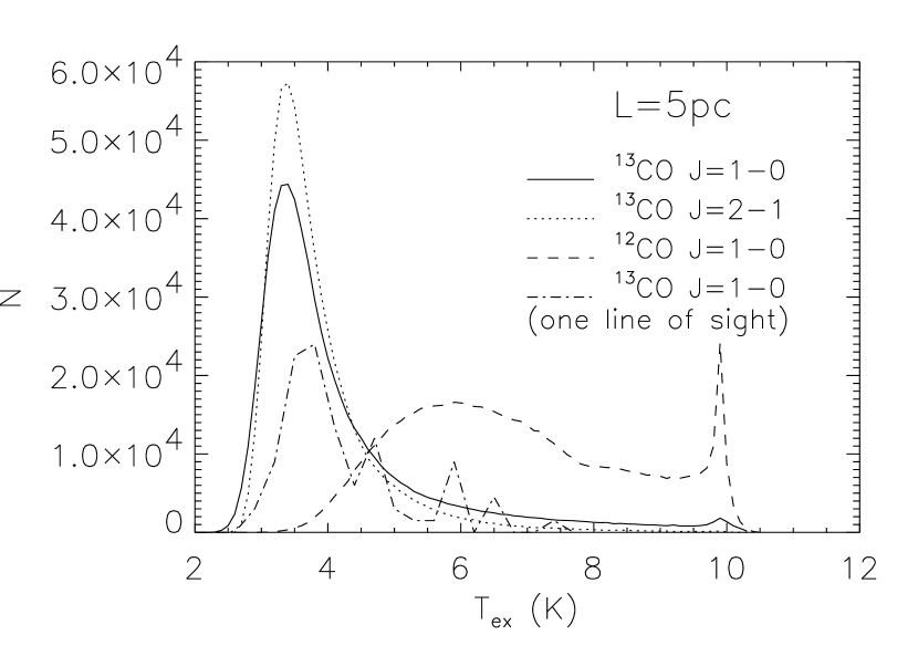
Figure 8: Probability distribution functions for $T_{ex}$ of different transitions. The dashed dotted line is the histogram for a single line of sight (multiplied by a factor 1500). $T_{ex}$ of the two transitions of ¹³CO have rather similar distributions, but the distribution of $T_{ex}$ of ¹²CO is very different, at variance with one of the basic assumptions of the LTE calculations. Moreover the $T_{ex}$ along a single line of sight is not uniform (as assumed in the LTE calculations), but has a broad distribution.

L=20pc; $<T_{ex}>6.8\pm 2.0K$	N1	N2	N3	N4	N5
$<N_{i}/N>$	0.40 $\pm$0.18	0.35 $\pm$0.13	0.35 $\pm$0.17	0.35 $\pm$0.20	0.34 $\pm$0.19
$<N_{i}>/<N>$	0.50	0.37	0.45	0.49	0.46
L=5pc; $<T_{ex}>8.4\pm 1.4K$	N1	N2	N3	N4	N5
$<N_{i}/N>$	0.65 $\pm$0.16	0.56 $\pm$0.11	0.59 $\pm$0.15	0.60 $\pm$0.21	0.59 $\pm$0.19
$<N_{i}>/<N>$	0.72	0.56	0.65	0.71	0.69

Table 1: Ratios of different LTE estimations of column density (N_i) and real column density (N), for ¹³CO, J=1$\rightarrow$0. See the text for the definition of the N_i.

References

- (1) Albrecht, M. A. & Kegel, W. H. 1987, A&A, 176, 317
- (2) Backer, P. L. 1976, A&A, 50,327
- (3) Bohlin, R. C., Savage, B. D. & Drake, J. F. 1978, ApJ, 224, 132
- (4) Carlberg, R. G. & Pudritz, R. E. 1990, MNRAS, 247, 353
- (5) Castets, A., Duvert, G., Dutrey, A., Bally, J., Langer, W. D., & Wilson, R. W. 1990, A&A, 234, 469
- (6) Dickman, R. L. 1978, ApJS, 37, 407
- (7) Dickman, R. L. & Herbst, W. 1990, ApJ, 357, 531
- (8) Encrenaz, P. J., Falgarone, E. & Lucas, R. 1975, A&A, 44, 73
- (9) Falgarone, E., Lis, D. C., Phillips, T. G., Pouquet, A., Porter, D. H. & Woodward, P. R. 1994, ApJ, 436, 728
- (10) Harjunpää, P. & Mattila, K. 1996, A&A, 305, 920
- (11) Kwan, J. & Sanders, D. B. 1986, ApJ, 309, 783
- (12) Jenkins, E. B. & Savage, D. B. 1974, ApJ, 187, 243
- (13) Juvela M., 1997, A&A (in press)
- (14) Lada, C. J., Lada, E. A., Clemens, D. P., & Bally, J. 1994, ApJ, 429, 694
- (15) Lee, Y., Snell, R. L. & Dickman, R. L. 1991, ApJ, 379, 639
- (16) Leung, C. M. & Liszt, H. S. 1976, ApJ, 208, 732
- (17) Lilley, A. E. 1955, ApJ, 121, 559
- (18) Martin, H. M., Hills, R. E. & Sanders, D. B. 1984, MNRAS 208, 35
- (19) Padoan, P., Jones, B. J. T. & Nordlund, Å. 1997, ApJ, 474, 730
- (20) Padoan, P. & Nordlund, Å. 1997, Apj, submitted
- (21) Padoan, P., Juvela, M., Bally, J. & Nordlund, Å. 1997a, Apj, submitted
- (22) Padoan, P., Juvela, M., Zweibel, E. & Nordlund, Å. 1997b, in preparation
- (23) Park, Y. S., Hong, S. S. & Minh, Y. C. 1996, A&A, 312, 981
- (24) Robert, C. & Pagani, L. 1993, A&A, 271, 282
- (25) Stenholm, L. G. & Pudritz, R. E. 1993, ApJ, 416, 218
- (26) Tauber, J. A. & Goldsmith, P. F. 1990, ApJ, 356, L63
- (27) Tauber, J. A., Goldsmith, P. F. & Dickman, R. L. 1991, ApJ, 375, 635
- (28) Tucker, K. D., Dickman, R. L., Encrenaz, P. J. & Kutner, M. L. 1976, ApJ, 210, 679
- (29) Wolfire, M. G., Hollenbach, D. & Tielens, A. G. G. M. 1993, ApJ, 402, 195
- (30) Zuckerman, B. & Evans, N. J. 1974, ApJ, 192, L149