Energy Input and Mass Redistribution by Supernovae in the Interstellar Medium

Abstract

We present the results of numerical studies of supernova remnant evolution and their effects on galactic and globular cluster evolution. We show that parameters such as the density and the metallicity of the environment significantly influence the evolution of the remnant, and thus change its effects on the global environment (e.g., globular clusters, galaxies) as a source of thermal and kinetic energy.

We conducted our studies using a one-dimensional hydrodynamics code, in which we implemented a metallicity dependent cooling function.

Global time-dependent quantities such as the total kinetic and thermal energies and the radial extent are calculated for a grid of parameter sets. The quantities calculated are the total energy, the kinetic energy, the thermal energy, the radial extent, and the mass. We distinguished between the hot, rarefied bubble and the cold, dense shell, as those two phases are distinct in their roles in a gas-stellar system.

We also present power-law fits to those quantities as a function of environmental parameters after the extensive cooling has ceased. The power-law fits enable simple incorporation of improved supernova energy input and matter redistribution (including the effect of the local conditions) in galactic/globular cluster models.

Our results for the energetics of supernova remnants in the late stages of their expansion give total energies ranging from $\approx 9\times 10^{49}$ to $\approx 3\times 10^{50}$ ergs, with a typical case being $\approx$ 10⁵⁰ erg, depending on the surrounding environment. About $8.5\times 10^{49}$ erg of this energy can be found in the form of kinetic energy.

Supernovae play an important role in the evolution of the interstellar medium and galaxies as a whole, providing mechanisms for kinetic energy input and for phase transitions of the interstellar medium. However, we have found that the total energy input per supernova is about one order of magnitude smaller than the initial explosion energy.

1 INTRODUCTION

The role of supernovae (SNe) as sources of matter and energy to the interstellar medium (ISM) has been confirmed by numerous observations and theoretical studies. It is believed that supernova explosions are the source of the hot galactic and halo gas that is seen in X-rays. SNe are by far the major source of the heavy elements (Woosley & Weaver 1986), and the study of metal abundances has proven to be very useful in tracing the history of our Galaxy and other galaxies. SNe are also the major source of the kinetic energy of interstellar clouds. Aboott (1982) estimated that the supernova energy input is larger by about a factor of five than the combined input from O, B, A, supergiant, and Wolf-Rayet stars, assuming Type I and Type II SN energies of $5\times 10^{50}{\rm ergs}$ and $10^{51}{\rm ergs}$, respectively. Such energy sources influence the subsequent star formation in the ISM, which in turn changes the SN rate and the resulting energy input. The interactions between the various physical processes in the ISM complicate studies of the ISM. In particular, since supernovae are the major source of energy to the ISM, a proper treatment of supernovae in the modeling of the dynamical evolution of galaxies or globular clusters is essential.

There have been many studies of the interactions of supernova remnants (SNRs) with the ISM and the late stages of remnant evolution. Over the last decades, much progress has been made in understanding the behavior and the characteristics of SNRs. These studies include analytical and numerical models of various stages of the remnant evolution. Chevalier and coworkers considered SNRs in a spherically symmetric medium (Chevalier 1974, 1984) and a plane-stratified medium (Chevalier & Gardner 1974). More recently, they extended their work to study the instabilities due to radiative cooling (Chevalier & Blondin 1995). Those studies tended to focus on the SNR evolution itself in an attempt to explain the observations of SNR of various ages.

Other studies focused on the interactions between the SNRs and the ISM. Cox and Smith (1974) suggested that SN explosions could create a hot gas phase in the ISM. McKee & Ostriker (1977) proposed that the interstellar medium consists of three phases: a cold neutral medium, a warm ionized medium, and a hot ionized medium. Slavin & Cox followed these studies with detailed predictions of column densities of highly ionized elements, such as O 6, Si 4, and C 4 (Slavin & Cox 1992), and the porosity factor (Slavin & Cox 1993) of the solar neighborhood. Cioffi, McKee, & Bertschinger (1988) (hereafter, CMB) studied the evolution of a SNR using a one-dimensional numerical hydrodynamical model, which included the effects of cooling by radiation. The results were later applied to model the ISM in a galactic disk (Cioffi & Shull 1991). However, these studies were carried out only for the case of a typical present-day interstellar environment with solar metallicity (or, at best, of an environment of relatively comparable properties). The studies to date have been mainly intended to provide an understanding of the observations of the present-day SNRs and ISM, and thus the results were not extended for applications to the modeling of formation and early evolution of stellar systems. An example of the exception is the work by Hellsten & Sommer-Larson (1995), who performed numerical simulations and an analytical study to calculate the mass fraction of hot gas in supernova remnants for a range of ISM densities and for a few choices of metallicities. The result, however, was limited to the fraction of hot gas, and provided no clear method for its application. Therefore, a systematic study of the effect of SN explosions in various environments that exist in the course of galactic evolution has not been carried out. As a result, no realistic prescription for SN energy dispensation is yet available to researchers interested in proper modeling of galaxies.

As more sophisticated models of galaxies and other stellar systems have been developed, the need has increased for more accurate data which describe the behavior of SNe in various environments. Due to the lack of such information, simplifying assumptions have been made in models which involve supernova heating and kinetic energy input. A common method of incorporating SNe energy input is simply to assume a typical SN explosion energy of about $10^{51}{\rm ergs}$ (Leitherer, Robert, & Drissen 1992, Burkert, Hensler, & Truran 1992). Due to the uncertainty as to how efficiently the explosion energy is transferred to the ISM, some studies introduce a parameter, the “efficiency”, which measures how much of this explosion energy becomes available to the ISM. The uncertainty in our knowledge of the magnitude of this efficiency is reflected in the wide range of assumed values: from 1% for kinetic energy (e.g., Padoan, Jimenez, & Jones 1997) up to 100% (e.g., Burkert et al. 1992; Theis, Burkert, & Hensler 1992; Rosen and Bregman 1995). In some cases, the values of efficiency are determined by fits to the observation. There are also studies in which the supernova explosion energy of $10^{51}{\rm ergs}$ is put purely into the thermal energy (Katz 1992, Steinmetz & Müller 1995). They concluded that input in thermal energy is easily radiated away, and thus has insignificant effect in their models. Navarro & White (1993) found a strong dependence of the evolution of galaxies on the fraction, $f_{v}$, of energy input that is provided in the kinetic form. Cole et. al. (1994) concluded that $f_{v}$ of about 10% to 20% provided a good fit to observational data (such as the galaxy luminosity functions, galaxy colors, the Tully-Fisher relation, faint galaxy number counts, and the redshift distribution). To limit the uncertainties in the quantities and the fractions of energies that the supernovae provide, it is important to determine the input from a basic physical approach.

SNRs are also known to produce dense, cold environments, or clouds, in the shell during their late evolution. This provides an important site for star formation. Although such effects have been studied in terms of “enhanced star formation rate” (Ikeuchi & Habe 1984), they have not been examined consistently with respect to either the energy input or to the nature of the environment.

In this paper, we present our approach to this problem, as well as some selected results from the grid of models, which provides information about the global characteristics of SNRs in various environments. We will present the results of numerical simulations for a range of conditions relevant to the entire period of galactic formation and evolution, including the halo formation period, as well as globular cluster formation.

This paper is organized as follows. In §2, we discuss our numerical simulations in some detail. In §3, we present the results from our calculations, focusing on the physical processes involved. In §4, we present a set of power-law fits to our numerical results of quantities which characterize the effects of SNe in various ISM environments. We then discuss, in §5, some of the assumptions we have made in the calculations, and possible implications of our results for dynamical and chemical evolution of galaxies and globular clusters. Our conclusions are presented in §6.

2 NUMERICAL SIMULATIONS

2.1 Assumptions and Input Physics

The Lagrangian equations governing the spherically symmetric hydrodynamical system are:

$${1\over\rho}={4\pi\over 3}{\partial r^{3}\over\partial m},$$

$${{\rm d}r\over{\rm d}t}=v,$$

$${{\rm d}v\over{\rm d}t}=-{1\over\rho}{{\partial P}\over{\partial r}}-{Gm(r)\over r^{2}},$$

$${{{\rm d}\varepsilon}\over{{\rm d}t}}={(P+\varepsilon)\over{\rho}}{{\rm d}\rho\over{{\rm d}t}}-n_{e}n_{H}\Lambda(T),$$

$$P=(\gamma-1)*\varepsilon,$$

$$T={\mu m_{H}P\over{k\rho}},$$

where $\varepsilon$ is the energy density, $n_{e}$ and $n_{H}$ are the electron and the hydrogen number densities, respectively, $\Lambda(T)$ is the cooling function, and $m_{H}$ is the mass of hydrogen. Other variables have their standard definitions. These equations are solved using the numerical methods described by Janka, Zwerger, & Mönchmeyer (1993). The boundaries were closed both at the center and at the outer end. Additional zones are added as the shock shell approaches the outer boundary, so that the closed boundary does not affect the evolution.

In this work, we provide an improved measure of the thermal and kinetic energy input of supernovae to their environments for a grid of initial conditions. In particular, we examine the effects of varying the metallicity and the density in the environment. The ranges of initial composition and ambient density are chosen to provide adequate coverage for early and late galactic environments. For the metallicities, mass fractions of metal $Z=0.00$, $0.01$, $0.02(\equiv Z_{\hbox{$\odot$}})$, and $0.04$ are chosen. We consider densities, $\rho_{0}$, ranging from 0.0133 to 13.3 $m_{H}/{\rm cm}^{3}$ (corresponding to $n_{H}$ of $0.01$ to $10.0{\rm cm}^{-3}$ with $Z=0.02$). Wider ranges in both the metallicity and the density are adopted for calculations for the power-law fits (see §4).

The gas is assumed to be composed of 23% helium, $(77-Z\times 100)$% hydrogen and $(Z\times 100)$% metals by mass, and to be monatomic and nonrelativistic, so that $\gamma=5/3$. Each simulation starts with 1800 grid points distributed over 100 pc, with 150 grid points in the innermost region where the supernova explosion energy and the ejecta mass are located initially.

The initial configurations are:

• Outer region (ISM): The density and the metallicity are assumed constant at the chosen values, which are varied between different calculations.

• Inner region (exploding SNR, inner 1.5 pc):

  • 1. Ejecta Mass: 3 $M_{\hbox{$\odot$}}$ are distributed uniformly, in addition to the mass contributed by the ISM in this volume. The results of our calculations are not strongly dependent upon the assumed mass of the supernova ejecta.

    2. Thermal Energy: $6.9\times 10^{49}$ ergs are distributed uniformly over the region.

    3. Kinetic energy: $9.31\times 10^{50}$ ergs are distributed such that the velocity profile is linear (similar to the Sedov solution).

A critical piece of input physics for our study is the cooling functions. We adopt the metallicity dependent cooling functions calculated by Böhringer and Hensler (1989), which assume optically thin gas in thermal equilibrium. This study includes atomic lines of the ten most abundant elements (H, He, C, N, O, Ne, Mg, Si, S, and Fe) in the wavelength range 1.5 Å to 2340 Å. The actual cooling rate is given by $n_{e}n_{H}\Lambda(T)$, where $\Lambda(T)$ is the cooling function, T is the gas temperature, and $n_{e}$ and $n_{H}$ are the number densities of electrons and hydrogen, respectively.

Below the temperature of $10^{4}$ K, the cooling function depends on the trace ionization. We estimate the cooling in this regime from the cooling functions of Dalgarno and McCray (1972), using a normalization consistent with our work. It should be noted that the cooling functions we have adopted in the low temperature regime ignore molecular and neutral atomic processes. This is a possible weakness in this work. However, in order to make our treatment more realistic, a detailed study of radiative processes involving molecules and neutral atoms, including reliable population information for each species, must be obtained first. We have chosen to make conservative estimates of the cooling to provide a lower limit to the energy lost to radiation.

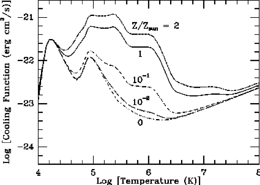
Figure 1: Cooling functions adopted for the calculation for temperatures above $10^{4}$ K from Böhringer & Hensler (1989).

The cooling functions we have adopted in our calculations are shown in Figure 1. Cooling functions simplify the implementation of cooling by collecting the effects of radiation from many atomic species. Only hydrogen and helium contribute to the cooling for the case of primordial galactic matter, and therefore, the coefficient is lower than the case of the solar metallicity. In particular, the metal cooling is very efficient in the temperature range $10^{5}$ K to $10^{7}$ K, and thus even trace amounts of metals dominate in the temperature range. For a solar metallicity environment, the metals dominate the cooling rate by as much as a factor of 10 - 100 in the temperature range $10^{5}-10^{7}$ K.

It should be noted that the various studies adopted different descriptions for the cooling (both in the cooling coefficient and in its normalization; a normalization to $n_{H}^{2}$, rather than to $n_{e}n_{H}$, is more commonly used). For example, CMB adopted a simple description of cooling in which the cooling function is proportional to the powers of the metallicity and the temperature. This enabled them to solve a simplified differential equation analytically for the expansion of a cooling SNR in an environment with metallicities similar to the solar case. However, in the limit of very low metallicity, the solution breaks down, since the dominant cooling is provided by hydrogen and helium, for which a simple power-law cooling function does not apply. For numerical studies, there are various factors which must be considered in calculating cooling functions, such as the composition of the metal component, the radiative transitions to include, and the normalizations (i.e., the cooling rate is proportional to the product, $n_{e}n_{H}$, etc.). We tested our results above $T=10^{4}$ K using a cooling function calculated by Sutherland & Dopita (1993), which is slightly different from that of Böhringer & Hensler(1989), and found good agreement. For the case with solar metallicity and an ambient density of $0.1~{}{\rm hydrogen}/{\rm cm}^{3}$, the comparison between the two results yielded a difference in the total energy of 2.4%, or 4.1$\times 10^{48}$ ergs at the time the total energy settled to approximately a constant value. This indicates that the cooling function above $T=10^{4}$ K is known sufficiently well for the purposes of this study. For temperatures below $10^{4}$ K, we expect the uncertainty to be larger since the calculation of the cooling function in the regime is complicated by molecular cooling.

The metallicity of the gas, used in calculating the metal-dependent cooling, is assumed constant at the ambient medium value. Although there is an enhancement of heavy elements in the region where mixing takes place, it has been determined from 2-D hydrodynamics calculations that this occurs only in the inner region well away from the shock front where most of the cooling takes place (Gaudlitz 1996). The cooling rate in the very low density bubble, where possible enhancement of metals occur, is much smaller than that of the shell, despite the high metallicity. Therefore, the small error in the local cooling rate in the bubble is negligible.

Following CMB, we assume that the gas is fully ionized. The effects of magnetic fields are ignored in the present calculations; we will consider the possible consequences of this assumption in our discussion in §5.

It is recognized that the region behind the shock is under-ionized, due to the fact that the ionization time becomes longer than the local dynamical time. In order to properly treat this effect, time-dependent ionization and recombination must be implemented, instead of simply assuming full ionization. We do not expect that these small modifications to the pressure and to the cooling history will change the global properties of the SNR significantly. It should be kept in mind that a precise treatment of ionization is essential if a model is to be used to predict emission spectra from SNRs, which are sensitive to level populations.

The effects of thermal conduction may be important in the late stages of the SNR evolution. We expect that conduction should indeed modify the temperature profile in the SNR. However, we do not expect a significant change in the cooling itself, since the temperature in the shell (where most cooling takes place) is not affected significantly. Also, it is difficult to quantify the effects of conduction, because turbulent magnetic fields are known to suppress conduction. Since we do not have any information on the magnitude of turbulence or on the strength of the magnetic fields, we have chosen not to include the effects of conduction in this study.

In addition, we ignore the kinetic energy loss due to cosmic-ray radiation. This energy loss is expected to occur at a very early stage of the SNR evolution; therefore, the effect can be taken into account simply by scaling the results with the initial energy.

2.2 Hydrodynamic Code and Test Calculations

We mainly employed an explicit Lagrangian finite-difference scheme, which is second-order accurate in space and in time, in our numerical studies. For treating shock discontinuities, a tensor form of the artificial viscosity (Tscharnuter & Winkler 1979) is used. The code has been tested extensively through standard problems with known solutions, and its performance compared well to a PPM code (Janka, Zwerger, & Mönchmeyer 1993).

The energy loss due to radiation was treated as a source term, which is implemented by an operator-splitting method. The electron abundance was calculated as discussed previously, and was used both in the equation of state and in calculating the cooling rate.

The time steps are limited so that no quantities change by more than 10% within a time step, as well as by the time step constraints arising from the Courant-Friedrichs-Lewy stability condition, the dynamical time, and the cooling time.

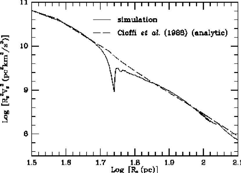
Figure 2: The product, $R_{s}^{2}V_{s}^{3}$, is plotted against $R_{s}$ for the parameter set $n_{H}=0.1/{\rm cm}^{3}$ and $Z=0.02$ (solar metallicity). $R_{s}$ and $V_{s}$ are the radius and velocity of the shock.

As a first test of our calculation, our results are compared to that of CMB for an appropriate parameter set ($n_{H}=0.1/{\rm cm}^{3}$, $Z=0.02$). We found the results to be consistent within the expected difference due to the choice of the cooling functions. An example is given in Figure 2, which should be compared with Figure 8 of CMB. The plotted quantity is $R_{s}^{2}V_{s}^{3}$ vs. $R_{s}$, where $R_{s}$ is the radius at which the shock is located, and $V_{s}$ is the shock velocity. The quantity $R_{s}^{2}V_{s}^{3}$ is closely related to the luminosity, as it is equal to the decrease in kinetic energy, which is approximately ${1\over 2}\dot{M}V_{s}^{2}$. The second term in the expression for the rate of kinetic energy change becomes negligible as the time increases, since it is proportional to $\dot{V}_{s}$, which is a rapidly decreasing function of time. The dotted lines are the analytic solution given in CMB. The analytic solutions in the two plots differ slightly. We have used the following expressions for the radius $R_{s}$ and velocity $V_{s}$ of the shell, as provided by CMB:

$$R_{s}=R_{PDS}{\left({4\over 3}t_{*}-{1\over 3}\right)}^{3/10},$$

$$V_{s}=V_{PDS}{\left({4\over 3}t_{*}-{1\over 3}\right)}^{-7/10},$$

where

$$R_{PDS}=14.0{{E_{51}^{2/7}}\over{n_{H}^{3/7}\zeta^{1/7}}}pc,$$

$$V_{PDS}=413n_{H}^{1/7}{E_{51}^{1/14}}\zeta^{3/14}km/s,$$

$$t_{*}={t\over t_{PDS}},$$

$$t_{PDS}=1.33\times 10^{4}{{E_{51}^{3/14}}\over{\zeta^{5/14}n_{H}^{4/7}}}yr.$$

The subscript PDS indicates the quantities at the onset of the pressure-driven snowplow phase, i.e., at $t=t_{PDS}$. $n_{H}$ is the ambient hydrogen density which was set to $0.1/{\rm cm}^{3}$ in both calculations. $\zeta$ is the metallicity parameter, $Z/Z_{\hbox{$\odot$}}$, which was set to 1. $E_{51}$ is the initial explosion energy in $10^{51}$ ergs. CMB used a slightly different value of $R_{PDS}$ (36.8 pc, as opposed to 37.6 pc as given by the equation for $n_{H}=0.1/{\rm cm}^{3}$), corresponding possibly to a slightly different value of $n_{H}$, $0.105/{\rm cm}^{3}$. It is clear that our results closely follow their analytic solution and numerical solution. The slight differences are most likely due to the differences in the adopted cooling functions.

The extreme thinness of the shell at the time the cooling is most efficient can cause numerical problems. Special care was given to the region at and around the thin shell to make sure that our calculation were well resolved at all times. This was achieved by a combination of visual inspections of the shell region and by running test cases with higher and lower resolutions.

3 RESULTS OF SNR EVOLUTION

The numerical results of our calculations of supernova remnant evolution are presented in this section. We calculate the total energies, the kinetic energies, and the thermal energies of the SNR models, differentiating shell energies from bubble energies. We also calculate the radial extent of SNR, and the SNR and the shell masses as functions of time. These quantities provide the information necessary for proper dispensation of energies and matter in stellar system formation/evolution models. The boundaries of the shell were determined by over-density of 10%, as compared to the unshocked medium. Test calculations were performed with another selection criterion, which separates the hot bubble and the cold shell at the temperature of $10^{5}$ K, and we found no significant differences.

We are interested in metallicities ranging down to the low values characteristic of halo environments (see e.g. the reviews by Wheeler, Sneden, & Truran (1989)). Observations have identified stars with metallicities as low as $[{\rm Fe}/{\rm H}]=-3$ to $-4$ (McWilliam, Preston, Sneden, & Searle 1995, Ryan, Norris, & Beers 1996). In addition, observations of QSO absorption systems indicate metallicities as low as $[{\rm Fe}/{\rm H}]=-2$ to $-2.5$, which may correspond to the metallicities of protogalactic environments (Cowie, Songaila, Kim, & Hu 1995; Rauch, Haehnelt, & Steinmetz 1997; Timmes, Lauroesch, & Truran 1995; Lauroesch, Truran, Welty, & York 1996; Lu, Sargent, Barlow, Churchill, & Vogt 1996; Pettini, King, Smith, & Hunstead 1997). We have therefore included $\log[Z/Z_{\hbox{$\odot$}}]$ down to $-3$. The results from the lowest metallicity case is applicable also for a zero metallicity environment, as explained later. The density ranges are taken from the cold cloud like conditions of $n_{H}=10^{3}/{\rm cm}^{3}$ to a very hot rarefied gas of $n_{H}=10^{-3}/{\rm cm}^{3}$. These metallicity and density ranges should suffice for the application of our results to diverse star-forming environments.

3.1 Behavior of Global Quantities and Details of Remnant Structure and Evolution

We will first provide an overview of the behavior of the global quantities such as the total energy and the radius of the SNR in various phases of SNR evolution. We will then present the structural information which illustrates the physical mechanisms governing the behavior of the SNR in those phases. For this purpose, we will take representative snapshots from the phases of the remnant evolution typical of the present-day interstellar environment: $Z=0.02$, $n_{H}=0.1/{\rm cm}^{3}$.

The ejecta-dominated phase, a very early phase in SNR evolution where the ejecta mass dominates the swept-up ambient matter, is not studied here since the calculations do not properly simulate it. During this phase, the SN ejecta expand into space much like expansion in a vacuum, since the surrounding matter does not influence the system significantly. Our calculation does not provide realistic information on this phase, since the results at the time corresponding to the end of the phase are still influenced by the initial conditions, and in some high density cases, the calculations are started at conditions corresponding to those occurring after this phase has effectively ended. Since our focus is on the effect of SNRs on the surrounding ISM, the details of the ejecta-dominated phase (when the influence of the SNR is still confined to a small region of the ISM) are not of direct interest for this paper. The phase has been well studied in order to explain X-ray emissions from young SNe, and we refer the readers to previous studies (Hamilton & Sarazin 1984; McKee & Truelove 1995 (this paper also contains discussion of the Sedov-Taylor phase and of the transition between the two); Spicer, Clark, & Maran 1990; Kazhdan & Murzina 1992). Our results properly represent the SNRs starting at the adiabatic expansion phase. We will now describe our results and the physical processes which dictate the observed behaviors.

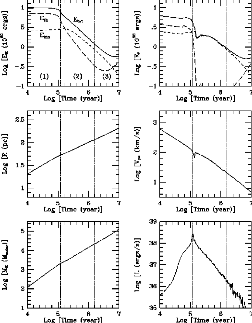
Figure 3: Total energy, kinetic energy, and thermal energy of the SNR ($E_{Rtot}$ (solid line), $E_{Rkin}$ (dashed line), and $E_{Rth}$ (long dashed line), respectively) and of the shell ($E_{Stot}$ (solid), $E_{Skin}$ (dash), and $E_{Sth}$ (long dash), respectively) vs. time, illustrating the evolution of the SNR. The ambient density is taken to be $\rho_{0}=0.133m_{H}/{\rm cm}^{3}$, and the metallicity is set to $Z_{\hbox{$\odot$}}$. In addition, the radius $R$ and the mass $M_{R}$ of the SNR, post-shock fluid velocity $V_{ps}$, and the luminosity $L$ (or the energy loss rate) of the SNR are plotted. The vertical dotted lines indicate the approximate phase boundaries (see text).

We will divide the evolution of a SNR (subsequent to the ejecta-dominated phase) into three phases, according to the governing physical processes: 1) the adiabatic (or Sedov-Taylor) phase (Sedov 1959; Taylor 1950), 2) the cooling (radiative shock, or pressure-driven snowplow) phase (Cox 1972; Chevalier 1974), and 3) the post-cooling phase. Evolution of SNRs beyond the post-cooling phase is not a focus of this paper; therefore, we will only mention the possible fate of SNR in §3.1.3 briefly. These evolutionary phases are roughly indicated by the numbers in Figure 3, which shows various global quantities as functions of time. The total energy, the kinetic energy, and the thermal energy of the SNR and of the shell, the radius $R$ and mass $M_{R}$ of the SNR, the post-shock fluid velocity, and the luminosity (or the energy loss rate) $L$ of the SNR, are shown. The boundaries between the phases are noted on each plot.

The curves describing the changes in the energetics of the SNR allow us to distinguish an early phase where cooling does not affect the structure (i.e. cooling is still negligible and the shell is still thick), and a phase where cooling has become important and a thin shell has formed. This can be seen in the behavior of the total energy plotted in Figure 3, as a flat plateau at early times, followed by a rapid energy decrease. The third phase, the post-cooling phase, is seen as a flattening of the total energy curve after the rapid decrease. These phases are briefly examined below, along with the structural information.

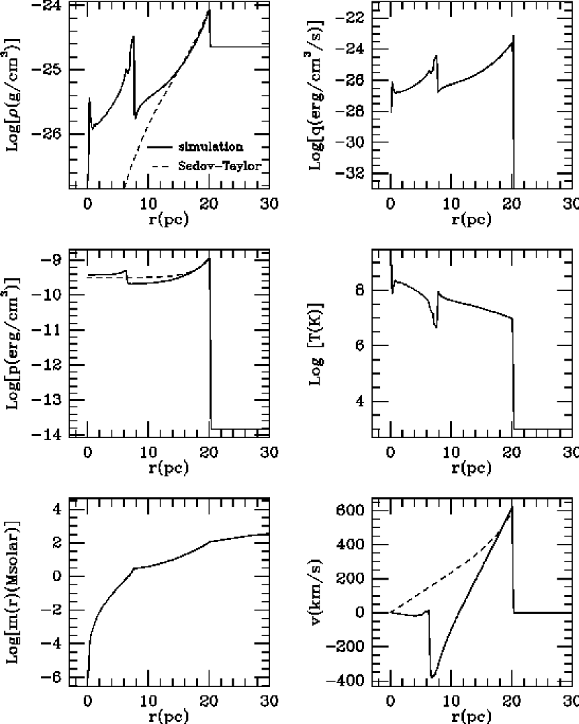
Figure 4: Density $\rho$, pressure $p$, cumulative mass $m(r)$, cooling rate per unit volume $q$, temperature $T$, and fluid velocity $V$ as a function of radius $r$, at time $t=9810$ yr. The dashed lines represent Sedov-Taylor solution. The ambient density is taken to be $\rho_{0}=0.133m_{H}/{\rm cm}^{3}$, and the metallicity is set to $Z_{\hbox{$\odot$}}$.

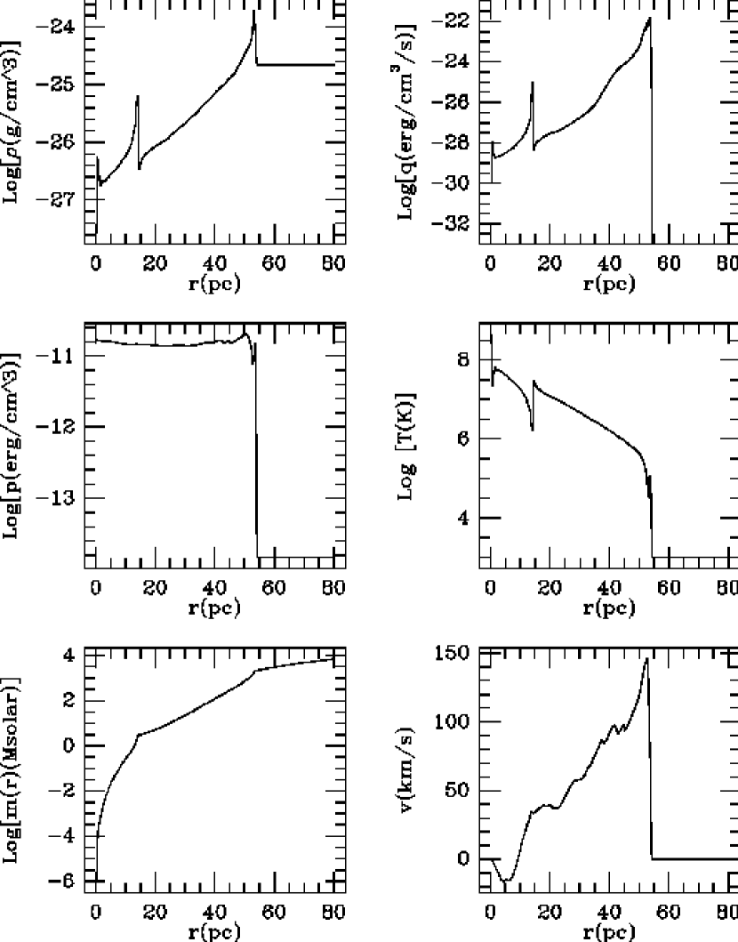
Figure 5: Density $\rho$, pressure $p$, cumulative mass $m(r)$, cooling rate per unit volume $q$, temperature $T$, and fluid velocity $V$ as a function of radius $r$, at time $t=1.27\times 10^{5}$ yr. The ambient density is taken to be $\rho_{0}=0.133m_{H}/{\rm cm}^{3}$, and the metallicity is set to $Z_{\hbox{$\odot$}}$.

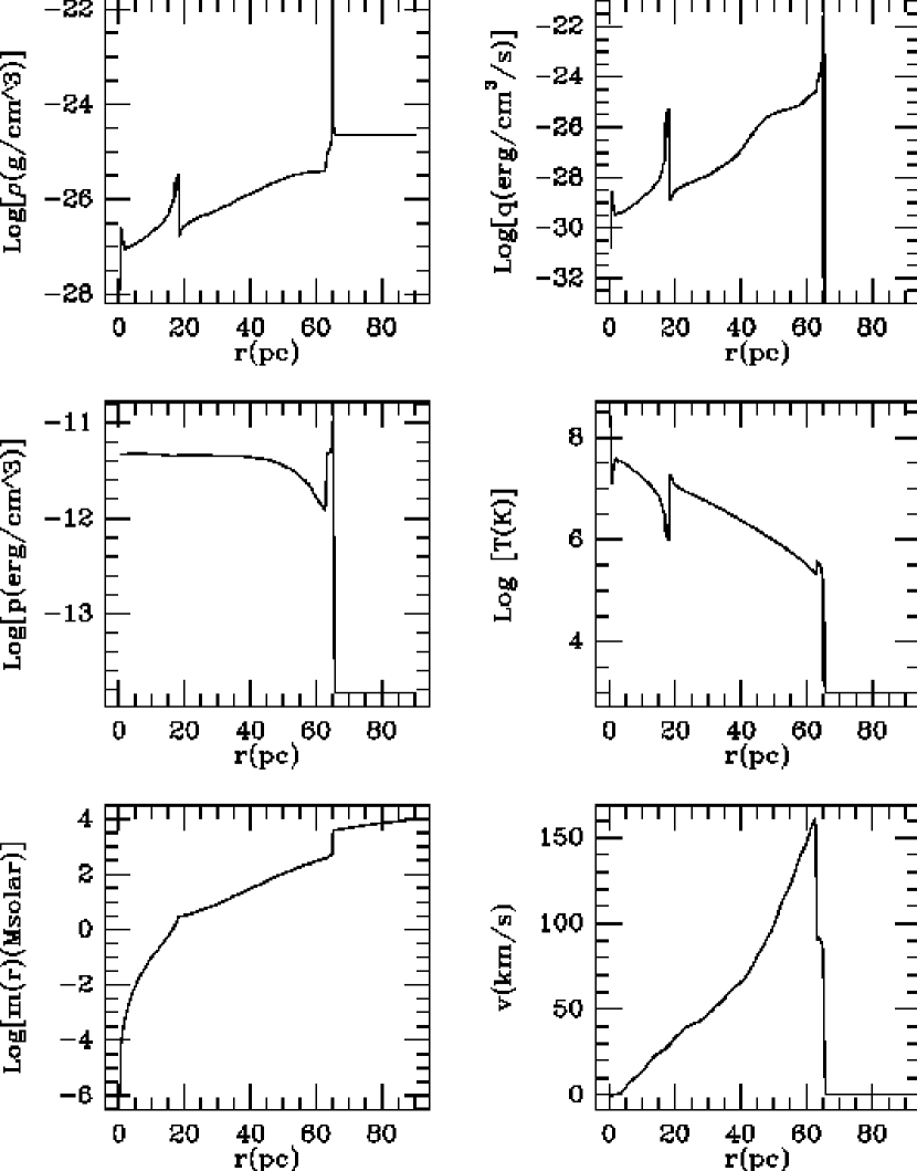
Figure 6: Same as Fig. 5 at $t=2.54\times 10^{5}$ yr.

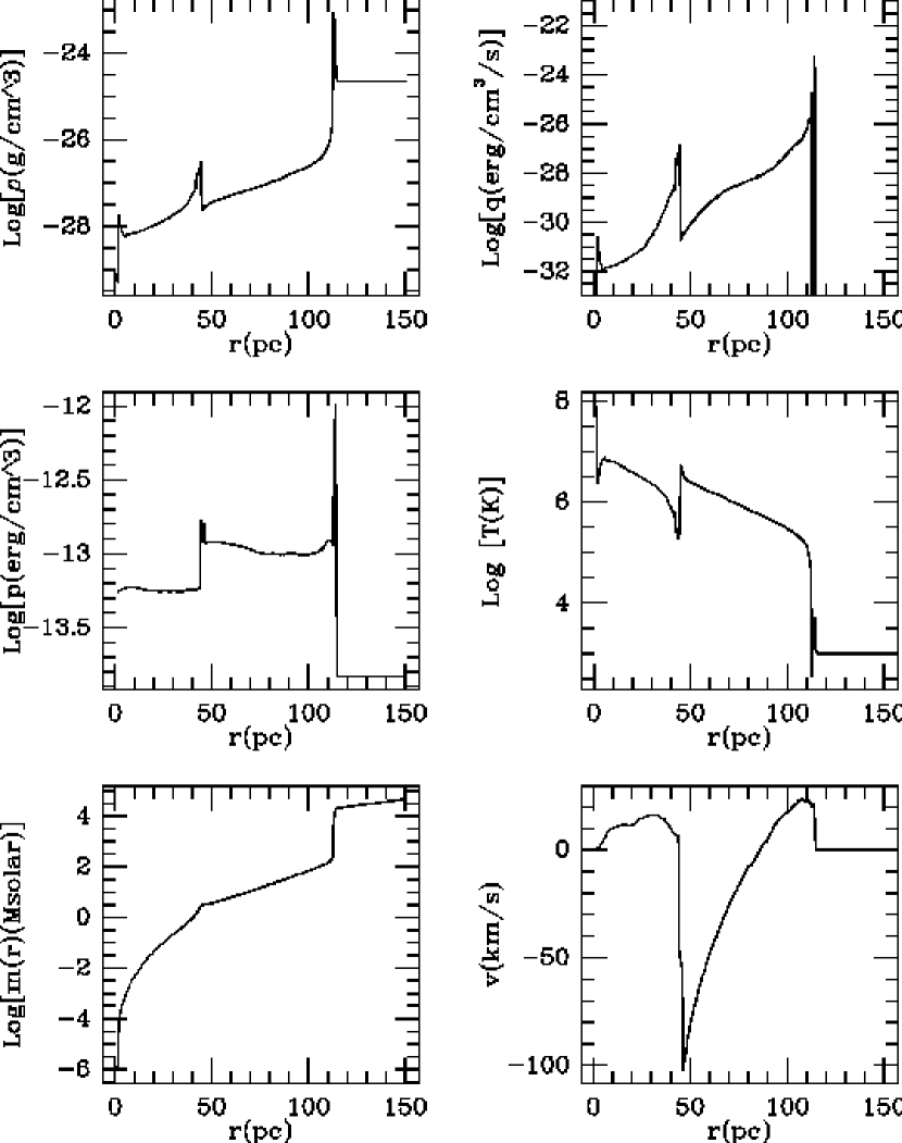
Figure 7: Same as Fig. 5 at $t=1.52\times 10^{6}$ yr.

The representative structural information is given in Figures 4 though 7. Quantities such as density $\rho$, pressure $p$, cumulative mass $m(r)$, luminosity per unit volume or cooling rate $q$, temperature $T$, and fluid velocity $V$, are plotted as a function of radius $r$, at times $t=9810$, $1.27\times 10^{5}$, $2.54\times 10^{5}$, and $1.52\times 10^{6}$ yr. These times were chosen to represent the various phases in the evolution of the SNR. In addition, the Sedov-Taylor solution is plotted with the numerical results of density, pressure, and post-shock fluid velocity for $t=9810$ yr, in order to illustrate the agreement and the disagreement between our numerical results and the Sedov-Taylor solution.

Although some of these phases have previously been studied, we will briefly review the characteristics and governing physical processes in each phase.

3.1.1 Sedov-Taylor Stage

An early phase, where cooling has not been efficient, is represented in Figure 4 (the structure at $t=9810$ yr) and Figure 5 (at $t=1.27\times 10^{5}$ yr). The structure is similar to that of the Sedov-Taylor solution (Sedov 1959, Taylor 1950), which is applicable to the adiabatic expansion of a spherical wave (i.e. explosion starting at an infinitesimally small radius). However, a slight indication of the effect of cooling is already seen at the shock front by $t=1.27\times 10^{5}$ yr; the velocity, density, and pressure are smaller than predicted by the Sedov-Taylor solution. To demonstrate that this deviation is due to cooling, the velocity, the density, and the pressure profiles at an earlier time, when practically no cooling has yet occurred, are compared to the Sedov-Taylor solution in Figure 4. It shows the numerical results (solid lines) and the Sedov-Taylor solution (taken at $t=9808+170$, the approximate age of the SNR at the initial condition, dashed lines). The peak values and the location of the peak values agree well, even though the detailed structure deviates because the numerical solution is influenced by the initial condition of the explosion (with a finite radius), as expected for a realistic calculation. This can be seen easily in the velocity profile, which shows the reverse shock propagating inward. The reverse shock travels to the contact discontinuity, where it is partially transmitted and reflected, and to the center, where it is reflected. The resulting waves eventually catch up and interact with the shock front, influencing the shock structure and the cooling history. Dynamic relaxation can be achieved if much of the initial explosion energy is provided in the form of the thermal energy in a very small volume (thus increasing the sound velocity and shortening the relaxation time), as seen in the results of Chevalier (1974). However, previous studies have shown that the bulk of the explosion energy is put into the motion of the matter, rather than into the thermal energy (see CMB and the references thereof). Therefore, for realistic initial conditions, such as those considered in our study, we do not expect a complete agreement between the numerical results and the Sedov-Taylor solution.

As mentioned earlier, the Sedov-Taylor solution for adiabatic expansion describe the global behavior of quantities like those shown in Fig. 3 quite well. The slope of $\log(R)$ as a function of $\log(t)$ from the numerical calculation is indeed about 2/5 (0.400 with residual sum $=3.45\times 10^{-4}$ for the fit with data between $\log(t[{\rm yr}])=3.7$ and $4.9$ ), as predicted from the analytical solution. The post-shock fluid velocity is related to the shock velocity $V_{s}$ by

$${V_{ps}\over V_{s}}={{\gamma-1}\over{\gamma+1}}+{2\over{(\gamma+1})M^{2}},$$

where $\gamma$ is the effective adiabatic exponent of the gas, and $M$ is the Mach number of the shock, $M^{2}=V_{s}^{2}/c_{s}^{2}$. For a strong shock, the second term is negligible. If there is negligible cooling, the value of $\gamma$ is the same as the ratio of specific heats at constant pressure and at constant volume, $C_{p}/C_{V}$, assumed to be 5/3. This is true during the adiabatic phase, and the ratio $V_{ps}/V_{s}$ stays approximately constant; therefore, the slope of $\log V_{ps}$ is equal to $\log V_{s}$. The slope of $\log V_{ps}$ as a function of $\log t$ in Fig. 3 is about 3/5, consistent with the prediction for $\log V_{s}$ by the analytical solution.

The energies stay approximately constant over this phase, with only slight adjustment in kinetic and thermal energies once they reach the equilibrium value. The distinction between the shell and the bubble is not rigorous during this phase, as the thin shell has not yet formed. Therefore, the values associated with the shell or the bubble should be taken with caution. It is clear from the plots that the dynamical behavior of the SNR is not influenced until the cooling is near the maximum.

3.1.2 Radiative Phase

Toward the end of the Sedov-Taylor phase, the effect of cooling in the density-enhanced shock front region gradually becomes significant and begins to influence the dynamical evolution. The pressure just behind the shock front decreases due to the temperature drop. The system reacts by adjusting the velocity profile. The decrease of the velocity at the shock front compared to the peak velocity value, as seen in the structure at the onset of the radiative phase ($t=2.54\times 10^{5}$ yr, Figure 6), is due to this effect. The temperature drop due to cooling is also clearly seen in the same plot. Due to the pressure drop behind the shock front caused by cooling, the velocity at the shock front decreases. The deceleration is not as large away from the shock front, and therefore the velocity near the shock front creates a tier, where a reverse shock forms (see Fig. 6). The reverse shock, which appears as a cusp in the velocity profile just behind the shock front, travels inwards relative to the shock front to the contact discontinuity (see Fig. 7), reflecting and transmitting at the discontinuity. The transmitted wave travels to the center, where it is reflected. The wave reflected at the contact discontinuity travels back toward the shock front. These waves eventually interact with others to create complex wave patterns over the entire SNR in its late evolution.

As the cooling becomes very efficient and the thin shell forms at the shock front, the remnant moves into the radiative phase. The thermal energy, converted from kinetic energy is radiated away immediately. The density enhancement at the shock front becomes significantly more than the adiabatic (strong shock) value of $(\gamma+1)/(\gamma-1)$. This, in turn, enhances the cooling, which is proportional to the square of the local density. This brings the catastrophic cooling. Much SNR energy is lost in this phase.

It should be emphasized that the fraction of the energy input from a SN to the ISM, which is retained by the ISM, in a solar-like environment, is significantly less than the explosion energy of the SN. It is important to realize that most of such violent energy input escapes in radiation, and therefore does not provide as much energy input to the ISM as it is often assumed. Any study which must include such energy input to the ISM in order to model an evolving stellar system must take into account the radiation loss from the shells of SNRs. We will consider this point in more detail in §5.

3.1.3 Late Phases: Post-Cooling and Momentum-Conserving Snowplow

In the very late stage of the SNR remnant evolution, the shell (where most of the cooling takes place) becomes cold and less dense (due to the weakness of the shock and the cooling), and consequently the total cooling in the SNR becomes less efficient. This phase was not studied by CMB since for their analytical study they assumed a simple power-law cooling function which increases as the temperature decreases (and thus the gas is cooled efficiently to zero temperature, in effect). Also, they only followed the remnant evolution to $1.75\times 10^{6}$ yr. Although the effects of shell cooling have become small by this time, the resulting change in the behavior of SNR characteristics is not obvious until about $4\times 10^{6}$ yr, at which time the accreted thermal energy from the ambient matter becomes larger than the remnant cooling. Only then, the resulting increase in the total thermal energy is clearly seen (See Fig. 3).

In the post-cooling phase, the cooling still continues in the bubble; however, it does not become very efficient due to the low density of the gas outside the shell. The total energy is again (approximately) conserved, as it was in the adiabatic phase. The shell becomes thicker as the rate of cooling in the shell decreases. Eventually, the cooling rate becomes orders of magnitude less than the peak value, and therefore it can be deemed negligible. A representative structure at the transition into this phase ($t=1.52\times 10^{6}$ yr) is shown in Figure 7. This is very close to the time at which the final results were taken for the fits presented in the later section. The structure is characterized by a thick shell with a size of a few parsecs and a complex velocity profile due to wave interactions. The bubble is still hot (T $\approx$ $10^{6}$ K) and very rarefied ($\rho\approx 10^{-28}$ to $10^{-27}{\rm g}/{\rm cm}^{3}$).

The pressure inside the SNR still exceeds the unshocked pressure, although the difference decreases with time. The time at which the interior pressure is no longer significantly larger than the unshocked ambient pressure depends on the temperature, as well as on the density of its environment. At this time, the SNR moves into the momentum-conserving snowplow phase.

In the momentum-conserving snowplow phase, unlike the pressure-driven snowplow (or radiative) phase discussed earlier, there is no longer a “push” from the interior pressure, since the interior and exterior pressures are approximately equilibrated. The momentum is conserved as the SNR continues to evolve. The increases in the total energy and thermal energy at very late times, seen in Fig. 3, are due to the accumulation of the matter and the associated thermal energy in the ambient medium, which is no longer cooled by radiation as it becomes part of the SNR. An analytic solution for this phase is easily obtainable from the equations of motion, energy conservation, momentum conservation, and the equation of state. Our results are not influenced by the existence of this phase because the final results (i.e., when most of the cooling is finished) are taken well before the SNR enters this phase, for a typical ISM pressure.

In some cases, a SNR may become indistinguishable with the ISM (i.e., merge with the ISM) before it reaches the momentum-conserving snowplow phase. In any case, all SNR will merge with the ISM eventually. The most common criterion used to determine when the transition occurs is the equality of the shock velocity with the sound velocity of the ISM. The transition time is thus dependent on the temperature of the ambient medium, as well as on the density.

Our careful examination of the SNR characteristics over the lifetime, combined with the knowledge of treatments of energy input in stellar system formation and evolution, enabled us to determine the best time to take the final characteristics of SNRs. In essence, we have chosen the earliest time at which the enhanced shell cooling due to radiation has ceased in effect: sufficiently early so that late time effects such as the accumulation of ambient thermal energy are small, and sufficiently late so that the luminosity has dropped to a small value. We also used the fact that many SNR characteristics scale well with $t_{0}$, the time at which the maximum luminosity is attained. We have determined from the calculations that all models have luminosities that are less than 0.5% of the corresponding maximum luminosities by the age of $13\times t_{0}$. Therefore, we have chosen to define the final age, $t_{f}$, to be $13\times t_{0}$. At $t_{f}$, the amount of thermal energy which has accumulated from the surroundings (which behaves like the accumulation of the mass) is well below 5% of the thermal energy, and below 1% of the total energy. The final time $t_{f}$, as defined, occurs earlier than both the onset of the momentum-conserving snowplow phase and the merging of the SNR with the ISM, for most interstellar conditions.

3.2 The Effect of Ambient Density

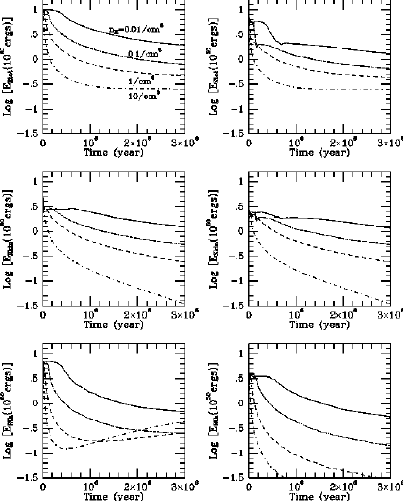
Figure 8: Total energy, kinetic energy, and thermal energy of the SNR ($E_{Rtot}$, $E_{Rkin}$, and $E_{Rth}$, respectively) and total energy, and kinetic energy of the shell ($E_{Stot}$ and $E_{Skin}$, respectively), and thermal energy in the hot bubble $E_{Bth}$ vs. time, for various cases of ambient density ($n_{H}=0.01$ (solid line), $0.1$ (dotted line), $1.0$ (dashed line), and $10.0$ (dash-dotted line) ${\rm cm}^{-3}$). The metallicity is fixed at $Z_{\hbox{$\odot$}}$.

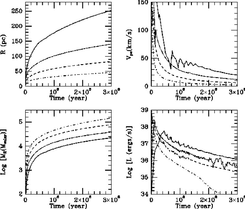
Figure 9: The radius $R$ and the mass of the SNR $M_{R}$, the post-shock fluid velocity $V_{ps}$, and the luminosity of the SNR $L$, as a function of time, for the cases of Fig. 8.

Figures 8 and 9 show various global quantities as functions of time for $Z=0.02$ and several ISM densities. The total energy, the kinetic energy, and the thermal energy of the SNR ($E_{Rtot}$, $E_{Rkin}$, and $E_{Rth}$, respectively), the total energy and the kinetic energy of the shell ($E_{Stot}$ and $E_{Skin}$, respectively), and the thermal energy in the hot bubble $E_{Bth}$ are plotted against time in Fig. 8. The radius $R$ and the mass of the SNR, $M_{R}$, the post-shock fluid velocity, $V_{ps}$, and the luminosity of the SNR, $L$, as a function of time are plotted in Fig. 9. The increase in the total energy at very late times for the high-density case is due to the accumulation of matter and thermal energy from the ambient ISM. This will be discussed in more detail later in this section. For all cases, it is clear that the energy input from a supernova is significantly less than the initial $10^{51}$ ergs, a value which has been assumed in various models of galactic and globular cluster formation and evolution. In addition, the strong dependence of the SNR evolution on the ambient density should be noted. This is due to the fact that the cooling rate is proportional to the square of the local density behind the shock (which is influenced by the pre-shock density values).

In our SNR models, the time scales of cooling vary from about $10^{4}$ yr to a few $10^{5}$ yr. These time-scales are smaller than the size of time steps taken in galactic models, due to the fact that the total evolution time for such models tend to be of the order of 10 Gyr. The numerical restrictions typically limit the total number of time steps to 10,000 to 100,000 time steps, depending on how much computation is involved in each time step. As a result, the time steps in such models are limited to about $10^{5}$ yr at most, much larger than the representative cooling time or dynamical time of SNR evolution. Therefore, it is clear that galactic models cannot resolve the shocks either in time or in space.

The effects of interactions at the shock front with waves created in reflection of the initial reverse shock, discussed in §3.1.1, are best visible in the lowest density case ($\rho_{0}=0.0133{\rm m_{H}}/{\rm cm}^{3}$, solid line in Fig. 8). The evolution time scale is a steep power of $\rho_{0}$, and therefore more wave interactions and details of the early phase can be seen in the lowest density case. A steep decrease in the post-shock fluid velocity indicates the deceleration of the shock front due to the pressure gradient, as a result of strong cooling. The density is enhanced further, resulting in a higher cooling rate. Eventually, the wave created by reflection of initial reverse shock approaches the shock front. As it reaches the shock front, the interaction increases the shock velocity, thereby decreasing the density in the front. This then results in a sudden decrease of the cooling rate. The amplitudes and the velocities of such waves dissipate with time, as they encounter the shell of the contact discontinuity and that of the shock front. Some fraction transmits through the contact discontinuity, travels to the center, and then reflects back, again encountering the contact discontinuity. After a few $t_{0}$, major wave interactions with the shock front are no longer observed.

The highest density case (dash-dotted line in Fig. 8 and 9) is helpful in illustrating the post-cooling phase. When the luminosity L becomes two orders of magnitude less than that of the peak value, it is clear that the thermal energy of the SNR stops decreasing. It reaches to a minimum, stays constant, then starts increasing. This increase is due to the fact that the cooling rate falls below the rate of thermal energy accumulation from the surroundings, in addition to the energy converted from kinetic energy in the shock. The cooling continues mainly in the hot bubble, but at a much lower rate. Cooling in an unshocked medium can be and is currently included in models of stellar systems, as they can easily be resolved both in time and in space. Therefore, the effects of continuing cooling in the bubble and the shell are not considered here, but are left for models of stellar systems to include as cooling of the ISM.

The different behavior exhibited by the various density cases are significant enough that it is necessary to formulate the SN energy input to the ISM as a function of density. We will therefore give a description of SNR properties as a function of the ambient density in §4.

3.3 The Effect of Metallicity

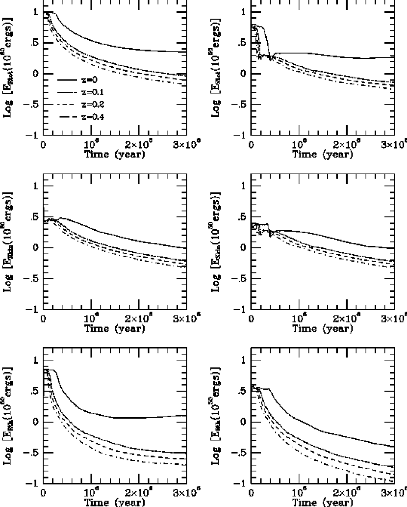
Figure 10: Total energy, kinetic energy, and thermal energy of the SNR ($E_{Rtot}$, $E_{Rkin}$, and $E_{Rth}$, respectively) and total energy, and kinetic energy of the shell ($E_{Stot}$ and $E_{Skin}$, respectively), and thermal energy in the hot bubble $E_{Bth}$ vs. time, for various cases of metallicity ($Z=0.00$ (solid line), $0.01$ (dotted line), $0.02$ (dash line), and $0.04$ (dash-dot line) in the unit of $m_{H}/{\rm cm}^{3}$). The ambient density is fixed at $\rho_{0}=0.133m_{H}/{\rm cm}^{3}$.

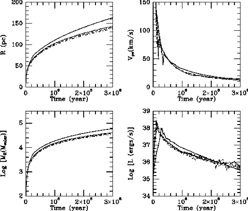
Figure 11: The radius $R$ and the mass of the SNR $M_{R}$, the post-shock fluid velocity $V_{ps}$, and the luminosity of the SNR $L$, as a function of time, for the cases in Fig. 10.

Figures 10 and 11 show the evolution of various global quantities for $\rho_{0}=0.133\,{\rm m_{H}}/{\rm cm}^{3}$ and $Z=0.00$, $0.01$, $0.02$, and $0.04$. The total energy, the kinetic energy, and the thermal energy of the SNR ($E_{Rtot}$, $E_{Rkin}$, and $E_{Rth}$, respectively), total energy and the kinetic energy of the shell ($E_{Stot}$ and $E_{Skin}$, respectively), and the thermal energy in the hot bubble $E_{Bth}$ are plotted against time in Fig. 10. The radius $R$ and the mass of the SNR, $M_{R}$, the post-shock fluid velocity, $V_{ps}$, and the luminosity of the SNR, $L$, as a function of time are plotted in Fig. 11. The low-metallicity case indeed exhibits a slower rate of cooling and a smaller energy loss. Nevertheless, the loss is already significant after 1 Myr, a short time scale compared to the galactic evolution time scale. The neglect of the cooling in the shell is thus inappropriate, even for the case of a zero metallicity environment. The differences in energy evolution between the models stem from the very efficient metal cooling, which leads to considerably larger values of the cooling function at temperatures between $10^{5}$ K and $10^{7}$ K. This illustrates the need to explicitly include the dependence of the supernova energy input on the environmental metallicity. The actual form of this dependence is given in the next section.

The difference is most significant between a case with a moderate amount of metals and the case with very low metallicity ($\log{Z/Z_{\hbox{$\odot$}}}\leq-2$). The time scale of evolution clearly depends on the metallicity. There is a difference of a factor of about three in the time scale between the low-metallicity case and the solar-metallicity case. In addition, more energy is retained if the metallicity is low. These are the consequences of metallicity dependent cooling (see Fig. 1). The highly efficient cooling by metals results in larger values of the cooling function for the higher metallicity cases. On the other hand, the cooling in a low metallicity gas is inefficient, due to the absence of metal cooling.

Note that we have assumed that the cooling functions are calculated with the metallicity of the ISM, not of the ejecta-ISM mixture. The validity of this assumption is strongly suggested by the results of a 2-D calculation (Gaudlitz 1996). Although a significant amount of mixing occurs, the shell of the SNR itself is rather stable during the radiative phase. The mixing is confined to the bubble, where cooling is not efficient due to the low density. The shell consists of freshly accumulated material from the surroundings, and therefore the cooling function need not to be modified. This assumption is examined in detail in §5.1.

4 POWER-LAW FITS FOR THE GLOBAL QUANTITIES

For a simple incorporation of these results to global modeling of stellar/ISM system formation and evolution, we need a set of descriptions for the global quantities, such as the energies and masses of the SNR and the shell. We will now show that the basic dependences of these quantities on metallicity and density are well described by power-law fits. With the use of such power-laws, it is possible to include the effects of the environment in supernova energy input in galaxy or globular cluster formation models. For this purpose, we have widened the range of the densities and the metallicities we explore. We have selected densities ranging from $1.33\times 10^{-3}{\rm m_{H}}/{\rm cm}^{3}$ to $1.33\times 10^{3}{\rm m_{H}}/{\rm cm}^{3}$, and $\log{Z/Z_{\hbox{$\odot$}}}$ ranging from $-3$ to $0.5$. (The values of global quantities for $\log{Z/Z_{\hbox{$\odot$}}}=-3$ is not included in the fit, and thus not plotted in the figures.)

Table 1: Model Results at $t_{0}$ (Dynamical and General Properties)

$\log[\displaystyle{Z\over Z_{\hbox{$\odot$}}}]$	$\rho/m_{H}$	$t_{0}$	$\log(R)$	$\log(M_{R})$	$\log(M_{S})$	$\log(L_{max})$
	$(cm^{-3})$	$(yr)$	$(pc)$	$(g)$	$(g)$	$(erg/sec)$
$-3.0$	$1.33E-01$	$2.88E+05$	$75.4$	$37.090$	$36.943$	$38.20$
$-2.0$	$1.33E-01$	$2.82E+05$	$74.4$	$37.072$	$36.930$	$38.21$
$-1.5$	$1.33E-01$	$2.69E+05$	$73.3$	$37.052$	$36.909$	$38.24$
$-1.0$	$1.33E-01$	$2.34E+05$	$69.1$	$36.976$	$36.824$	$38.16$
$-0.5$	$1.33E-01$	$1.64E+05$	$59.9$	$36.814$	$36.675$	$38.23$
$0.5$	$1.33E-01$	$8.87E+04$	$47.9$	$36.511$	$36.339$	$38.71$
$0.0$	$1.33E-03$	$1.43E+06$	$368.3$	$37.166$	$37.003$	$36.96$
$0.0$	$1.33E-02$	$4.22E+05$	$142.7$	$36.929$	$36.751$	$37.74$
$0.0$	$1.33E-01$	$1.22E+05$	$55.8$	$36.715$	$36.542$	$38.48$
$0.0$	$1.33E+00$	$3.44E+04$	$21.4$	$36.473$	$36.282$	$39.22$
$0.0$	$1.33E+01$	$9.73E+03$	$8.2$	$36.223$	$36.033$	$39.79$
$0.0$	$1.33E+02$	$3.06E+03$	$3.3$	$36.011$	$35.838$	$40.42$
$0.0$	$1.33E+03$	$9.57E+02$	$1.3$	$35.798$	$35.630$	$40.96$

Table 1—Continued: Model Results at $t_{0}$ (Energetics)

$\log[\displaystyle{Z\over Z_{\hbox{$\odot$}}}]$	$\rho/m_{H}$	$\log(E_{Rtot})$	$\log(E_{Stot})$	$\log(E_{Rkin})$	$\log(E_{Skin})$	$\log(E_{Rth})$	$\log(E_{Bth})$
	$(cm^{-3})$	$(erg)$	$(erg)$	$(erg)$	$(erg)$	$(erg)$	$(erg)$
$-3.0$	$1.33E-01$	$50.907$	$50.605$	$50.463$	$50.384$	$50.713$	$50.552$
$-2.0$	$1.33E-01$	$50.894$	$50.588$	$50.456$	$50.376$	$50.697$	$50.541$
$-1.5$	$1.33E-01$	$50.888$	$50.573$	$50.462$	$50.378$	$50.683$	$50.541$
$-1.0$	$1.33E-01$	$50.866$	$50.529$	$50.454$	$50.357$	$50.654$	$50.532$
$-0.5$	$1.33E-01$	$50.896$	$50.603$	$50.434$	$50.345$	$50.713$	$50.528$
$0.5$	$1.33E-01$	$50.857$	$50.491$	$50.416$	$50.293$	$50.662$	$50.539$
$0.0$	$1.33E-03$	$50.923$	$50.610$	$50.421$	$50.295$	$50.759$	$50.561$
$0.0$	$1.33E-02$	$50.891$	$50.535$	$50.422$	$50.294$	$50.711$	$50.565$
$0.0$	$1.33E-01$	$50.870$	$50.562$	$50.418$	$50.332$	$50.681$	$50.518$
$0.0$	$1.33E+00$	$50.852$	$50.523$	$50.426$	$50.336$	$50.647$	$50.515$
$0.0$	$1.33E+01$	$50.884$	$50.588$	$50.438$	$50.368$	$50.691$	$50.528$
$0.0$	$1.33E+02$	$50.904$	$50.633$	$50.436$	$50.371$	$50.723$	$50.523$
$0.0$	$1.33E+03$	$50.888$	$50.641$	$50.428$	$50.363$	$50.703$	$50.474$

Table 2: Model Results at $t_{f}$ (Dynamical and General Properties)

$\log[\displaystyle{Z\over Z_{\hbox{$\odot$}}}]$	$\rho/m_{H}$	$t_{f}$	$\log(R)$	$\log(M_{R})$	$\log(M_{S})$	$\log(L_{f})$	$\log(\displaystyle{L_{f}\over L_{max}})$
	$(cm^{-3})$	$(yr)$	$(pc)$	$(g)$	$(g)$	$(erg/sec)$
$-3.0$	$1.33E-01$	$3.74E+06$	$175.6$	$38.181$	$38.166$	$35.35$	$-2.85$
$-2.0$	$1.33E-01$	$3.67E+06$	$171.2$	$38.152$	$38.137$	$35.85$	$-2.36$
$-1.5$	$1.33E-01$	$3.50E+06$	$163.5$	$38.089$	$38.075$	$35.91$	$-2.33$
$-1.0$	$1.33E-01$	$3.04E+06$	$150.3$	$37.992$	$37.981$	$35.95$	$-2.21$
$-0.5$	$1.33E-01$	$2.13E+06$	$129.5$	$37.812$	$37.800$	$36.14$	$-2.09$
$0.5$	$1.33E-01$	$1.15E+06$	$99.5$	$37.483$	$37.470$	$36.31$	$-2.40$
$0.0$	$1.33E-03$	$1.86E+07$	$803.4$	$38.183$	$38.158$	$35.16$	$-1.80$
$0.0$	$1.33E-02$	$5.49E+06$	$301.6$	$37.916$	$37.900$	$35.70$	$-2.04$
$0.0$	$1.33E-01$	$1.59E+06$	$114.3$	$37.647$	$37.630$	$36.18$	$-2.30$
$0.0$	$1.33E+00$	$4.47E+05$	$43.0$	$37.386$	$37.371$	$36.63$	$-2.59$
$0.0$	$1.33E+01$	$1.26E+05$	$16.4$	$37.147$	$37.131$	$37.19$	$-2.60$
$0.0$	$1.33E+02$	$3.98E+04$	$6.6$	$36.923$	$36.907$	$37.91$	$-2.51$
$0.0$	$1.33E+03$	$1.24E+04$	$2.5$	$36.793$	$36.783$	$38.26$	$-2.70$

Table 2—Continued: Model Results at $t_{f}$ (Energetics)

$\log[\displaystyle{Z\over Z_{\hbox{$\odot$}}}]$	$\rho/m_{H}$	$\log(E_{Rtot})$	$\log(E_{Stot})$	$\log(E_{Rkin})$	$\log(E_{Skin})$	$\log(E_{Rth})$	$\log(E_{Bth})$
	$(cm^{-3})$	$(erg)$	$(erg)$	$(erg)$	$(erg)$	$(erg)$	$(erg)$
$-3.0$	$1.33E-01$	$50.332$	$50.262$	$49.921$	$49.917$	$50.118$	$49.488$
$-2.0$	$1.33E-01$	$50.266$	$50.187$	$49.924$	$49.919$	$50.002$	$49.472$
$-1.5$	$1.33E-01$	$50.159$	$50.059$	$49.904$	$49.896$	$49.808$	$49.457$
$-1.0$	$1.33E-01$	$50.119$	$50.017$	$49.924$	$49.920$	$49.678$	$49.427$
$-0.5$	$1.33E-01$	$50.117$	$50.006$	$49.952$	$49.947$	$49.616$	$49.454$
$0.5$	$1.33E-01$	$50.035$	$49.950$	$49.924$	$49.921$	$49.389$	$49.273$
$0.0$	$1.33E-03$	$50.242$	$50.105$	$49.987$	$49.968$	$49.890$	$49.635$
$0.0$	$1.33E-02$	$50.135$	$50.024$	$49.958$	$49.954$	$49.658$	$49.472$
$0.0$	$1.33E-01$	$50.040$	$49.932$	$49.903$	$49.888$	$49.473$	$49.330$
$0.0$	$1.33E+00$	$49.967$	$49.905$	$49.881$	$49.877$	$49.222$	$49.067$
$0.0$	$1.33E+01$	$49.972$	$49.939$	$49.924$	$49.923$	$48.988$	$48.807$
$0.0$	$1.33E+02$	$49.915$	$49.894$	$49.883$	$49.882$	$48.755$	$48.550$
$0.0$	$1.33E+03$	$50.048$	$50.041$	$50.035$	$50.034$	$48.506$	$48.177$

In order to obtain a realistic measure of the cooling in the shell created by shocks, the final model was taken at $t_{f}=13\times t_{0}$, where $t_{0}$ is the age of SNR at the maximum luminosity (or maximum cooling rate). This value was chosen such that the models have a luminosity of approximately 0.5% of the maximum value by this time. The cooling continues slowly; such effect must be taken into account separately as a cooling of the (unshocked) ISM in any application of our results.

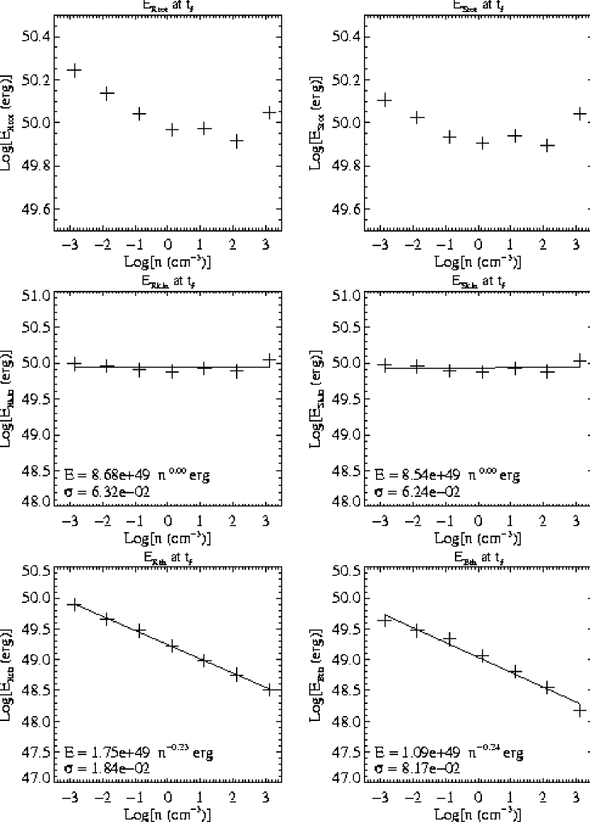
Figure 12: The global quantities relevant for prescribing the effects of SN explosions on the surrounding ISM as a function of the ambient density, and the least-square fits are shown where appropriate. The quantities are total energy, kinetic energy, and thermal energy of the SNR ($E_{Rtot}$, $E_{Rkin}$, and $E_{Rth}$, respectively) and total energy, and kinetic energy of the shell ($E_{Stot}$ and $E_{Skin}$, respectively), and thermal energy in the hot bubble $E_{Bth}$. All quantities are taken at $t_{f}$, defined by $13\times t_{0}$, where $t_{0}$ is the time the maximum luminosity is attained. The metallicity is fixed at $Z_{\hbox{$\odot$}}$. $\sigma$ is the standard deviation.

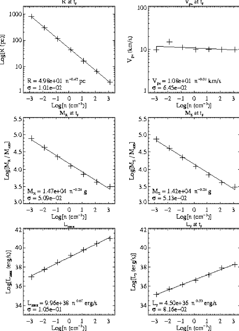
Figure 13: Similar to Fig. 12. Quantities plotted and fitted are the radius $R$, the total mass $M_{R}$, the maximum luminosity attained $L_{max}$, the post-shock fluid velocity $V_{ps}$, the shell mass $M_{S}$, and the luminosity $L_{f}$. All quantities except for $L_{max}$ are taken at $t_{f}$ (See Fig. 12). The metallicity is fixed at $Z_{\hbox{$\odot$}}$.

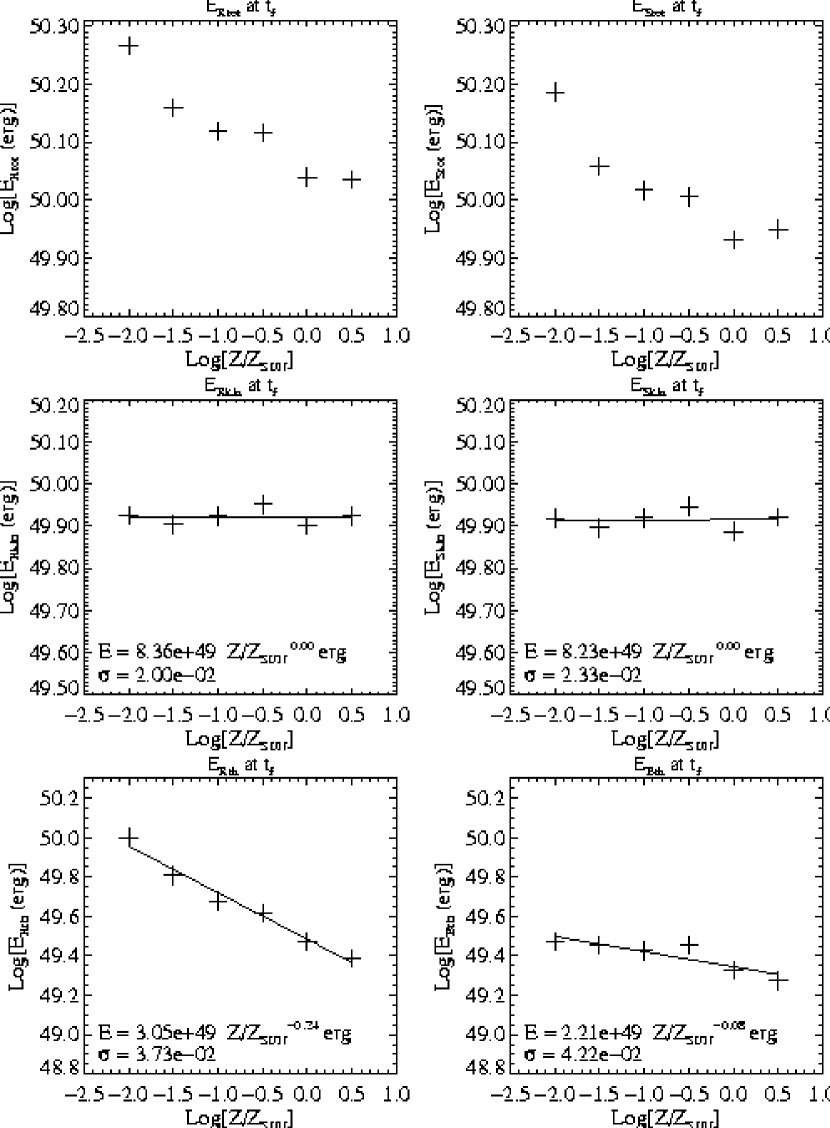
Figure 14: Same as in Fig. 12, but they are plotted as a function of the ambient metallicity $Z/Z_{\hbox{$\odot$}}$. The ambient density is fixed at $\rho_{0}=0.133m_{H}/{\rm cm}^{3}$.

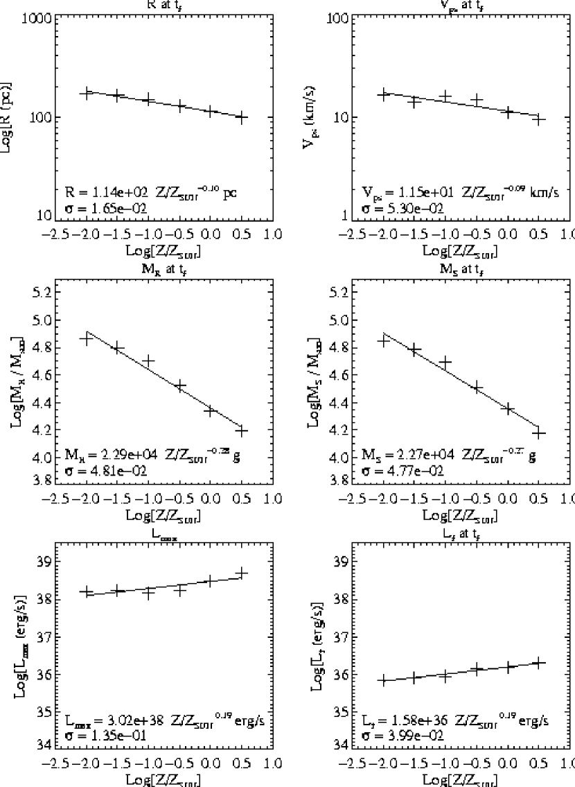
Figure 15: Same as in Fig. 13, but they are plotted as a function of the ambient metallicity $Z/Z_{\hbox{$\odot$}}$. The ambient density is fixed at $\rho_{0}=0.133m_{H}/{\rm cm}^{3}$.

Based upon the results from our numerical calculations for SNRs in different density and metallicity environments, we can now identify the dependences of critical quantities on those parameters. The results are presented in two ways. First, Table 1 and 2 contain all of the values of global properties at $t_{0}$ and $t_{f}$, respectively. Second, power-law fits were constructed for the results. Figures 12 through 15 illustrate the fits obtained.

The energies of the early supernova remnant evolution are almost constant across the range of environmental density and metallicity we have explored, as seen in Table 1. This indicates that the SN evolves almost adiabatically until about $t_{0}$. The metallicity and density dependent cooling has not affected the SNRs to this stage. On the other hand, the dependences of cooling on metallicity and density are clearly seen in Table 2, taken at $t_{f}$. For this table, the number of significant digits is determined so that the difference between SNR quantities (e.g., $M_{R}$) and shell (or bubble) quantities (e.g., $M_{S}$) is a well- determined number. Those differences can be very small, and keeping fewer digits would have yielded zero, due to rounding. The number of the digits does not reflect the accuracy, but they are chosen for practical purposes.

The fit with metallicity was split into two parts because of the nonlinear dependence of cooling on metallicity. Near $\log(Z/Z_{\hbox{$\odot$}})=-2$ and below, the cooling is dominated by hydrogen and helium, and therefore the strong dependence of the cooling efficiency on the metallicity disappears (see Fig. 1). For $\log(Z/Z_{\hbox{$\odot$}})>-2$, the strong metallicity dependence of the cooling efficiency manifests itself in almost all global quantities plotted in Figures 14 and 15 .

The fits for all quantities of interest at $t_{f}$ are presented for $\log[Z/Z_{\hbox{$\odot$}}]>-2$ in the first column below. For $\log[Z/Z_{\hbox{$\odot$}}]\leq-2$, the metallicity dependence disappears; the corresponding fits are given in the second column.

$${\log[Z/Z_{\hbox{$\odot$}}]>-2}$$

$$E_{Rtot}=E_{Rkin}+E_{Rth}$$

$$E_{Rkin}=8.52\times 10^{49}E_{51}{\rm ergs}$$

$$E_{Rth}=1.83\times 10^{49}E_{51}n_{0}^{-0.23}(Z/Z_{\hbox{$\odot$}})^{-0.24}{\rm ergs}$$

$$E_{Stot}=E_{Skin}+(E_{Rth}-E_{Bth})$$

$$E_{Skin}=8.39\times 10^{49}E_{51}{\rm ergs}$$

$$E_{Bth}=1.23\times 10^{49}E_{51}n_{0}^{-0.24}(Z/Z_{\hbox{$\odot$}})^{-0.08}{\rm ergs}$$

$$R=49.3E_{51}^{2/7}n_{0}^{-0.42}(Z/Z_{\hbox{$\odot$}})^{-0.1}pc$$

$$M_{R}=1.44\times 10^{4}E_{51}^{6/7}n_{0}^{-0.24}(Z/Z_{\hbox{$\odot$}})^{-0.28}M_{\hbox{$\odot$}}$$

$$M_{S}=1.41\times 10^{4}E_{51}^{6/7}n_{0}^{-0.24}(Z/Z_{\hbox{$\odot$}})^{-0.27}M_{\hbox{$\odot$}}$$

$$V_{s}=11.3E_{51}^{1/14}n_{0}^{-0.01}(Z/Z_{\hbox{$\odot$}})^{-0.09}km/s$$

$$L=4.55\times 10^{36}E_{51}^{11/14}n_{0}^{0.53}(Z/Z_{\hbox{$\odot$}})^{0.19}erg/s$$

$${\log[Z/Z_{\hbox{$\odot$}}]}\leq-2$$

$$E_{Rtot}=E_{Rkin}+E_{Rth}$$

$$E_{Rkin}=8.52\times 10^{49}E_{51}{\rm ergs}$$

$$E_{Rth}=5.53\times 10^{49}E_{51}n_{0}^{-0.23}{\rm ergs}$$

$$E_{Stot}=E_{Skin}+(E_{Rth}-E_{Bth})$$

$$E_{Skin}=8.39\times 10^{49}E_{51}{\rm ergs}$$

$$E_{Bth}=1.78\times 10^{49}E_{51}n_{0}^{-0.24}{\rm ergs}$$

$$R=78.1E_{51}^{2/7}n_{0}^{-0.42}pc$$

$$M_{R}=5.23\times 10^{4}E_{51}^{6/7}n_{0}^{-0.24}M_{\hbox{$\odot$}}$$

$$M_{S}=4.89\times 10^{4}E_{51}^{6/7}n_{0}^{-0.24}M_{\hbox{$\odot$}}$$

$$V_{s}=17.1E_{51}^{1/14}n_{0}^{-0.01}km/s$$

$$L=1.90\times 10^{36}E_{51}^{11/14}n_{0}^{0.53}{\rm ergs}/{\rm s}$$

In these expressions, $E_{51}$ is the initial explosion energy in $10^{51}$ ergs, and $n_{0}$ is defined by $\rho_{0}/{m_{H}}$. Other quantities are as defined earlier. The initial energy dependence was determined from test runs, and was found to be consistent with the existing studies of CMB and others. The validity of such solutions comes from the fact that the dynamical state of the final stage is still dominated by the pressure-driven snowplow phase of evolution, as the final time marks approximately the end of the pressure-driven snowplow phase. For this reason, we have adopted the exponents from the previous studies, which are very close to our numerical results. A simple analysis shows that the exponent of $E_{51}$ is a slowly varying function of the metallicity (Cioffi & Shull 1991), but we will ignore this effect here since it is small compared to other uncertainties involved.

There is an upward systematic error in the energy, which increases as the density decreases. The source is the thermal energy contributed by the ambient medium. For the worst case (i.e., the lowest density case), this error is estimated to be about 3% of the final total energy.

It should be cautioned that the results so far are purely empirical. The dependences of these quantities on $n_{0}$ and $Z$ have no analytical bases. Therefore, any extrapolation of the results into regions of parameter space beyond that which we have explored in this paper should be done with caution.

5 DISCUSSION

5.1 Validity and Possible Consequences of Assumptions

We have made every effort throughout this study of supernova remnant evolution to insure that we have employed the best available input physics and that our numerical results are accurate. In this section, we comment briefly on the assumptions we have made and the constraints they might impose on the applicability of our results.

We did not include the effects of magnetic fields, as mentioned in §2.1. This assumption is justified if the Alfvén speed is negligible compared to the shock velocity, or in other words, if the post-shock pressure is much greater than the magnetic pressure. Whether this condition is met or not depends upon the strength of the magnetic fields in the ISM. Currently, we do not know how magnetic fields are created in the Universe, and how the strength evolves during the lifetime of galaxies. Therefore, we have chosen not to include magnetic fields in these calculations. Examples of effects of magnetic fields are slower expansion, a smaller final radius, and less energy loss (due to less compression of the shell); that is, the SNR influenced by the (random) magnetic fields of its surroundings would keep more energy, but stay compact (Slavin & Cox 1992). It should be noted that the magnetic fields would play a role to some extent in the evolution of SNRs in the present-day solar environment, with its estimated field strength of about $5\mu G$, as suggested by the authors.

We have also ignored the effects of turbulence by assuming spherical symmetry of the SNR. However, signatures of instabilities are seen in observed young SNRs (Bartel, et al. 1987, 1991; Wilkinson & de Bruyn 1990). The stability of the thin shell has been questioned and studied by others (Gull 1973; Chevalier, Blondin, & Emmering 1992; Chevalier & Blondin 1995). Here, we merely discuss the consequences of non-sphericity with respect to the global dynamics and energetics of SNRs.

Turbulence is important in two aspects. First, the shell, which is assumed to be stable, may become unstable and change the dynamical properties of the SNR. This may, as a result, change the cooling history of the SNR, and therefore the energetics. Secondly, turbulence facilitates mixing, which brings the metal rich ejecta into the material which was accreted from the surroundings. The cooling rate would change only if the turbulence were to carry a significant amount of metals into the shell.

As it was pointed out in §3.3, a 2-D hydrodynamic code was used by Gaudlitz (1996) to calculate the evolution of SNRs similar to the ones we considered here. Their calculation showed that mixing was confined to the bubble, and that the shell is stable for the time scales of interest in our study. The validity of this result relies on whether the spherically symmetric initial condition assumed in the model is satisfactory. In reality, turbulence would have already been established in the SNR and in its shell by the age the model is initially started. It is difficult to predict how turbulence in the very young SNR influence the subsequent evolution. In addition, the stability of the shell changes as its structure changes dynamically. This may be an issue which needs more attention in the future.

We believe that significant mixing of metals into the shell is quite unlikely except at the very early and late phases, independent of the 2-D results. The radial velocity profiles in various stages of SNR evolution suggest that the ejecta enriched material has substantially less radial velocity than the shell, making it difficult for the enriched material to catch up with it. In the ejecta-dominated phase, we expect mixing to occur easily because there is not a large layer of accreted ambient matter between the ejecta and the shell. We also expect a Rayleigh-Taylor instability due to the density and velocity structure. In the very late phases, the shock velocity can become quite small, and more efficient mixing may take place. However, the density in the extended bubble is much less than that of the thin shell, and therefore, the variation in the cooling rate would not change the dynamics nor the energetics noticeably. In any case, our final shell characteristics are extracted before the models reach this phase, and therefore it would not make a significant difference in the results presented in §4.

We have ignored the effects of thermal conduction. In the figures of the structures (Fig. 4 though 7), the temperature profile shows non-uniform structure inside the remnant. In reality, thermal conduction will smooth the profile, keeping it approximately uniform in the inner region, away from the shell (Chevalier 1975; Solinger, Buff, & Rappaport 1975). This does not change the overall behavior of the remnant significantly, since the dominant dynamical and cooling processes occur in and near the shell of the remnant.

In addition, the contact discontinuity seen at r = 8 pc in Fig. 4 ($t=9810$ yr) and at r = 15 pc in Fig. 5 ($t=1.27\times 10^{5}$ yr) is smeared by the effects of thermal conduction, as is the temperature profile. Although the higher density at the contact discontinuity causes extra cooling, it is more than two orders of magnitude less than the value at the shock front, and therefore, does not affect the global cooling history. Therefore, the global characteristics of the SNR are not significantly affected by the approximation to ignore thermal conduction.

5.2 Implications of the Results

The major implication of our results is that the assumptions made in incorporating the energy input from SN explosions to galaxy/globular cluster formation and evolution models should be reconsidered. First, the value of energy input per SN is often overestimated by a factor of about 10. Secondly, the ratio between the amounts that become kinetic energy and thermal energy is not correctly estimated, since the values are often determined from a phase of the SNR that is too early in its evolution. Finally, the effect of the ambient medium on the SNR evolution, which influences the above quantities, is not taken into account. In addition, other effects of SNe on the ISM, such as the production of clouds in the shell, are not taken into account consistently.

We will now give a few specific examples from existing studies of galactic formation/evolution.

Chemodynamical models (Theis, Burkert & Hensler 1992, Burkert, Hensler & Truran 1992) combine dynamical modeling of galaxies with microphysics of the ISM and effects of star formation and evolution to produce results which predict the dynamical state of a galaxy, as well as the chemical compositions. It is a powerful method in studying the history of the Galaxy, giving considerably more information than the studies of dynamics or chemistry separately. The results typically include the chemical compositions and kinematical information as functions of location. Given observational data for comparisons to restrict the model parameters or assumptions, they provide a significantly more reliable history of formation and evolution of galaxies.

Because of its complex nature, there are several simplifying assumptions one must make in such modeling. To treat SN explosions without resolving the shocks, one must assume how much energy is provided, where (e.g., in the cloud or in the hot medium) and in what form (kinetic or thermal). In those studies, it was assumed that the SN explosion provides $10^{51}$ ergs. Unfortunately, the assumed values of the energy input from each SN were overestimated in some studies because they were taken to be equal to the typical total energy released from a SN. In Theis et al. (1992), it was indicated that a factor of five change in the value of $E_{SN}$, the amount of energy input from a SN to the ISM, significantly changes the kinematics. As an example, the resulting velocity dispersion of low mass stars varied from 9 km/s ($E_{SN}=10^{51}{\rm ergs}$) to 78 km/s ($E_{SN}=5\times 10^{51}{\rm ergs}$). The resolution was on a much coarser scale to accommodate the galactic scale, and therefore SN shocks were not resolved. As a result, the cooling in the shell of a SNR was not taken into account, and too much SN energy was put into the ISM.

Cole et al. (1994) performed a extensive search in the parameter space of galactic models by observational fits. One of the parameters they examined was the fraction of supernova energy input that is in the form of kinetic energy, $f_{v}$ (assuming each supernova gives out $10^{51}\rm{ergs}$ in total energy). They concluded that the supernova feedback has a significant influence in their results if $f_{v}$ is of the order of 0.1. They give a best fit value of 0.2, although the model results for $f_{v}=0.1$ and for $f_{v}=0.2$ differ only slightly. Our results indicate a value of about 0.09, which agrees with their conclusion.

In other studies, the value for the supernova energy input is assumed to be a certain number, or related, usually by a constant factor, to the energy input from stellar winds (e.g., Rosen & Bregman 1996). In reality, those values depend largely on the star formation history. In addition, the resolution in their model was better than those in the models mentioned earlier, but it is still not sufficient to resolve the thin shell created in the radiative shock. Thus, such a treatment needs further refinement.

For studies which concern the formation of galaxies or their evolution over a large range of age and metallicity, the treatment of supernovae should include the dependence on the metallicity. No study so far took this effect into account, as well as the dependence on the ambient density. In order to make models of galaxies robust, the dependences need to be considered.

6 CONCLUSIONS

The significant conclusions to be drawn from the numerical studies presented in this paper are the following:

1. The value of supernova energy input in standard assumptions made for the incorporation of the SN energy input into models for the evolution of galaxies is often overestimated. It commonly assumed that the energy input is comparable to the $\approx$ $10^{51}$ ergs associated with the light curve and kinetic energy output of both Type Ia and Type II supernovae. We took this number as the total initial (kinetic plus thermal) energy in our SNR models, and found that much of the energy is lost in radiation. The results are summarized in Table 2 for the energetics of the remnants in the late stages of their expansion. The total energies range from $\approx 9\times 10^{49}$ to $\approx 3\times 10^{50}$ ergs, with a typical case being $\approx$ 10⁵⁰ erg, approximately 10% of the initial total energy.

2. The amount of supernova energy input is a sensitive function of the characteristics – the density and the metallicity – of the environment. The basic dependences are again evident from the model results presented in Table 2. The general trends in these cases are relatively straightforward to understand. The total energy available in kinetic and thermal energy is greatest in the limits of low density and low metallicity. This is a direct consequence of the lower cooling rates that occur in these limits such that a greater fraction of the initial supernova input energy remains in the remnant.

3. A proper treatment of the problem permitting a realistic measure of the relative amounts of thermal energy and kinetic energy is important. The bulk of the supernova energy input provides the kinetic energy of cloud motion. The kinematical properties of clouds are directly related to the kinematical characteristics of stars formed in these clouds. On the other hand, the fraction of the energy in the bubble keeps the gas hot for the time scale of interest. Therefore, mishandling the relative energy input may cause an overestimation of the thermal energy input and an underestimation of the kinetic energy input, or vise versa, changing the model predictions.

4. A proper treatment of the problem permitting a realistic estimate of the relative amounts of shell (cloud) energy and bubble (hot gas) energy is important. As mentioned above, the proper energy divisions into kinetic and thermal energy is critical. Since many galactic models distinguish a cloudy medium and hot medium, the proper method for distributing the total energy input from supernovae becomes important.

5. Furthermore, it has been demonstrated that supernova explosions create a cloudy medium by enhancing the density and thus the cooling in the shock shell, as well as providing a hot, low-density gas. Therefore, we have provided a simplified description of our results, which allows a more realistic treatment of energy input and the mass redistribution by supernovae.

This research began as an attempt to provide an improved measure of the consequences of supernova energy input for the class of models of galactic evolution which attempt to take heating and cooling effects into account properly. There are indeed a number of important problems for which a careful treatment of supernova input is essential. This includes the formation and early evolution of galaxies, where supernova energy input may cause significant mass loss, as possibly reflected in the approximately solar metallicity of the hot gas observed in X-ray emission from clusters of galaxies (Mushotzky et al. 1996). In addition, the supernova energy input is likely to have implications for the abundance evolution of starburst nucleus galaxies (Coziol 1997). In the context of models of self-enrichment, it may also prove to be relevant to the interpretation of the metallicity distributions of globular clusters. Furthermore, energy input due to supernovae has been suggested to cure some shortcomings in hierarchical scenarios of galaxy formation, e.g. the overcooling problem (White & Rees 1978) or the angular momentum problem of disk galaxies (Navarro & Steinmetz 1997).

A critical implication of our results is the quantity of metals produced per unit energy input by supernovae; if the realistic energy input from a supernova is $\approx~{}10^{50}$ ergs rather than $\approx~{}10^{51}$ ergs, approximately 10 times as much metals may be produced per unit supernova energy input. If supernovae are the major source of energy, this result has direct implications for the interplay of chemical and dynamical evolution of the environment.

- (1)
- (2) Abbott, D. C. 1982, ApJ, 263, 723.
- (3)
- (4) Bartel, N. et al. 1987, ApJ, 323, 505.
- (5)
- (6) Bartel, N., Rupen, M. P., Shapiro, I. I., Preston, R. A., & Ruis, A. 1987, Nature, 350, 212.
- (7)
- (8) Böhringer, H., & Hensler, G. 1989, A&A, 215, 147.
- (9)
- (10) Burkert, A., Truran, J. W., & Hensler, G. 1992, ApJ, 391, 651.
- (11)
- (12) Chevalier, R. A. 1974, ApJ, 188, 501.
- (13)
- (14) Chevalier, R. A., & Gardner, J. 1974, ApJ, 192, 457.
- (15)
- (16) Chevalier, R. A. 1975, ApJ, 198, 355.
- (17)
- (18) Chevalier, R. A. 1984, ApJ, 280, 797.
- (19)
- (20) Chevalier, R. A., Blondin, J. M., & Emmering, R. T. 1992, ApJ, 392, 118.
- (21)
- (22) Chevalier, R. A., & Blondin, J. M. 1995, ApJ, 444, 312.
- (23)
- (24) Cioffi, D. F., McKee, C. F., & Bertschinger, E. 1988, ApJ, 334, 252 (CMB).
- (25)
- (26) Cioffi, D. F., & Shull, J. M. 1991, ApJ, 367, 96.
- (27)
- (28) Cole, S., Aragón-Salamanca, A., Frenk, C. S., Navarro, J. F., & Zepf, S. E. 1994, MNRAS271, 781.
- (29)
- (30) Cowie, L. L., Songaila, A., Kim, T.-S., & Hu, E. M. 1995, AJ, 109, 1522.
- (31)
- (32) Cox, D. P. 1972, ApJ, 178, 159.
- (33)
- (34) Cox, D. P., & Smith, B. W. 1974, ApJ, 189, L105.
- (35)
- (36) Coziol, R. 1996, A&A309, 345.
- (37)
- (38) Dalgarno, A. & McCray, R. A. 1972, ARA&A, 10, 375.
- (39)
- (40) Gaudlitz, M. 1996, Diploma Thesis, Technische Universität München.
- (41)
- (42) Gull, S. F. 1973, MNRAS, 161, 47.
- (43)
- (44) Hamilton, A. J. S., & Sarazin, C. L. 1984, ApJ, 281, 682.
- (45)
- (46) Hellsten, U., & Sommer-Larsen, J. 1995, ApJ, 453, 264.
- (47)
- (48) Ikeuchi, S., Habe, A., & Tanaka, Y. 1984, MNRAS, 207, 909.
- (49)
- (50) Janka, H.-Th., Zwerger, Th., & Mönchmeyer, R. 1993, A&A, 268, 360.
- (51)
- (52) Katz, N. 1992, ApJ, 391, 502.
- (53)
- (54) Kazhdan, Ya., & Murzina, M. 1992, ApJ, 400, 192.
- (55)
- (56) Leitherer, C., Robert, C., & Drissen, L. 1992, ApJ, 401, 596.
- (57)
- (58) Lauroesch, J. T., Truran, J. W., Welty, D. E., & York, D. G. 1995, PASP, 108, 641.
- (59)
- (60) Lu, L., Sargent, W. L. W., Barlow, T. A., Churchill, C. W., & Vogt, S. S. 1996, ApJS, 107, 475.
- (61)
- (62) McKee, C. F., & Ostriker, J. P. 1977, ApJ, 218, 148.
- (63)
- (64) McKee, C. F., & Truelove, J. K. 1995, Physics Reports, 256, 157.
- (65)
- (66) McWilliam, A., Preston, G. W., Sneden, C., & Searle, L. 1995, AJ, 109, 2757.
- (67)
- (68) Mushotzky, R. et al. 1996. ApJ, 466, 686.
- (69)
- (70) Navarro, J. F., & Steinmetz,M. 1997, ApJ, 478, 13.
- (71)
- (72) Navarro, J. F., & White, S. D. M. 1993, MNRAS, 265, 271.
- (73)
- (74) Padoan, P., Jimenez, R., & Jones, B. 1997, MNRAS, 285, 711.
- (75)
- (76) Pettini, M., King, D. L., Smith, L. J., & Hunstead, R. W. 1997, ApJ, 478, 536.
- (77)
- (78) Rauch, M., Haehnelt, M. G., & Steinmetz, M. 1997, ApJ, 481, 601.
- (79)
- (80) Rosen, A., & Bregman, J. N. 1995, ApJ, 440, 634.
- (81)
- (82) Ryan, S. G., Norris, J. E., & Beers, T. C. 1996, ApJ, 471, 254.
- (83)
- (84) Sedov, L. I. 1959, Similarity and Dimensional Methods in Mechanics (New York; Academic Press)
- (85)
- (86) Slavin, J. D., & Cox, D. P. 1992, ApJ, 392, 131.
- (87)
- (88) Slavin, J. D., & Cox, D. P. 1993, ApJ, 417, 187.
- (89)
- (90) Solinger, A., Buff, J., & Rappaport, S. 1975, ApJ, 201, 381.
- (91)
- (92) Spicer, D. S., Clerk, R. W., & Maran, S. P. 1990, ApJ, 356, 549.
- (93)
- (94) Steinmetz, M., & Müller, E. 1995, MNRAS, 276, 549.
- (95)
- (96) Sutherland, R., & Dopita, M. A. 1993, ApJS, 88, 253.
- (97)
- (98) Taylor, G. I. 1950, Proc. R. Soc. London A, 201, 159.
- (99)
- (100) Theis, Ch., Burkert, A., & Hensler, G. 1992, A&A, 265, 465.
- (101)
- (102) Timmes, F. X., Lauroesch, J. T., & Truran, J. W. 1995, ApJ, 451, 468.
- (103)
- (104) Tscharnuter, W. M., & Winkler K.-J. 1979, Comp. Phys. Comm. 18, 171.
- (105)
- (106) Wheeler, J. C., Sneden, C., & Truran, J. W. 1989, ARA&A, 27, 279.
- (107)
- (108) White, S. D. M., Rees, M. 1978, MNRAS, 183, 341.
- (109)
- (110) Wilkinson, P. N., & de Bruyn, A. G. 1990, MNRAS, 242, 529.
- (111)
- (112) Woosley, S. E., & Weaver, T .A. 1986, ARA&A, 24, 205.
- (113)