Internal temperatures and cooling of neutron stars
with accreted envelopes

Abstract

The relationships between the effective surface ($T_{\rm eff}$) and internal temperatures of neutron stars (NSs) with and without accreted envelopes are calculated for $T_{\rm eff}>5\times 10^{4}$K using new data on the equation of state and opacities in the outer NS layers. We examine various models of accreted layers (H, He, C, O shells produced by nuclear transformations in accreted matter). We employ new Opacity Library (OPAL) radiative opacities for H, He, and Fe. In the outermost NS layers, we implement the modern OPAL equation of state for Fe, and the Saumon–Chabrier equation of state for H and He. The updated thermal conductivities of degenerate electrons include the Debye–Waller factor for the electron-phonon scattering in solidified matter, while in liquid matter they include the contributions from electron-ion collisions (evaluated with non-Born corrections and with the ion structure factors in responsive electron background) and from the electron-electron collisions. For $T_{\rm eff}<10^{5.5}$ K, the electron conduction in non-degenerate layers of the envelope becomes important, reducing noticeably the temperature gradient. The accreted matter further decreases this gradient at $T_{\rm eff}>10^{5}$ K. Even a small amount of accreted matter (with mass $\mathrel{\mathchoice{\vbox{\offinterlineskip\halign{\hfil$\displaystyle#$\hfil\cr>\cr\sim\cr}}}{\vbox{\offinterlineskip\halign{\hfil$\textstyle#$\hfil\cr>\cr\sim\cr}}}{\vbox{\offinterlineskip\halign{\hfil$\scriptstyle#$\hfil\cr>\cr\sim\cr}}}{\vbox{\offinterlineskip\halign{\hfil$\scriptscriptstyle#$\hfil\cr>\cr\sim\cr}}}}10^{-16}M_{\odot}$) affects appreciably the NS cooling, leading to higher $T_{\rm eff}$ at the neutrino cooling stage and to lower $T_{\rm eff}$ at the subsequent photon stage.

Key words: stars: neutron – pulsars: general – dense matter

1 Introduction

It is well known that the cooling of a neutron star (NS) is strongly affected by the relationship between the internal temperature of the star, $T_{\rm b}$, and its effective surface temperature $T_{\rm eff}$. Throughout this paper, $T_{\rm b}$ denotes the temperature at the outer boundary of the isothermal internal region. The $T_{\rm b}$–$T_{\rm eff}$ relationship is determined by equation of state (EOS) and thermal conductivity of matter in the outer NS envelope. For non-magnetized NSs with envelopes composed of iron, this relationship has been thoroughly studied in a classical article of Gudmundsson et al. (1983, hereafter GPE). Several papers (Hernquist 1984, 1985, Van Riper 1988, 1991, Schaaf 1988, 1990) have considered strongly magnetized NS envelopes.

In this article, we will reconsider thermal transport in non-magnetized envelopes of NSs and extend the results of the preceding authors in two respects.

First, we analyze matter composed not only of iron, but of light elements as well. The light elements can be provided by an accretion from a supernova remnant (e.g., Chevalier 1989, 1996, Brown & Weingartner 1994), from interstellar medium (e.g., Miralda-Escudé et al. 1990, Blaes et al. 1992, Nelson et al. 1993, Morley 1996), from a distant binary component, or by comets. Freshly accreted matter burns then into heavier elements (He, C, O, Fe) while sinking within the NS. Recent multiwavelength observations of the Geminga pulsar (1E 0630+17.8) suggest a possible H or He cyclotron feature in its spectrum (Bignami et al. 1996). If confirmed, it may be a direct observational evidence of the presence of the light elements in the pulsar atmosphere. Chemical composition affects the EOS and thermal conduction, and, therefore, the thermal structure and cooling of a NS. As a reference case, we reconsider the outer NS envelopes composed of iron.

Second, we implement new, advanced theoretical data on EOS and thermal conductivity of dense matter. Specifically, we employ the Opacity Library (OPAL) radiative opacities for H, He, and C, improved considerably with respect to the Los-Alamos opacities used in the previous studies. In the outermost NS layers, we also implement the modern OPAL EOS for Fe and the Saumon–Chabrier EOS for H and He. We use improved thermal conductivities of degenerate electrons. For solidified matter, we employ the thermal conductivity due to the electron-phonon scattering obtained with the inclusion of the Debye–Waller factor. For liquid matter, we recalculate and implement the thermal conductivity due to Coulomb electron-ion and electron-electron collisions. The electron-ion scattering is described with the exact (non-Born) Coulomb cross sections and with the ion structure factors calculated when taking into account the response of the electron background. The new physics input allows us to extend the results of previous studies to colder NSs, with $T_{\rm eff}$ down to 50 000K.

The physics input is described in Sec. 2. In Sec. 3, we calculate the $T_{\rm b}$–$T_{\rm eff}$ relationships for non-accreted and partly accreted NSs and analyze the sensitivity of the results to the uncertainty in our knowledge of the electron thermal conductivity. In addition, we simulate the cooling of NSs with standard and enhanced neutrino energy losses. We show that the cooling of a NS with the accreted envelope can be quite different from the cooling of a non-accreted NS. This can change the conclusions on the internal structure of NSs deduced from comparison of theoretical cooling curves with observations of NS thermal radiation. Useful analytical formulae for the physics input are given in the Appendix.

2 Physical input

2.1 Thermal structure equation

Consider thermal transport throughout the outer envelope of a NS that extends from the surface to the layers with the density $\rho_{\rm b}\mathrel{\mathchoice{\vbox{\offinterlineskip\halign{\hfil$\displaystyle#$\hfil\cr<\cr\sim\cr}}}{\vbox{\offinterlineskip\halign{\hfil$\textstyle#$\hfil\cr<\cr\sim\cr}}}{\vbox{\offinterlineskip\halign{\hfil$\scriptstyle#$\hfil\cr<\cr\sim\cr}}}{\vbox{\offinterlineskip\halign{\hfil$\scriptscriptstyle#$\hfil\cr<\cr\sim\cr}}}}10^{10}$ g cm^-3. This envelope, of which study is the aim of the present paper, provides the main thermal insulation of the NS interior. The envelope is thin ($\sim 10^{2}$ m deep) and contains very small fraction ($\sim 10^{-7}$) of the NS mass (GPE). In these layers, one can neglect the nonuniformity of the energy flux due to the neutrino emission and the variation of the gravitational acceleration. Then the temperature profile obeys the thermal structure equation (GPE), which can be written as (e.g., Van Riper 1988)

$${{\rm d}\log T\over{\rm d}\log P}={3\over 16}\,{PK\over g}\,{T_{\rm eff}^{4}\over T^{4}}.$$ (1)

Here, $P$ is the pressure, $T_{\rm eff}$ is the effective temperature, $g=GM/(R\,\sqrt{1-r_{\rm g}/R})$ is the surface gravity, $M$ is the stellar mass, $R$ the stellar radius, $G$ the gravitational constant, and $r_{\rm g}=2GM/c^{2}$ is the gravitational radius of the star. Furthermore, $K$ is the opacity,

$$K=\left({1\over K_{\rm rad}}+{1\over K_{\rm c}}\right)^{-1},$$ (2)

composed of the radiative opacity $K_{\rm rad}$ and the equivalent electron conduction opacity $K_{\rm c}$. The latter is related to the electron thermal conductivity $\kappa$ as

$$K_{\rm c}={16\sigma T^{3}\over 3\rho\kappa},$$ (3)

where $\sigma$ is the Stefan–Boltzmann constant.

The effective temperature $T_{\rm eff}$ is defined through the Stefan’s law,

$${\cal L}_{\rm rad}=4\pi R^{2}\sigma T_{\rm eff}^{4},$$ (4)

where ${\cal L}_{\rm rad}$ is the local radiative luminosity. The apparent luminosity measured by a distant observer is ${\cal L}_{\infty}=(1-r_{\rm g}/R)\,{\cal L}_{\rm rad}$, and the apparent surface temperature inferred by the observer from the spectrum is $T_{\infty}=T_{\rm eff}\sqrt{1-r_{\rm g}/R}$ (e.g., Thorne 1977).

We adopt the standard (GPE) outer boundary condition to Eq.(1) by equating $T_{\rm eff}$ to the temperature $T_{\rm s}$ at the stellar surface in the Eddington approximation. The radiative surface, determined in this way, lies at the optical depth $\tau=2/3$, that is approximately at

$$P_{\rm s}\approx(2/3)\,g/K_{\rm s}.$$ (5)

Here and hereafter the subscript “s” denotes quantities taken at the surface, while the subscript “b” is assigned to those at the inner boundary $\rho=\rho_{\rm b}$. Previous calculations of the radiative transfer in the outer part of the atmosphere (Zavlin et al. 1996) have shown that, for the parameters of interest, there is no convective instability at $\tau<1$ which could invalidate the Eddington approximation.

Starting from the surface specified by Eq.(5), we integrate Eq. (1) inward, using the classical 4-step 4th-order Runge–Kutta algorithm (e.g., Fletcher 1988). The integration step varies with depth and temperature to ensure the variations of $T$ and $K$ to be smaller than 5% at one step. Following previous studies (e.g., GPE, Hernquist 1985, Van Riper 1988), we terminate the integration at $\rho_{\rm b}=10^{10}$ g cm^-3. A comparison with analytically solvable models (e.g., Hernquist & Applegate 1984) shows that our numerical procedure determines $T_{\rm b}$ at a given $T_{\rm s}$ with an error $\mathrel{\mathchoice{\vbox{\offinterlineskip\halign{\hfil$\displaystyle#$\hfil\cr<\cr\sim\cr}}}{\vbox{\offinterlineskip\halign{\hfil$\textstyle#$\hfil\cr<\cr\sim\cr}}}{\vbox{\offinterlineskip\halign{\hfil$\scriptstyle#$\hfil\cr<\cr\sim\cr}}}{\vbox{\offinterlineskip\halign{\hfil$\scriptscriptstyle#$\hfil\cr<\cr\sim\cr}}}}$ 1%.

2.2 Equation of state

2.2.1 Plasma parameters

Although the density $\rho$ does not enter Eq. (1) explicitly, its value is required to determine the opacity $K$ at given $(T,P)$. Thus, we need an EOS of matter in the outer NS envelope. In this paper, we are specifically interested in H, He, C, O, and Fe plasmas, which are likely to compose partly accreted NS envelopes. The parameters of interest cover the region which extends from the partially ionized non-degenerate non-relativistic plasma near the surface, through the domain of pressure ionization, to high-density layers of fully ionized relativistic plasma. We assume a strongly stratified envelope, i.e., that at each given density, the plasma is composed of electrons and of ions of one chemical element which can be in different ionization stages.

The plasma density can be characterized by the parameter $r_{s}=a_{\rm e}/a_{\rm B},$ where $a_{\rm e}=(4\pi n_{\rm e}/3)^{-1/3}$ is the mean inter-electron distance, $n_{\rm e}$ is the number density of electrons, and $a_{\rm B}$ is the Bohr radius. The parameter $r_{s}$ is directly related to the relativistic parameter of degenerate electrons $x\equiv p_{\rm F}/m_{\rm e}c=1.009(\rho_{6}\langle Z\rangle/\langle A\rangle)^{1/3}$ (e.g., Yakovlev & Shalybkov 1989): $r_{s}=0.0140/x$. Here, $p_{\rm F}=\hbar(3\pi^{2}n_{\rm e})^{1/3}$ is the electron Fermi momentum, $m_{\rm e}$ is the electron mass, $\rho_{6}\equiv\rho/10^{6}$ g cm^-3, and $\langle Z\rangle$ and $\langle A\rangle$ are the mean charge and mass number of ions, respectively. In our case, the averaging is over different ionization stages of ions of the same chemical element.

The electron degeneracy temperature is given by

$$T_{\rm F}=\left[\sqrt{1+x^{2}}-1\right]m_{\rm e}c^{2}/k_{\rm B},$$ (6)

where $k_{\rm B}$ is the Boltzmann constant.

Let us also introduce the ion coupling parameter, $\Gamma=\langle Z^{5/3}\rangle e^{2}/(a_{\rm e}k_{\rm B}T)$, which measures typical energy of ion Coulomb interaction relative to the thermal energy ($e$ being the electron charge).

2.2.2 High density regime

Let us specify the high density regime as $r_{s}<1/(2Z)$. This corresponds to $\rho>\rho_{\rm h}=21.6\,Z^{2}A$ g cm^-3, $Z$ and $A$ being the charge and mass numbers of atomic nuclei. In this regime, $a_{\rm e}$ is considerably smaller than the $K$-shell radius of an atom, and we have a fully ionized one-component plasma (OCP) of ions immersed in the “rigid” electron background. Then the pressure is

$$P=P_{\rm e}+P_{\rm i}+P_{\rm C},$$ (7)

where $P_{\rm e}$ is the electron pressure, $P_{\rm i}$ is the pressure of ideal gas of ions, and $P_{\rm C}$ is the Coulomb term.

The pressure of the ideal gas of electrons of any degeneracy is given by (e.g., Landau & Lifshitz 1986),

$$P_{\rm e}={k_{\rm B}T\over\pi^{2}\hbar^{3}}\int_{0}^{\infty}\ln\left[1+\exp\left({\mu-\epsilon\over k_{\rm B}T}\right)\right]p^{2}{\rm d}p,$$ (8)

where $\epsilon=\sqrt{m_{\rm e}^{2}c^{4}+p^{2}c^{2}}$ is the energy of an electron with a momentum $p$. The electron chemical potential $\mu$ has to be determined from the equation

$$n_{\rm e}={1\over\pi^{2}\hbar^{3}}\int_{0}^{\infty}{p^{2}{\rm d}p\over 1+\exp[(\epsilon-\mu)/(k_{\rm B}T)]}.$$ (9)

The pressure contribution from the ideal gas of ions in Eq. (7) is

$$P_{\rm i}=n_{\rm i}k_{\rm B}T,$$ (10)

where $n_{\rm i}$ is the ion number density.

The Coulomb correction accounts for electrostatic interactions of plasma particles. According to Hansen & Vieillefosse (1975), the results of Monte Carlo simulations of the OCP of ions immersed in a rigid electron background can be fitted by

$$P_{\rm C}=P_{\rm i}\,\Gamma^{3/2}\left[{A_{1}\over(B_{1}+\Gamma)^{1/2}}+{A_{2}\over B_{2}+\Gamma}\right],$$ (11)

where $A_{1}=-0.899962$, $B_{1}=0.702482$, $A_{2}=0.274105$, and $B_{2}=1.319505$. The fit error is smaller than 1% at $\Gamma>1$, as confirmed by comparison with the recent Monte Carlo results of Stringfellow et al. (1990) and DeWitt et al. (1996). Equation (11) reproduces also the correct Debye–Hückel limit at $\Gamma\ll 1$.

Equations (7)–(11) cannot be used at $r_{s}\mathrel{\mathchoice{\vbox{\offinterlineskip\halign{\hfil$\displaystyle#$\hfil\cr>\cr\sim\cr}}}{\vbox{\offinterlineskip\halign{\hfil$\textstyle#$\hfil\cr>\cr\sim\cr}}}{\vbox{\offinterlineskip\halign{\hfil$\scriptstyle#$\hfil\cr>\cr\sim\cr}}}{\vbox{\offinterlineskip\halign{\hfil$\scriptscriptstyle#$\hfil\cr>\cr\sim\cr}}}}Z^{-1}$ and $\Gamma\mathrel{\mathchoice{\vbox{\offinterlineskip\halign{\hfil$\displaystyle#$\hfil\cr>\cr\sim\cr}}}{\vbox{\offinterlineskip\halign{\hfil$\textstyle#$\hfil\cr>\cr\sim\cr}}}{\vbox{\offinterlineskip\halign{\hfil$\scriptstyle#$\hfil\cr>\cr\sim\cr}}}{\vbox{\offinterlineskip\halign{\hfil$\scriptscriptstyle#$\hfil\cr>\cr\sim\cr}}}}1$ because of the failure of the rigid electron background approximation. They lead even to negative pressure at low temperatures and intermediate densities. Van Riper (1988) modified the Coulomb correction (11) in an ad hoc manner to avoid negative pressures. We use another approach described below in Sect.2.2.4.

2.2.3 Low density regime

In the low density regime, $r_{s}\gg 1$ and $\Gamma\ll 1$, the plasma is nearly ideal and may be partially ionized, depending on $T$ and $\rho$. Theoretical description of partially ionized plasmas can be based either on the physical picture or on the chemical picture of the plasma (e.g., Ebeling et al. 1977). In the chemical picture, the bound species (atoms, molecules, ions) are treated as elementary members of the thermodynamic ensemble, along with free electrons and nuclei. In the physical picture, nuclei and electrons (free and bound) are the only constituents of the ensemble. Both pictures can be thermodynamically self-consistent, though the chemical picture has limited microscopic consistency (see, e.g., Chabrier & Schatzman 1994, for review).

The most advanced results based on the physical picture are those obtained in the OPAL project (Rogers et al. 1996). However, as an intrinsic limitation of the formalism, they are restricted to low densities and/or high temperatures. We employ the OPAL EOS for partially ionized iron, which composes non-accreted envelopes.

For the outermost layers of accreted envelopes, composed of H and He, we use the EOS derived by Saumon et al. (1995) (SCVH) within the framework of the chemical picture. The second-order thermodynamic quantities provided by SCVH suffer from some thermodynamic inconsistency in some regions of the phase diagram (see SCVH and Potekhin 1996, for a discussion), but the inconsistency is quite small at low densities. A comparison of the SCVH and OPAL EOSs for H and He reveals no discrepancies which could noticeably affect the temperature profiles in a NS envelope under the conditions of interest. Furthermore, the SCVH tables cover a larger $\rho-T$ domain and provide also, along with the first- and second-order thermodynamic quantities, the fractions of H and He atoms, H₂ molecules, and H⁺, He⁺, He⁺⁺ ions, which enables us to determine an average ion charge, required for our calculations of the conductivities (Sect.2.3.2).

2.2.4 Intermediate density regime

The intermediate density domain ($Z^{-1}\mathrel{\mathchoice{\vbox{\offinterlineskip\halign{\hfil$\displaystyle#$\hfil\cr<\cr\sim\cr}}}{\vbox{\offinterlineskip\halign{\hfil$\textstyle#$\hfil\cr<\cr\sim\cr}}}{\vbox{\offinterlineskip\halign{\hfil$\scriptstyle#$\hfil\cr<\cr\sim\cr}}}{\vbox{\offinterlineskip\halign{\hfil$\scriptscriptstyle#$\hfil\cr<\cr\sim\cr}}}}r_{s}\mathrel{\mathchoice{\vbox{\offinterlineskip\halign{\hfil$\displaystyle#$\hfil\cr<\cr\sim\cr}}}{\vbox{\offinterlineskip\halign{\hfil$\textstyle#$\hfil\cr<\cr\sim\cr}}}{\vbox{\offinterlineskip\halign{\hfil$\scriptstyle#$\hfil\cr<\cr\sim\cr}}}{\vbox{\offinterlineskip\halign{\hfil$\scriptscriptstyle#$\hfil\cr<\cr\sim\cr}}}}1$) is most complicated because of the onset of recombination. Previous studies of the thermal structure of the NS envelopes (GPE, Van Riper 1988) employed the model described by Eqs. (7)–(11), with the free electron density $n_{\rm e}$ taken from the Los Alamos Astrophysical Opacity Library (Huebner et al. 1977, hereafter LAO). However, this approach fails at intermediate densities and relatively low temperatures (see, e.g., Van Riper 1988), where it leads to unrealistic EOS owing to too large values of the Coulomb correction. In the afore-mentioned density region, the less dense and more strongly correlated electron gas is polarized by the external ionic field and eventually the electrons become bound by pressure recombination. Equation (11) becomes inadequate in this case, since it applies only to a fully ionized plasma, immersed in a rigid electron background.

Fortunately, at temperatures of present interest ($\log T\,\mbox{[K]}\mathrel{\mathchoice{\vbox{\offinterlineskip\halign{\hfil$\displaystyle#$\hfil\cr>\cr\sim\cr}}}{\vbox{\offinterlineskip\halign{\hfil$\textstyle#$\hfil\cr>\cr\sim\cr}}}{\vbox{\offinterlineskip\halign{\hfil$\scriptstyle#$\hfil\cr>\cr\sim\cr}}}{\vbox{\offinterlineskip\halign{\hfil$\scriptscriptstyle#$\hfil\cr>\cr\sim\cr}}}}4.7$), the SCVH tables extend up to $\rho>\rho_{\rm h}$ ($\sim 400$ g cm^-3 for He), i.e., to the completely ionized region. Thus, they fully cover the intermediate density range for H and He. We use these tables up to the highest tabulated densities, and we use the high-density EOS given by Eqs. (7)–(11) for still higher $\rho$.

The high-density domain for C and O starts from $\rho_{\rm h}\approx 10^{4}$ g cm^-3. We do not need to consider C and O at lower densities in the present work.

The case of iron is more difficult. The OPAL tables are bound from low-$T$ high-$\rho$ side approximately by the line $\rho=\rho_{\rm OPAL}\equiv 10\,(T/10^{6}\,\mbox{K})^{3}$ g cm^-3. In order to extend the EOS beyond this boundary, we adopt the approach of Fontaine et al. (1977), who circumvented a similar difficulty by interpolating pressure logarithm along isotherms over the intermediate density region. However, the conventional cubic spline interpolation of $\log P$ vs  $\log\rho$ violates the condition $(\partial P/\partial T)_{\rho}>0.$ Although this “normality condition” is not required by the thermodynamic consistency, it is supposed to hold at intermediate densities (see, e.g., Fontaine et al. 1977).

In order to keep this condition, we introduce the following modification of the interpolation procedure. (i) Pressure isotherms from $\log T=4.5$ to 8 are taken from the OPAL data at $\rho<\rho_{\rm OPAL}$ and calculated from Eqs. (7)–(11) at $\rho>\rho_{\rm h}$. (ii) The differences $\Delta\log P$ between $\log P$ for neighbouring isotherms are interpolated across the gaps in $\log\rho$ between $\rho_{\rm OPAL}$ and $\rho_{\rm h}$ by cubic splines. (iii) Starting with the isotherm $\log T\mbox{(K)}=8.25$, for which Eqs.(7)–(11) are sufficiently accurate, the pressure is consecutively calculated between $\rho_{\rm OPAL}$ and $\rho_{\rm h}$ along the isotherms $\log T\mbox{(K)}=8.0,7.75,\ldots 4.5$, using the differences $\Delta\log P$ obtained at the preceding step: $\log P=\log P^{\prime}-\Delta\log P$, where $P^{\prime}$ is the pressure at the preceding (hotter) isotherm.

In order to verify this procedure, we have applied it to He and found that it gives much better agreement with the SCVH EOS than the straightforward $\log P$–$\log\rho$ interpolation across the intermediate densities.

2.2.5 Effective charge

We will treat the electron heat conduction in the mean ion approximation, that is, we consider the plasma as composed of electrons and one ionic species with an effective charge $Z_{\rm eff}$. In the case of H and He, we adopt the mean ion charge $Z_{\rm eff}=\langle Z\rangle$ provided by the SCVH tables, as discussed above. For carbon and oxygen, only the high-density, fully ionized regime is involved, for which $Z_{\rm eff}=Z=6$ and 8, respectively. Finally, for iron we adjust the effective number density of free electrons $n_{\rm e}$ for the pressure $P_{\rm e}+P_{\rm i}$, calculated formally from Eqs.(8)–(10), to reproduce the pressure $P$ given by the accurate EOS at the same $\rho$ and $T$. The mean ion charge, that corresponds to $n_{\rm e}$, is then assumed to be equal to $Z_{\rm eff}$.

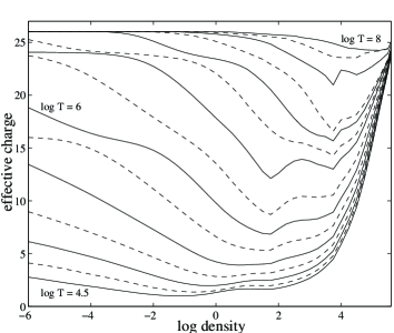
Fig. 1.: Isotherms of effective charge for Fe obtained from the interpolated EOS at log$T$[K] = 4.5 (solid line), 4.75 (dashes), 5 (solid), …8.

Figure1 shows the isotherms of $Z_{\rm eff}$ corresponding to the interpolated Fe EOS. The decreasing parts of the curves reflect the electron recombination due to the reduction of phase space per particle with increasing density. In this low-density region, our $Z_{\rm eff}$ coincides with $\langle Z\rangle$ given by the OPAL data (when available) within $\sim 10$%. The increase of $Z_{\rm eff}$ at high densities corresponds to pressure ionization. The non-monotonic behaviour at intermediate densities reflects consecutive pressure destruction of different electron shells of Fe atoms.

2.3 Opacities

2.3.1 Radiative opacities

In recent years, a significant progress has been made in calculations of the radiative opacities in dense atmospheres. We use the most recent OPAL opacity library (Rogers et al. 1996). For iron and hydrogen, it displays the tables of the spectral opacities, which we convert into the Rosseland opacities $K_{\rm rad}$ using the standard frequency-averaging procedure (e.g., Schwarzschild 1958). For helium, we implement the Rosseland opacities readily available in the OPAL library.

For $(\rho,T)$ values within the table range ($\rho<\rho_{\rm OPAL}$), we have used bilinear interpolation of $\log K_{\rm rad}$ between the table entries in $\log\rho$ and $\log T$. For $\rho>\rho_{\rm OPAL}$, we employ similar bilinear extrapolation based on the nearest pairs of table entries in $\log\rho$ and $\log T$. The extrapolated values of $K_{\rm rad}$ have practically no effect on temperature profiles, because at high densities the heat transport is provided by electrons ($K_{\rm c}\ll K_{\rm rad}$).

2.3.2 Conductive opacities

Previous studies of the temperature profiles in NS envelopes have mainly used the electron thermal conductivity of completely ionized, strongly degenerate plasma. In particular, one has often taken the conductive opacities from Urpin & Yakovlev (1980) and Yakovlev & Urpin (1980) (hereafter YU). However, in a cold enough NS, the thermal conductivity of non-degenerate or partly degenerate electrons may become important. A comparison with the tabular data of Hubbard & Lampe (1969) reveals that a straightforward extrapolation of the YU formulae from their validity domain (fully ionized, degenerate plasma) to the case of non-degenerate matter may lead to an underestimation of the electron thermal conductivity by orders of magnitude. As will be shown in Sect.3, this may strongly affect the temperature profiles in the NS envelopes at $T_{\rm eff}\mathrel{\mathchoice{\vbox{\offinterlineskip\halign{\hfil$\displaystyle#$\hfil\cr<\cr\sim\cr}}}{\vbox{\offinterlineskip\halign{\hfil$\textstyle#$\hfil\cr<\cr\sim\cr}}}{\vbox{\offinterlineskip\halign{\hfil$\scriptstyle#$\hfil\cr<\cr\sim\cr}}}{\vbox{\offinterlineskip\halign{\hfil$\scriptscriptstyle#$\hfil\cr<\cr\sim\cr}}}}10^{5}$K.

In order to determine the conductive opacities for any degeneracy, we employ the numerical code developed recently by Potekhin & Yakovlev (1996) (hereafter PY) for calculating the electron transport coefficients along magnetic fields in the magnetized NS envelopes. The code performs numerical thermal averaging of the effective energy-dependent electron relaxation time with the Fermi–Dirac distribution at any degeneracy. This enables us to consider not only strongly degenerate, but also mildly degenerate matter. In addition, PY have improved the approach of YU by a more accurate calculation of the Coulomb logarithm for the electron-ion scattering in the liquid phase of NS matter and by incorporating the Debye–Waller reduction factor (e.g., Itoh et al. 1984) for the electron-phonon scattering in the solid phase.

In the present article, we apply the above code for the particular case of zero magnetic field. For this purpose, further modifications have been made. First, in addition to the thermal conduction produced by the electron-ion scattering considered by PY, we have incorporated also the contribution from the electron-electron scattering in the liquid regime (see Sect.A.1). This process can be important for light elements (H, He) in a weakly degenerate matter. Second, we have improved the Coulomb logarithm which determines the collision rate of strongly degenerate electrons with ions (see Sect.2.3.3). Third, in the solid regime, we have used the new expression for the electron thermal conductivity, derived recently by Baiko & Yakovlev (1995). Note that at temperatures much lower than the melting temperatures, the Coulomb scattering of electrons by charged impurities may become important (e.g., YU). It depends on the impurity charge and, most important, on its number density $n_{\rm imp}$ which is generally unknown in the NS envelopes. We will present the results obtained for pure crystals ($n_{\rm imp}\to 0$). Our calculations including ⁵⁶Ni impurities in iron envelopes show that the electron-impurity scattering may affect the temperature profiles in the crusts of cooling NSs, whenever the impurity concentration is sufficiently high, $n_{\rm imp}\mathrel{\mathchoice{\vbox{\offinterlineskip\halign{\hfil$\displaystyle#$\hfil\cr>\cr\sim\cr}}}{\vbox{\offinterlineskip\halign{\hfil$\textstyle#$\hfil\cr>\cr\sim\cr}}}{\vbox{\offinterlineskip\halign{\hfil$\scriptstyle#$\hfil\cr>\cr\sim\cr}}}{\vbox{\offinterlineskip\halign{\hfil$\scriptscriptstyle#$\hfil\cr>\cr\sim\cr}}}}0.01\,n_{\rm i}$. Finally, in the non-degenerate layers, we have performed the thermal averaging introducing modifications into the effective width of the Landau levels which was used by PY to account for collisional and inelastic broadenings of the Landau levels in strongly degenerate matter. The effective width proposed by PY becomes inadequate in the non-degenerate regime, and we have switched it off by multiplying by the factor $(1+10T/T_{\rm F})^{-1}$.

A comparison of our thermal conductivities with the tables of Hubbard & Lampe (1969) (at $\rho\mathrel{\mathchoice{\vbox{\offinterlineskip\halign{\hfil$\displaystyle#$\hfil\cr<\cr\sim\cr}}}{\vbox{\offinterlineskip\halign{\hfil$\textstyle#$\hfil\cr<\cr\sim\cr}}}{\vbox{\offinterlineskip\halign{\hfil$\scriptstyle#$\hfil\cr<\cr\sim\cr}}}{\vbox{\offinterlineskip\halign{\hfil$\scriptscriptstyle#$\hfil\cr<\cr\sim\cr}}}}10^{5}$ g cm^-3, where the tables are adequate) shows maximum discrepancy up to 30% for carbon and up to 70% for lighter elements in the non-degenerate regime, and still smaller discrepancies in mildly and strongly degenerate matter. More accurate values of the Coulomb logarithm obtained in Sect.2.3.3 modify $K_{\rm c}$ by about 5–30%, which has only a little effect on the thermal structure of the envelope (see Sect.3).

2.3.3 Coulomb logarithm

The thermal conductivity $\kappa$ of degenerate electrons ($T<T_{\rm F}$) in a liquid or a gas of ions with mass and charge numbers $A$ and $Z$ can be written as

$$\kappa={\pi^{2}k_{\rm B}^{2}Tn_{\rm e}\over 3m_{\ast}\nu_{\rm e}},$$ (12)

where $m_{\ast}=m_{\rm e}\sqrt{1+x^{2}}$, $\nu_{\rm e}=\nu_{\rm ei}+\nu_{\rm ee}$ is the effective electron collision frequency, $\nu_{\rm ei}$ is determined by the Coulomb electron-ion collisions, and $\nu_{\rm ee}$ is determined by the electron-electron collisions. New calculations and fits of $\nu_{\rm ee}$ are presented in Sect.A.1. In this section, we examine $\nu_{\rm ei}$. It can be expressed as (e.g., YU)

$$\nu_{\rm ei}={4m_{\rm e}^{\ast}Ze^{4}L\over 3\pi\hbar^{3}},$$ (13)

where $L$ is the Coulomb logarithm to be evaluated. It is a slowly varying function of $\rho$ and $T$.

First consider a strongly coupled Coulomb liquid of ions, at $1\mathrel{\mathchoice{\vbox{\offinterlineskip\halign{\hfil$\displaystyle#$\hfil\cr<\cr\sim\cr}}}{\vbox{\offinterlineskip\halign{\hfil$\textstyle#$\hfil\cr<\cr\sim\cr}}}{\vbox{\offinterlineskip\halign{\hfil$\scriptstyle#$\hfil\cr<\cr\sim\cr}}}{\vbox{\offinterlineskip\halign{\hfil$\scriptscriptstyle#$\hfil\cr<\cr\sim\cr}}}}\Gamma\mathrel{\mathchoice{\vbox{\offinterlineskip\halign{\hfil$\displaystyle#$\hfil\cr<\cr\sim\cr}}}{\vbox{\offinterlineskip\halign{\hfil$\textstyle#$\hfil\cr<\cr\sim\cr}}}{\vbox{\offinterlineskip\halign{\hfil$\scriptstyle#$\hfil\cr<\cr\sim\cr}}}{\vbox{\offinterlineskip\halign{\hfil$\scriptscriptstyle#$\hfil\cr<\cr\sim\cr}}}}\Gamma_{\rm m}$, where $\Gamma_{\rm m}$ is the critical value of the ion coupling parameter $\Gamma$ at which a Coulomb crystal melts ($\Gamma_{\rm m}$ = 172, for a classical ion system, Nagara et al. 1987; the deviations from the classical melting curve due to the quantum corrections turn out to be small at $\rho<10^{10}$ g cm^-3 for carbon and heavier ions – see Chabrier 1993). In this case, one usually assumes that the screening of the electron-ion Coulomb interaction is static and produced by the ion-ion correlations. The screening is described by the ion-ion structure factor $S(q)$. Extensive calculations of $L$ in the Born approximation for different ion species, $Z$ and $A$, were performed by Itoh et al. (1983). The authors used the structure factors obtained in the approximation of rigid electron background. They fitted their results by complicated expressions. Later Yakovlev (1987) evaluated non-Born corrections to $L$, using the weak screening approximation.

Now we recalculate the Coulomb logarithm for strongly degenerate electrons at $1\mathrel{\mathchoice{\vbox{\offinterlineskip\halign{\hfil$\displaystyle#$\hfil\cr<\cr\sim\cr}}}{\vbox{\offinterlineskip\halign{\hfil$\textstyle#$\hfil\cr<\cr\sim\cr}}}{\vbox{\offinterlineskip\halign{\hfil$\scriptstyle#$\hfil\cr<\cr\sim\cr}}}{\vbox{\offinterlineskip\halign{\hfil$\scriptscriptstyle#$\hfil\cr<\cr\sim\cr}}}}\Gamma\mathrel{\mathchoice{\vbox{\offinterlineskip\halign{\hfil$\displaystyle#$\hfil\cr<\cr\sim\cr}}}{\vbox{\offinterlineskip\halign{\hfil$\textstyle#$\hfil\cr<\cr\sim\cr}}}{\vbox{\offinterlineskip\halign{\hfil$\scriptstyle#$\hfil\cr<\cr\sim\cr}}}{\vbox{\offinterlineskip\halign{\hfil$\scriptscriptstyle#$\hfil\cr<\cr\sim\cr}}}}\Gamma_{\rm m}$ from the expression

$$L=\int_{0}^{2k_{\rm F}}\,{\rm d}q\,{q^{3}S(q)F^{2}(q)R(q)\over q^{4}\epsilon(q)}\left(1-{\beta^{2}q^{2}\over 4k_{\rm F}^{2}}\right),$$ (14)

where $\beta=x/\sqrt{1+x^{2}}$, $k_{\rm F}=p_{\rm F}/\hbar$, $\hbar q$ is a momentum transfer in an $ei$ collision event, $\epsilon(q)$ is the static longitudinal dielectric function of electrons, $F(q)$ is the nuclear form factor to allow for finite nuclear size, and $R(q)$ is the non-Born correction factor specified below. The dielectric function has been calculated for the electron gas at any degeneracy. However, we have verified that, for all the cases in the present study, this dielectric function yields the same results as the function obtained in the limit of strong electron degeneracy for the relativistic electron gas (Jancovici 1962). Thus the bulk of the calculations has been done with this latter function. We use the nuclear form factor $F(q)$ appropriate to a uniform proton core of an atomic nucleus, with the same core radii as in Itoh et al. (1983). The finite sizes of the nuclei appear to have almost no effect on $L$, for the conditions of study. Nevertheless we have kept $F(q)$ in our calculations. Following Yakovlev (1987), the non-Born factor has been taken as $R(q)=\sigma(q)/\sigma_{\rm B}(q)$, where $\sigma(q)$ is the exact differential Coulomb scattering cross section for a momentum transfer $q$, and $\sigma_{\rm B}(q)$ is the cross section in the Born approximation. The exact cross sections are taken from Doggett & Spencer (1956).

In our calculations from Eq. (14), we have used the ion structure factors evaluated for a responsive electron background including the local field corrections between electrons (Chabrier 1990). Our calculations extend those of Itoh et al. (1983) by including the non-Born corrections and the effects of electron response on the ion structure factors. On the other hand, we improve the results of Yakovlev (1987) since we evaluate the non-Born corrections beyond the weak screening approximation.

We have evaluated $L$ from Eq. (14) for chemical elements with $1\leq Z\leq 26$ and for a dense grid of $1\leq\Gamma\leq\Gamma_{\rm m}$ and $10^{2}$ g cm${}^{-3}\leq\rho\leq 10^{10}$ g cm^-3 provided $T\leq T_{\rm F}$. In the case of hydrogen, we have restricted ourselves to $\rho\leq 10^{8}$ g cm^-3 since hydrogen should be completely burnt at higher densities. For light elements, the highest temperatures included in these data correspond to $\Gamma=1$ and appear to be much below $T_{\rm F}$. Accordingly, there exists a large temperature interval in the electron degeneracy domain where $\Gamma<1$, the ion coupling ceases to be strong, the ion screening cannot be treated in terms of ion-ion correlations, and Eq. (14) is invalid. In principle, the Coulomb logarithm for mildly-coupled ion plasma ($\Gamma\mathrel{\mathchoice{\vbox{\offinterlineskip\halign{\hfil$\displaystyle#$\hfil\cr<\cr\sim\cr}}}{\vbox{\offinterlineskip\halign{\hfil$\textstyle#$\hfil\cr<\cr\sim\cr}}}{\vbox{\offinterlineskip\halign{\hfil$\scriptstyle#$\hfil\cr<\cr\sim\cr}}}{\vbox{\offinterlineskip\halign{\hfil$\scriptscriptstyle#$\hfil\cr<\cr\sim\cr}}}}1$) can be evaluated using the formalism developed by Boerker et al. (1982). In order to simplify our analysis, we will restrict ourselves to the weak–coupling case ($\Gamma\ll 1$), in which the ions constitute a Boltzmann gas, the weak ion screening is dynamical and can be described by the dielectric function formalism, while the electron screening remains static (e.g., Lampe 1968). At $\Gamma\ll 1$ and $T<T_{\rm F}$, we propose the expression

$$L = {1\over 2}\ln\left({1\over b_{\rm i}}\right)-{1\over 2}\,\eta\ln\left({1\over\eta}\right)+{1\over 2}\,(1+\eta)\ln\left({1\over 1+\eta}\right)$$ (15)

$$- {1\over 2}\,\beta^{2}+{1\over 2}\,\pi Z\alpha\beta,$$

where $b_{\rm i}=1/(2k_{\rm F}r_{\rm Di})=1/\sqrt{3\Gamma}$ is the ion screening parameter in the weak coupling regime, $r_{\rm Di}$ is the Debye radius of ions, $\eta=b_{\rm e}/b_{\rm i}$, $b_{\rm e}=k_{\rm TF}/(2k_{\rm F})=\sqrt{\alpha/(\pi\beta)}$ is the electron screening parameter, $k_{\rm TF}$ being the inverse screening length of a charge by degenerate plasma electrons and $\alpha$ the fine-structure constant. The first three terms represent the Coulomb logarithm obtained for degenerate electrons and weakly coupled ions with the non-relativistic $ei$ scattering cross section. The expression presented is valid for $\eta<1$; it can be derived using the formalism of Williams & DeWitt (1969) to account for the dynamic ion screening and to integrate the $ei$ collision rate over velocities of ions. The fourth term is the relativistic correction in the weak–coupling limit (e.g., YU). The fifth term is the second–Born correction in the weak–coupling limit (Yakovlev 1987). Thus, we have supplemented our table of the Coulomb logarithms calculated for $\Gamma\geq 1$ (see above) with new values evaluated from Eq. (15) for $\Gamma<0.25$ and $T<T_{\rm F}$. Analytic fits to the full set of about 31,000 values of $L$ are presented in Sect.A.2. The tables of $L$ are freely available in the electronic form.

For illustration, in Fig. 2 (left panel) we compare the Coulomb logarithms in fully ionized Fe and C plasmas with those calculated in the Born approximation (Itoh et al. 1983). The non-Born corrections enhance the small–angle Coulomb scattering cross section, and increase $L$. The increase is especially pronounced for the heavier element, Fe (exceeds 20%), at densities $\rho\mathrel{\mathchoice{\vbox{\offinterlineskip\halign{\hfil$\displaystyle#$\hfil\cr>\cr\sim\cr}}}{\vbox{\offinterlineskip\halign{\hfil$\textstyle#$\hfil\cr>\cr\sim\cr}}}{\vbox{\offinterlineskip\halign{\hfil$\scriptstyle#$\hfil\cr>\cr\sim\cr}}}{\vbox{\offinterlineskip\halign{\hfil$\scriptscriptstyle#$\hfil\cr>\cr\sim\cr}}}}10^{6}$ g cm^-3, where the electrons are relativistic. The non-Born corrections become less important with decreasing $Z$, and they are negligible for light elements (H, He).

The inclusion of the electron response in the calculations of the ionic structure factors affects the Coulomb logarithm $L$ for H and He at $\Gamma\mathrel{\mathchoice{\vbox{\offinterlineskip\halign{\hfil$\displaystyle#$\hfil\cr>\cr\sim\cr}}}{\vbox{\offinterlineskip\halign{\hfil$\textstyle#$\hfil\cr>\cr\sim\cr}}}{\vbox{\offinterlineskip\halign{\hfil$\scriptstyle#$\hfil\cr>\cr\sim\cr}}}{\vbox{\offinterlineskip\halign{\hfil$\scriptscriptstyle#$\hfil\cr>\cr\sim\cr}}}}1$, as demonstrated on the right panel of Fig. 2. One can observe an increase of $L$ up to 15% for H at $\rho=10^{2}$ g cm^-2 and $\Gamma=10$ with respect to the case of rigid electron background. Actually, the increase grows with $\Gamma$ and reaches about 40% at $\Gamma=160$. The effect is weaker for He, and small for heavier elements (in the adopted parameter range). Thus, for the elements heavier than He, we have used the structure factors calculated in the rigid background approximation.

Note that calculated values of $L$ determine also the electric conductivity of degenerate matter in a liquid or gaseous ionic plasma, $\sigma=e^{2}n_{\rm e}/(m_{\rm e}^{\ast}\nu_{\rm ei})$.

Fig. 2.: Coulomb logarithm $L$ vs density for fully ionized plasmas at $\Gamma=10$. Left panel: Fe and C plasmas; dash-and-dots — present calculations, solid line — analytic fits (Sect.A.2), dashes — Born approximation (Itoh et al. 1983). Right panel: H and He plasmas; dots — present calculations, solid line — analytic fits, dash-and-dots — ion-structure factors in the rigid electron background (Itoh et al. 1983).

3 Results and discussion

3.1 Thermal structure of non-accreted envelopes

In this section, we consider a non-accreted NS envelope composed solely of iron, which may be at various ionization stages. We use the OPAL iron EOS where available, the ideal-gas EOS with the Coulomb correction (11) at high densities, and the interpolated EOS at intermediate densities as described in Sect.2.2.4. The conduction properties are described in the mean ion approximation with the effective ion charge $Z_{\rm eff}$ determined consistently with the EOS (Sect.2.2.5).

Fig. 3.: Boundary conditions for the thermal structure equation (1). Surface density is obtained from Eq.(5) as a function of surface temperature, for gravities $g_{14}$=0.4, 1, 2.43, 6. Dash-dotted lines correspond to a non-accreted matter (Fe opacities), and solid lines to an accreted matter (H opacities).

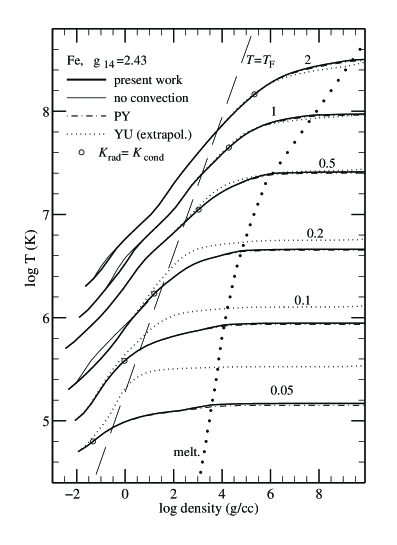
Fig. 4.: Temperature profiles in a non-accreted NS (heavy solid lines) compared with various approximations: after Yakovlev & Urpin (1980) (YU) by extrapolating the conductive opacities to $T>T_{\rm F}$; after Potekhin & Yakovlev (1996) (PY); and with neglected convection (thin solid lines). The curves are labeled by the values of $T_{\rm eff}/10^{6}\,{\rm K}$. Circles show the points, where the radiative opacity equals the conductive one; heavy dots show the melting curve $\Gamma=172$; long dashes display the degeneracy curve, $T=T_{\rm F}$.

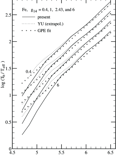
Fig. 5.: Temperature increase through non-accreted NS envelopes with different values of the surface gravity as compared to Eq.(16).

Figure 4 presents density dependence of the temperature in the NS envelope at various $T_{\rm eff}$. The integration of Eq.(1) has been started with the surface density $\rho_{\rm s}$, shown in Fig.3, and terminated at $\rho_{\rm b}=10^{10}$ g cm^-3. The value $g_{14}=2.43$ chosen in Fig.4 corresponds to a NS with a radius $R=10$ km and a mass $M=1.4\,M_{\odot}$. Circles on the curves are the points of equal radiative and conductive opacities. The thermal flux is mainly carried by radiation at lower densities and by electrons at higher densities. We also show the electron degeneracy curve and the melting curve.

In a wide range of $T_{\rm eff}$, some layers (Fig.4) turn out to be convectively unstable (Zavlin et al. 1996, Rajagopal & Romani 1996). In these layers, the energy transport is dominated by convection rather than by electron or radiative conduction. We describe the convective energy flux in the adiabatic approximation (Schwarzschild 1958), which assumes that the convective heat transport is much more efficient than other mechanisms. Accordingly, in the convective zones, we replace the temperature gradient given by Eq.(1) by the adiabatic gradient provided by the EOS tables.

In order to check the effect of convection, we have performed also calculations with “frozen” convection (i.e., neglecting the convection effect). This is the extreme case opposite to the adiabatic one. In this approximation, we obtain (Fig.4) slightly higher temperatures inside the convective part of the atmosphere. The atmospheric temperature profiles derived by Zavlin et al. (1996), who solved numerically the radiative transfer equation at moderate optical depths and described the convection using the mixing-length theory, lie between our two extremes. In deeper layers, the two extreme profiles tend to merge, as clearly seen in Fig.4. This merging occurs because the factor $K/T^{4}$ on the r.h.s. of Eq.(1) rapidly decreases, with increasing $T$, and thus ensures the isothermal profile at higher $T$ behind the convective zone (at fixed $T_{\rm eff}$). Thus, the thermal structure of the NS envelope at $\rho\mathrel{\mathchoice{\vbox{\offinterlineskip\halign{\hfil$\displaystyle#$\hfil\cr>\cr\sim\cr}}}{\vbox{\offinterlineskip\halign{\hfil$\textstyle#$\hfil\cr>\cr\sim\cr}}}{\vbox{\offinterlineskip\halign{\hfil$\scriptstyle#$\hfil\cr>\cr\sim\cr}}}{\vbox{\offinterlineskip\halign{\hfil$\scriptscriptstyle#$\hfil\cr>\cr\sim\cr}}}}10$ g cm^-3 is practically unaffected by the convection.

The dot-dashed curves in Fig.4 are obtained with $K_{\rm c}$ calculated according to PY (Sect. 2.3.2). These curves almost coincide with the solid lines, calculated more accurately. This confirms the validity of the PY approximations for the non-accreted envelopes.

If $T_{\rm eff}\mathrel{\mathchoice{\vbox{\offinterlineskip\halign{\hfil$\displaystyle#$\hfil\cr<\cr\sim\cr}}}{\vbox{\offinterlineskip\halign{\hfil$\textstyle#$\hfil\cr<\cr\sim\cr}}}{\vbox{\offinterlineskip\halign{\hfil$\scriptstyle#$\hfil\cr<\cr\sim\cr}}}{\vbox{\offinterlineskip\halign{\hfil$\scriptscriptstyle#$\hfil\cr<\cr\sim\cr}}}}2\times 10^{5}$K, the electron conduction becomes important not only in degenerate matter, but also in a non-degenerate region (Fig.4). Then the straight-line logarithmic extrapolation of the YU conductive opacities into the non-degenerate regions leads to a significant overestimation of the internal temperature (dotted curves).

This effect is seen also in Fig.5, that shows $\log(T_{\rm b}/T_{\rm eff})$ as a function of $\log T_{\rm eff}$ for four values of the surface gravity. If $\log T_{\rm s}\,[\mbox{K}]>5.5$, the well-known simple fit of GPE,

$$T_{\rm b6}=128.8\,(T_{\rm s6}^{4}/g_{14})^{0.455},$$ (16)

is rather accurate, but at lower $T_{\rm s}$ the deviations from this fit are quite pronounced. Nevertheless, the scaling law $T_{\rm b}=f(T_{\rm s}^{4}/g)$ holds with a good accuracy in the whole temperature–gravity range presented in this figure, except for the lowest $T_{\rm b}$ values. The fit which reproduces these new features is presented in Sect.A.3.

3.2 Thermal structure of accreted envelopes

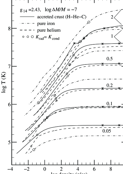
Fig. 6.: Temperature profiles in an accreted NS (solid lines) as compared to those in NS envelopes composed of pure iron (dot-dashed lines) and of pure helium (dashed line). The curves are labeled by $T_{\rm eff}/10^{6}\,{\rm K}$; full circles separate the regions of radiation and electron conduction; asterisks indicate the H/He (left) and He/C (right) interfaces.

The chemical composition of an accreted envelope depends on the composition of the infalling matter and on the nuclear transformations (thermo- or pycnonuclear burning, beta-captures) which occur while the matter sinks within the NS. The structure and stability of the accreted envelopes have been considered in number of works devoted to bursting NSs (see, e.g., Ayasli & Joss 1982, Paczyński 1983, Ergma 1986, Miralda-Escudé et al. 1990, Blaes et al. 1992, and references therein). However, most of the work focused either on high accretion rates or on slowly accreting old NSs whose internal temperature is solely determined by the accretion. On the contrary, we are mainly interested in not too old, cooling NSs with thin accreted envelopes, in which the heat release due to the nuclear transformations has no effect on the thermal structure.

Let us assume that an accreted envelope consists of shells with different chemical compositions. For an accretion of H/He, it is reasonable to expect that the outermost accreted layers are built of pure H, owing to the strong gravitational stratification (Alcock & Illarionov 1980), whereas He may exist in the deeper layers. The accretion is accompanied by the nuclear transformations of H/He into heavier elements. The details of these transformations are still uncertain, and we consider several models of accreted envelopes.

As a first example, we take the typical temperatures and densities of the nuclear burning from Ergma (1986) and assume the burning to be non-explosive. If $T_{\rm eff}$ is high and the accreted hydrogen layer reaches the region with $T\sim 4\times 10^{7}$K, then H burns efficiently into He in the thermonuclear regime. If temperature is lower and the hydrogen layer reaches the density $\rho\sim 10^{7}$ g cm^-3, a pycnonuclear burning of H into He proceeds. At higher $\rho\sim 10^{9}$ g cm^-3 and/or $T\sim 10^{8}$K, helium burns into carbon (Schramm et al. 1992). The pycnonuclear carbon burning occurs at $\rho\sim 10^{10}$ g cm^-3 (e.g., Yakovlev 1994), which is already inside the isothermal region of the envelope.

Figure 6 displays the thermal structure of a fully accreted envelope (the accreted mass $\Delta M\sim 10^{-7}M$ fills the layers up to $\rho\simeq\rho_{\rm b}$) of a NS with the surface gravity $g_{\rm s}=2.43\times 10^{14}$ cm s^-2. The outer, intermediate, and inner shells of this envelope, separated by asterisks, are composed of H, He, and C, respectively.

One can observe significant differences from the thermal structure of a non-accreted Fe envelope, as explained below. For a not too cold NS ($T_{\rm eff}\mathrel{\mathchoice{\vbox{\offinterlineskip\halign{\hfil$\displaystyle#$\hfil\cr>\cr\sim\cr}}}{\vbox{\offinterlineskip\halign{\hfil$\textstyle#$\hfil\cr>\cr\sim\cr}}}{\vbox{\offinterlineskip\halign{\hfil$\scriptstyle#$\hfil\cr>\cr\sim\cr}}}{\vbox{\offinterlineskip\halign{\hfil$\scriptscriptstyle#$\hfil\cr>\cr\sim\cr}}}}10^{5}$K), the main temperature gradient occurs in a layer of degenerate electron gas with ions in the liquid state, where the thermal conduction is mostly provided by the electrons due to the electron-ion collisions. The heavier the element, the smaller the thermal conductivity, and the steeper is the temperature growth inside the star. However, with decreasing $T_{\rm eff}$, the width of the heat–insulating degenerate layer becomes smaller, and the effect is less pronounced. In a cooler NS ($T_{\rm eff}\mathrel{\mathchoice{\vbox{\offinterlineskip\halign{\hfil$\displaystyle#$\hfil\cr<\cr\sim\cr}}}{\vbox{\offinterlineskip\halign{\hfil$\textstyle#$\hfil\cr<\cr\sim\cr}}}{\vbox{\offinterlineskip\halign{\hfil$\scriptstyle#$\hfil\cr<\cr\sim\cr}}}{\vbox{\offinterlineskip\halign{\hfil$\scriptscriptstyle#$\hfil\cr<\cr\sim\cr}}}}10^{5}$K), the main temperature gradient shifts into the NS atmosphere (to the optical depths $\sim 1$). For heavier elements, the atmospheric layers appear generally denser (at the same $T_{\rm eff}$, see Fig.3). Then the internal temperature gradient is weaker and the temperature grows slower inside the star. Thus, a not too cold accreted envelope is more heat–transparent than the iron envelope, whereas a cold accreted envelope is less heat-transparent. As seen from Fig. 3, the effective surface temperature which separates these two regimes is almost independent of the surface gravity.

Fig. 7.: Temperature increase through accreted NS envelopes for selected values of the surface gravity calculated using the full code (solid lines), PY-code (dot-dash lines), and PY-code supplemented by thermal conduction due to electron-electron collisions (dots).

Figure 7 demonstrates the effect of the improvements in the conductive opacities. The present results are compared with those in which the electron thermal conductivity is calculated with the PY code. Although the difference is not too large, it is higher than for the non-accreted Fe envelopes (Fig.4). The difference comes mostly from the electron-electron collisions (neglected in PY). Dots in Fig. 7 show the results obtained with the PY code supplemented by the contribution from the electron-electron collisions to the thermal conduction (Sect.A.1). The difference from the accurate results practically disappears.

Now let us analyze the sensitivity of the temperature profiles to the positions of the H/He and He/C interfaces. These interfaces, indicated by asterisks in Fig.6, are not well theoretically established. For example, the densities of nuclear H and He burning presented by Iben (1974) (see also Kippenhahn & Weigert 1990) are much lower than those given by Ergma (1986). We have significantly shifted the interfaces according to the results of Iben (1974), but the $T_{\rm eff}$–$T_{\rm b}$ relationship remains practically unchanged. We have also calculated the temperature profiles for a purely helium NS envelope. These profiles are slightly different from those in a burning accreted matter described above. However, the $T_{\rm eff}$–$T_{\rm b}$ relationships remain practically the same.

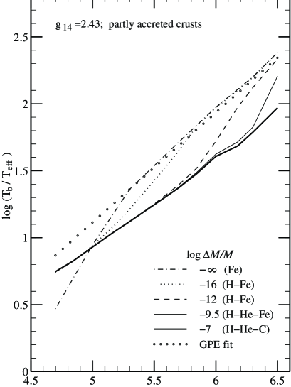
Fig. 8.: Temperature increase through partly accreted NS crusts.

Recently the thermal structure of old, slowly accreting NSs has been examined in several articles (see Miralda-Escudé et al. 1990, Blaes et al. 1992, and references therein). In these studies, the internal stellar temperature is assumed to be determined by the accretion rate. The composition of the accreted envelopes appears to be similar to the ones considered above except for the innermost layers. For instance, Miralda-Escudé et al. (1990) assume that He transforms directly into Fe while Blaes et al. (1992) state that the burning of He into C at $\rho\sim 10^{9}$ g cm^-3 is followed by the carbon transformation through the rapid ¹²C$(\alpha,\gamma)^{16}$O process. Accordingly, we have recalculated the temperature profiles replacing ¹²C by ⁵⁶Fe or ¹⁶O and found only very small differences. The insensitivity of the temperature profiles to the composition of the innermost layers of the envelope is quite natural, because these layers are nearly isothermal.

Summarizing the above discussion we can conclude that the $T_{\rm eff}$–$T_{\rm b}$ relationship is remarkably insensitive to the parameters of nuclear burning and to the chemical composition of accreted matter (H and/or He) but differs from the one in a non-accreted NS. This conclusion will not change if H burning is explosive (see, e.g., Paczyński 1983, Miralda-Escudé et al. 1990). During an outburst, the H-shell burns into He, without any noticeable effect on the $T_{\rm eff}$–$T_{\rm b}$ relation. According to Miralda-Escudé et al. (1990) helium burning in slowly accreting NSs is unstable; it produces nuclear outbursts with burning of all accreted material. Nevertheless, the helium layer should reach a very high density, $\rho\sim 10^{9}$ g cm^-3 to trigger the instability in a not too hot NS. If the same is true for the conditions of our interest, our results are valid during a long period of time until the instability is reached. However, according to Paczyński (1983), the presence of the heat outflow from a not too cold, cooling NS essentially stabilizes nuclear burning in accreted envelope, and the He burning is mostly non-explosive for the parameters we are interested in.

Figure8 shows $\log(T_{\rm b}/T_{\rm eff})$ as a function of $\log T_{\rm eff}$ for various amounts of accreted matter. The dot-dashed line represents $\log(T_{\rm b}/T_{\rm eff})$ for a non-accreted envelope from Fig.5. This function is strongly affected by the accretion. Even a thin hydrogen (or He) mantle of mass $\Delta M=10^{-16}M$, which extends only to $\rho\sim 10^{3}$ g cm^-3, modifies strongly the $T_{\rm b}$–$T_{\rm eff}$ relation. Analytical fits of $T_{\rm eff}$ as a function of the internal temperature $T_{\rm b}$, surface gravity $g$, and accreted mass $\Delta M$ are given in Sect.A.3.

3.3 Effect of accreted envelope on cooling

Consider briefly the effects of the possible presence of accreted matter in the NS envelopes on the thermal history of NSs. For this purpose, we simulate the cooling of NSs using two NS models. We use the cooling code of Gnedin & Yakovlev (1993) based on the approximation of isothermal NS interior. The code follows accurately the cooling of a not too young NS whose thermal relaxation is already over ($t\mathrel{\mathchoice{\vbox{\offinterlineskip\halign{\hfil$\displaystyle#$\hfil\cr>\cr\sim\cr}}}{\vbox{\offinterlineskip\halign{\hfil$\textstyle#$\hfil\cr>\cr\sim\cr}}}{\vbox{\offinterlineskip\halign{\hfil$\scriptstyle#$\hfil\cr>\cr\sim\cr}}}{\vbox{\offinterlineskip\halign{\hfil$\scriptscriptstyle#$\hfil\cr>\cr\sim\cr}}}}10^{2}$ yrs, see Nomoto & Tsuruta 1987, Umeda et al. 1994). We adopt a moderately stiff EOS of Prakash et al. (1988) to describe matter in the NS cores. This matter is assumed to consist of neutrons, protons, and electrons (no exotic cooling agents such as quarks or kaon condensates). The maximum NS mass, for this EOS, is about 1.7 $M_{\odot}$. We examine two NS models: (1) $M=1.30\,M_{\odot}$, $R=11.72$ km, the central density $\rho_{\rm c}=1.12\times 10^{15}$ g cm^-3; (2) $M=1.44\,M_{\odot}$, $R=11.35$ km, $\rho_{\rm c}=1.37\times 10^{15}$ g cm^-3.

The first model is a typical example of the standard cooling. The central density is insufficient to switch on the most powerful neutrino cooling due to the direct Urca process (Lattimer et al. 1991). In this case the main neutrino energy loss mechanisms in the NS cores are the modified Urca reactions (neutron and proton branches) and the nucleon-nucleon bremsstrahlung (Friman & Maxwell 1979, Yakovlev & Levenfish 1995).

Our second NS model is an example of the rapid neutrino cooling. In this model, the central density slightly exceeds the threshold density $\rho_{\rm cr}=1.30\times 10^{15}$ g cm^-3 of the direct Urca process (for the given EOS). Then the NS has a small central kernel (of radius 2.32 km and mass 0.035 $M_{\odot}$) where the direct Urca process operates, and the neutrino luminosity exceeds the standard one by several orders of magnitude.

All the neutrino energy loss rates included in the calculations are described by Levenfish & Yakovlev (1996). To simplify our analysis, we assume that the NS cores are non-superfluid, and there is no internal reheating (e.g., energy dissipation due to differential rotation). The results are presented in Fig. 9 in the form of the cooling curves – effective temperatures $T_{\rm eff}^{\infty}$ as measured by a distant observer (see Sect. 2.1) versus NS age $t$.

Figure 9 presents the cooling curves under the assumption that all the accreted material is accumulated at the NS surface during the NS birth. The accretion can occur, for instance, at the post-supernova stage (e.g., Chevalier 1989, 1996, Brown & Weingartner 1994) especially if the pulsar activity is suppressed initially by burying the pulsar magnetic field under the fallen-back matter (Muslimov & Page 1995). We show the standard and rapid neutrino cooling for different amount of accreted mass $\Delta M$. The fraction of accreted mass $\Delta M/M$ varies from 0 (non-accreted NSs) to $\sim 10^{-7}$ (fully accreted NS envelope). It is evident that further increase of $\Delta M$ does not affect the cooling.

The change of slopes of the cooling curves at $t=10^{5}$–$10^{6}$ yrs reflects the change of the cooling regime. Initially, a NS is at the neutrino cooling stage. It cools mainly via the neutrino emission; the internal stellar temperature is ruled by this emission and is thus independent of the thermal insulation of the NS envelope. The surface photon emission is determined by the $T_{\rm b}$–$T_{\rm eff}$ relation. Since the accreted envelopes of not too cold NSs are more thermally transparent (Sect. 3.2), the surface temperature of an accreted NS is noticeably higher than that of a non-accreted NS. One can see that even a very small fraction of accreted matter, such as $\Delta M/M\sim 10^{-16}$, may change appreciably the thermal history of the star. The colder the star, the smaller is the fraction of accreted material which yields the same cooling curve as the fully accreted NS envelope. The effect is naturally more pronounced for the rapid cooling (for colder NSs).

If $t\mathrel{\mathchoice{\vbox{\offinterlineskip\halign{\hfil$\displaystyle#$\hfil\cr>\cr\sim\cr}}}{\vbox{\offinterlineskip\halign{\hfil$\textstyle#$\hfil\cr>\cr\sim\cr}}}{\vbox{\offinterlineskip\halign{\hfil$\scriptstyle#$\hfil\cr>\cr\sim\cr}}}{\vbox{\offinterlineskip\halign{\hfil$\scriptscriptstyle#$\hfil\cr>\cr\sim\cr}}}}10^{5}$–$10^{6}$ yrs, the neutrino luminosity decreases, and the NS cools mainly via the surface emission of photons (the photon cooling stage). Since the envelopes of the accreting (and not too cold) NSs have lower thermal insulation, these stars cool now faster than the non-accreted ones (Fig. 9).

Fig. 9.: Standard and rapid cooling of NSs with non-accreted (Fe) and partly and fully accreted envelopes, compared with observations of thermal radiation from 6 pulsars (see text). The accreted mass is assumed to be accumulated during the first 100 yrs; numbers along the curves denote the values of $\log\Delta M/M$.

The change of the thermal history of a NS by the accreted material should be taken into account in theoretical interpretation of observational data on thermal radiation from NSs. For illustration, in Fig.9 we present the effective temperatures with $1\sigma$ confidence intervals of the pulsars 0833–45 Vela (Ögelman et al. 1993, Ögelman 1995), 0630+18 Geminga (Halpern & Ruderman 1993), 0656+14 and 1055–52 (Greiveldinger et al. 1996), RXJ 0002+6246 (Hailey & Craig 1995), and the $3\sigma$ upper limit for the Crab pulsar (PSR 0531+21, Becker & Aschenbach 1995). These data have been deduced from the fits of spectral observations of the ROSAT X-ray observatory. For Geminga, PSR 1055–52, and PSR 0656+14, we plot the values of $T_{\rm eff}$ obtained for “soft” components of the two- and three-component X-ray spectra models, since it is the soft component that is associated with the thermal flux from the stellar interior. For Vela, we extend downward the confidence interval obtained by Ögelman et al. (1993) according to the more recent spectral fitting of Ögelman (1995), that gives a more plausible NS radius than the previous fit.

The age of the Crab pulsar in Fig.9 is its true age known from the chronicles, the age of Vela is its possible true age determined recently by Lyne et al. (1996), the age of RXJ 0002+6246 is an estimate for the related supernova remnant G 117.7+06, while for the three other pulsars we adopt their characteristic ages.

We plot the values of $T_{\rm eff}$ derived by the authors by fitting the assumed blackbody thermal spectrum to the measured X-ray spectrum. The alternative often used is to derive $T_{\rm eff}$ from the apparent luminosity in the whole spectral range observed. However, this latter way is less certain, because the inferred temperature strongly depends on the assumed NS distance (usually poorly known) and model-dependent radius.

Note that the blackbody fits do not take into account the influence of the magnetized atmosphere. The fits for PSR 0656+14 (Anderson et al. 1993), Geminga (Meyer et al. 1994), and Vela (Page et al. 1996), which employ the models of magnetized atmospheres, have resulted in a few times lower $T_{\rm eff}$ than the blackbody models. Our justification of using here the blackbody data is that the so far developed models of magnetized atmospheres do not take proper account of absorption by neutral atoms. The neutral fraction can be significant at $T\sim 10^{5}-10^{6}$ K, because the magnetic fields $\sim 10^{12}$G increase the ground-state binding energy by about one order of magnitude. The opacities of hydrogen in such strong fields are still under investigation (see Pavlov & Potekhin (1995) and references therein).

The magnetic fields affect also the thermal insulation of the NS envelopes and, therefore, the cooling (e.g., Yakovlev & Kaminker 1994). We do not take this effect into account in the present article. As suggested by Hernquist (1985) and shown recently by Shibanov & Yakovlev (1996), the dipole surface magnetic fields $\mathrel{\mathchoice{\vbox{\offinterlineskip\halign{\hfil$\displaystyle#$\hfil\cr<\cr\sim\cr}}}{\vbox{\offinterlineskip\halign{\hfil$\textstyle#$\hfil\cr<\cr\sim\cr}}}{\vbox{\offinterlineskip\halign{\hfil$\scriptstyle#$\hfil\cr<\cr\sim\cr}}}{\vbox{\offinterlineskip\halign{\hfil$\scriptscriptstyle#$\hfil\cr<\cr\sim\cr}}}}3\times 10^{12}$G affect the cooling much more weakly than predicted by the studies of simplified magnetic field geometries (e.g., Van Riper 1988, 1991).

As seen from Fig. 9, for the pulsars Vela, Geminga, and RXJ 0002+6246, the presence of accreted matter would simplify the explanation of the cooling by the standard neutrino emission without invoking superfluidity of NS matter, as favoured in previous work (Page 1994, Levenfish & Yakovlev 1996). Interestingly, the accretion rate of Vela estimated by Morley (1996), multiplied by its age, yields $\log\Delta M/M_{\odot}\approx-9.5$, that just fits the middle of the error bar in Fig.9. For PSR 0656+14, the scenarios with and without the accretion are equally consistent with the result of the fitting shown if Fig.9, especially if we assume that its braking index is somewhat lower than 3 (as happens for all 4 pulsars with known braking indices, see Lyne et al. 1996) and therefore its true age is somewhat higher than its characteristic age. The relatively high temperature of PSR 1055–52 cannot be explained by the considered models of the cooling, that probably suggests some reheating process for this relatively old pulsar.

We have used, for illustration, the standard NS models and simplified blackbody fits to the observed spectra. More sophisticated models and fits can also gain from the assumption of accreted envelopes. For instance, Page (1996) considers the cooling of NSs with kaon condensed cores and reheating in the outer crusts, using our models of the envelopes.

4 Conclusions

We have considered thermal structure and evolution of NSs whose envelopes are composed of non-accreted or accreted matter. We have used new, state-of-the-art calculations of EOS and opacities of NS envelopes, described in Sect. 2. In particular, we have recalculated (Sects. 2.3.3, A.1, and A.2) the electron-electron and electron-ion collision frequencies, that determine the electron thermal conductivity, for a wide range of densities and temperatures of a degenerate electron gas and ionic liquid plasmas.

Using this new physics input, we have calculated (Sects. 3.1, 3.2) the temperature profiles in the envelopes of non-accreted and partly accreted NSs and obtained the relationships between the internal and effective temperatures of NSs, $T_{\rm b}$ and $T_{\rm eff}$. These relationships are important for simulating the NS cooling; they are fitted by simple analytic expressions in Sect.A.3. They appear to be very sensitive to the presence of accreted matter in the NS envelope; even a small amount of the accreted matter, $\Delta M\sim 10^{-16}\,M_{\odot}$, can reduce substantially the thermal insulation of the envelopes. For a non-accreting NS, our relationship between $T_{\rm b}$ and $T_{\rm eff}$ extends the well–known result of GPE to lower temperatures (down to $T_{\rm eff}\sim 50\,000$ K).

In Sect. 3.3, we have examined briefly the effect of the possible presence of accreted matter on the NS cooling. We show that the accreted matter may increase the surface temperature (photon thermal luminosity) at the neutrino cooling stage, and decrease them at the subsequent photon cooling stage, as compared to the NSs without accreted envelopes. We have shown that these results can be important for a proper interpretation of observed thermal radiation from NSs. In particular, the presence of accreted matter facilitates the explanation of recent observational results concerning the pulsars Vela and Geminga, and RXJ 0002+6246, in the framework of the standard neutrino emission model (without exotic matter, superfluidity, or direct Urca processes).

In this paper, we have neglected effects of magnetic fields on the EOS and the thermal conduction of matter, which can be significant (e.g., Yakovlev & Kaminker 1994). They do deserve further studies using improved EOS and thermal conductivities of magnetized NS envelope (e.g., PY) and improved radiative opacities of magnetized NS atmosphere (e.g., Pavlov & Potekhin 1995), with allowance for the possible presence of light elements in the surface layers.

Finally, it is worth noting that the physics input used in the present calculations can be applied to a variety of other astrophysical problems concerning dense stellar matter, e.g. the thermal structure and bursting activity of X-ray bursters (see, e.g., Miralda-Escudé et al. 1990 and references therein) and the cooling of white dwarfs (Segretain et al. 1994).

• We are grateful to H. DeWitt for pointing out the article of Boerker et al. (1982), to Dany Page and Yu.A. Shibanov for fruitful discussions, and to D. Page for reading the manuscript and making the most useful critical remarks. This work was supported in part by the RBRF grant No. 96-02-16870a, INTAS grant No. 94-3834, and DFG–RBRF grant No. 96-02-00177G. AYP gratefully acknowledges the hospitality of the theoretical astrophysics group of the Ecole Normale Supérieure de Lyon.

Appendix: fitting formulae

A.1 Electron-electron collisions

The effective collision frequency $\nu_{\rm ee}$ of non-relativistic degenerate electrons ($x\ll 1$, $T<T_{\rm F}$) was analyzed by Lampe (1968) using the formalism of the dynamic screening of the electron–electron interaction. The expression of $\nu_{\rm ee}$ for the relativistic degenerate electrons at $T\ll T_{\rm pe}$ was obtained by Flowers & Itoh (1976). Here, $T_{\rm pe}$ is the electron plasma temperature determined by the electron plasma frequency $\omega_{\rm pe}$,

$$T_{\rm pe}={\hbar\omega_{\rm pe}/k_{\rm B}},\;\;\;\omega_{\rm pe}=\sqrt{{4\pi e^{2}n_{\rm e}/m_{\rm e}^{\ast}}},$$ (A1)

$m_{\rm e}^{\ast}=m_{\rm e}\sqrt{1+x^{2}}$. The degeneracy temperature $T_{\rm F}$ in the NS envelopes is typically higher than $T_{\rm pe}$. Urpin & Yakovlev (1980) extended the results of Flowers & Itoh (1976) to higher temperatures, $T<T_{\rm F}$. In the approximation of static electron screening of the Coulomb interaction, Urpin & Yakovlev (1980) obtained

$$\nu_{\rm ee}={3\alpha^{2}\,(k_{\rm B}T)^{2}\over 2\pi^{3}\,\hbar m_{\rm e}^{\ast}c^{2}\,b_{\rm e}^{3/2}}\,J(y),$$ (A2)

where $y=\sqrt{3}\,T_{\rm pe}/T$, $\alpha=e^{2}/(\hbar c)$, $\beta=x/\sqrt{1+x^{2}}$ and $b_{\rm e}=\alpha/(\pi\beta)$ (see Eq. (15)). Now it is sufficient to calculate the function $J(y)$, presented by Urpin and Yakovlev (1980) as a 2D integral which depends parametrically on the relativistic parameter $x$. Lampe (1968) analyzed this function in the static screening approximation at $x\ll 1$. The asymptotes of $J$ were obtained by Lampe (1968) for $x\ll 1$ at $y\ll 1$ and $y\gg 1$, by Flowers & Itoh (1976) for $y\gg 1$ at any $x$, and by Urpin & Yakovlev (1980) for $y\ll 1$ and $x\gg 1$. Timmes (1992) calculated $J(y)$ numerically in the limit of $x\gg 1$. However, the unified expression of $J(y)$ at $T<T_{\rm F}$ valid equally for relativistic and non-relativistic electrons has been absent. Note that the fit expression of $J(y)$ obtained by Timmes (1992) (his Eq.(10)) is valid only at $y<10^{3}$.

We have calculated $J$ numerically for a dense grid of $x$ and $y$ in the intervals $0.01\leq x\leq 100$ and $0.1\leq y\leq 100$. The results are fitted by the expression:

$$J = \left(1+{6\over 5x^{2}}+{2\over 5x^{4}}\right)\,\left[{y^{3}\over 3(1+0.07414\,y)^{3}}\right.$$ (A3)

$$\times \left.\ln\left({2.810-0.810\beta^{2}+y\over y}\right)+{\pi^{5}\over 6}\,{y^{4}\over(13.91+y)^{4}}\right]$$

which reproduces also all the asymptotic limits mentioned above. The mean error of the fits is 3.7%, and the maximum error of 11% takes place at $x=1$ and $y=0.1$.

A.2 Coulomb logarithms

The tables of the Coulomb logarithms calculated from Eqs. (14) and (15) as described in Sect. 2.3.3 are fitted by

$$L = {1\over 2}\,(1+c_{5}\,b)\ln\left({1+c_{7}b_{\rm e}\over b}\right)-c_{4}$$ (A4)

$$- {1\over 2}\,\beta^{2}(1-c_{6}b)+{1\over 2}\pi Z{\alpha\beta},$$

where $b=b_{\rm e}+b_{\rm i}$ and

$$b_{\rm i}=\left({3\over 2\pi Z}\right)^{2/3}\left(1.5c_{1}+{c_{3}\sqrt{Z}+c_{2}\beta^{2}\over\sqrt{\Gamma Z}}+{3\over\Gamma}\right)^{-1}.$$

For $Z\leq 3$, the fit parameters are given by:
$c_{1}=-0.349+1.766\,Z-0.413\,Z^{2}$,
$c_{2}=3.499-2.355\,Z+0.871\,Z^{2}$,
$c_{3}=11.92-6.77\,Z+1.04\,Z^{2}$,
$c_{4}=0.5733-0.1116\,Z+0.0159\,Z^{2}$,
$c_{5}=0.7060-0.9896\,Z+0.3517\,Z^{2}$,
$c_{6}=4.779-2.676\,Z+0.361\,Z^{2}$,
$c_{7}=2.457+2.523\,Z-1.014\,Z^{2}$.

For $Z>3$, we obtain $c_{1}=1.232$, $c_{2}=4.273$, $c_{3}=0.9742$, $c_{4}=0.3816$ $c_{5}=0.9025$, $c_{6}=0.0$, $c_{7}=0.9$.

If $Z=1$, the rms fit error over all our data set is about $\delta_{\rm av}\approx$ 3.2%, and the maximum error of $\delta_{\rm max}\approx$ 7.2% takes place at $\rho\approx 10^{5}$ g cm^-3 and $\Gamma=3$. If $Z=2$ we have $\delta_{\rm av}\approx$ 3.7%, $\delta_{\rm max}\approx$ 7.8% at $\rho\approx 10^{9}$ g cm^-3 and $\Gamma=1$. For $Z=3$, we obtain $\delta_{\rm av}\approx$ 2.4%, $\delta_{\rm max}\approx$ 7.0% at $\log(\rho[{\rm g\;cm}^{-3}])\approx 2.5$ and $\Gamma=1$. For higher $Z$, the rms error remains about 1.5–1.7%, and the maximum error mainly decreases. For instance, we have $\delta_{\rm max}\approx$ 5.1% at $\log\rho\approx 2.25$ and $\Gamma=4$ for $Z=6$; $\delta_{\rm max}\approx$ 3.7% at $\log\rho\approx 5.75$ and $\Gamma=2$ for $Z=12$; and $\delta_{\rm max}\approx$ 3.4% at $\log\rho\approx 5.5$ and $\Gamma=8$ for $Z=26$. This fit accuracy is quite sufficient for studying the thermal structure of NSs.

A.3 Relation between internal and effective temperatures

In this section, we derive a fitting formula for $T_{\rm eff}$ as a function of $T_{\rm b}$, valid for $4.7\leq\log T_{\rm eff}\leq 6.5$, $0.4\leq g_{14}\leq 6$, where $g_{14}$ is the surface gravity in units of $10^{14}$ cm s^-2.

Let us define $T_{\rm b9}=T_{\rm b}/10^{9}$K, $T_{\rm eff6}=T_{\rm eff}/10^{6}$K, and

$$\eta\equiv g_{14}^{2}\Delta M/M,$$ (A5)

where $M$ is the NS mass and $\Delta M$ is the accreted mass. According to GPE, $\eta=P_{\rm b}/(1.193\times 10^{22}\mbox{ Mbar}),$ where $P_{\rm b}$ is the pressure at the bottom of the accreted envelope.

For a purely iron (non-accreted) envelope, a very crude estimate (with an error $\sim$ 30%) yields

$$T_{\rm eff6}=T_{\ast}\equiv\left(7\,T_{\rm b9}\sqrt{g_{14}}\right)^{1/2}.$$ (A6)

Then $\zeta\equiv T_{\rm b9}-(T_{\ast}/10^{3})$ is approximately an increase of the temperature through the iron envelope (in $10^{9}$K). A more accurate fitting formula reads

$$T_{\rm eff6,Fe}^{4}=g_{14}\,[(7\zeta)^{2.25}+(\zeta/3)^{1.25}].$$ (A7)

The typical fit error of $T_{\rm eff6,Fe}$ is about 2%, with maximum 4.2%, over the $T_{\rm eff}-g$ domain indicated above.

For a fully accreted envelope, we obtain

$$T_{\rm eff6,a}^{4}=g_{14}\,(18.1\,T_{\rm b9})^{2.42},$$ (A8)

which is valid at not too high temperature ($T_{\rm b}\leq 10^{8}$K).

Finally, for the partially accreted envelopes at any temperatures within the indicated range, we have

$$T_{\rm eff6}^{4}={a\,T_{\rm eff6,Fe}^{4}+T_{\rm eff6,a}^{4}\over a+1},$$ (A9)

where

$$a=\left[1.2+(5.3\times 10^{-6}/\eta)^{0.38}\right]\,T_{\rm b9}^{5/3}.$$ (A10)

The typical fit error of Eq. (A9) for $T_{\rm eff6}$ is about 3%, with maximum 5.2%, for all possible values of $\eta$ and any values of $g$ and $T_{\rm eff}$ within the indicated range.

The dependence (A7) is recovered not only at sufficiently low accreted mass ($\eta\to 0$), but also at sufficiently high $T_{\rm b}$. The latter result reflects the fact (first demonstrated by GPE) that at high $T_{\rm eff}$ the thermal insulation is mostly produced by the conductive opacities in the deep and hot layers of the envelope, in which light elements (H, He) burn into heavier ones. On the other hand, even at very low accreted mass ($\log\Delta M/M\sim-16$), the approximation of fully accreted crust is good enough at sufficiently low temperature because in this case the thermal insulation is provided mainly by the low-density accreted surface layers.

References

- 1 Alcock C., Illarionov A.F., 1980, ApJ 235, 534
- 2 Anderson S.B., Córdova F.A., Pavlov G.G., Robinson C.R., Thompson R.J., 1993, ApJ 414, 867
- 3 Ayasli S., Joss P.C., 1982, ApJ 256, 637
- 4 Baiko D.A., Yakovlev D.G., 1995, Astron. Lett. 21, 702.
- 5 Becker W., Aschenbach B., 1995, ROSAT HRI Observations of the Crab Pulsar. In: Alpar M.A., Kiziloğlu Ü., Paradijs J. van (eds.) The Lives of the Neutron Stars. Kluwer, Dordrecht, p. 47
- 6 Bignami G.F., Caraveo P.A., Mignani R., Edelstein J., Bowyer S., 1996, ApJ 456, L111
- 7 Blaes O.M., Blandford R.D., Madau P., Yan L., 1992, ApJ 399, 634
- 8 Boerker D.B., Rogers F.J., DeWitt H.E., 1982, Phys. Rev. A 25, 1623
- 9 Brown G.E., Weingartner J.C., 1994, ApJ 436, 843
- 10 Chabrier G., 1990, Journal de Physique 51, 57
- 11 Chabrier G., 1993, ApJ 414, 695
- 12 Chabrier G., Schatzman E. (eds), 1994, Proc. IAU Coll. 147, The Equation of State in Astrophysics. Cambridge Univ. Press, Cambridge
- 13 Chevalier R.A., 1989, ApJ 346, 847
- 14 Chevalier R.A., 1996, ApJ 459, 322
- 15 DeWitt H.E., Slattery W.L., Chabrier G., 1996, Physica B, 228, 21
- 16 Doggett J.A., Spencer L.V., 1956, Phys. Rev. 103, 1597
- 17 Ebeling W., Kraeft W.D., Kremp D., 1977, Theory of Bound States and Ionization Equilibrium of Plasmas and Solids. Akademie, Berlin
- 18 Ergma E., 1986, Sov. Sci. Rev. E: Astrophys. Space Phys. 5, 181
- 19 Fletcher C.A.J., 1988, Computational Techniques for Fluid Dynamics. Springer, Berlin
- 20 Flowers E., Itoh N., 1976, ApJ 206, 218
- 21 Fontaine G., Graboske H.C., Van Horn H.M., 1977, ApJS 35, 293
- 22 Friman B.L., Maxwell O.V., 1979, ApJ 232, 541
- 23 Gnedin O.Y., Yakovlev D.G., 1993, Astron. Lett. 19, 104.
- 24 Greiveldinger C., Camerini U., Fry W. et al., 1996, ApJ 465, L35
- 25 Gudmundsson E.H., Pethick C.J., Epstein R.I., 1983, ApJ 272, 286 (GPE)
- 26 Hailey C.J., Craig W.W., 1995, ApJ 455, L151
- 27 Halpern J.P., Ruderman M., 1993, ApJ 415, 286
- 28 Hansen J.-P., Vieillefosse P., 1975, Phys. Lett. A 53, 187
- 29 Hernquist L., 1984, ApJS 56, 325
- 30 Hernquist L., 1985, MNRAS 213, 313
- 31 Hernquist L., Applegate J.H., 1984, ApJ 287, 244
- 32 Huebner W.F., Merts A.L., Magee N.H., Argo M.F., 1977, Astrophysical Opacity Library. Rept. LA 6760M, Los Alamos Scientific Laboratory (LAO)
- 33 Hubbard W.B., Lampe M., 1969, ApJS 18, 297
- 34 Iben I., 1974, ARA&A 12, 215
- 35 Itoh N., Mitake S., Iyetomi H., Ichimaru S., 1983, ApJ 273, 774
- 36 Itoh N., Kohyama Y., Matsumoto N., Seki M., 1984, ApJ 285, 758; erratum 404, 418
- 37 Jancovici B., 1962, Nuovo Cimento 25, 428
- 38 Kippenhahn R., Weigert A., 1990, Stellar Structure and Evolution. Springer, Berlin
- 39 Lampe M., 1968, Phys. Rev. 170, 306
- 40 Landau L.D., Lifshitz E.M., 1986, Statistical Physics, Part I. Pergamon, Oxford
- 41 Lattimer J.M., Pethick C.J., Prakash M., Haensel P., 1991, Phys. Rev. Lett. 66, 2701
- 42 Levenfish K.P., Yakovlev D.G., 1996, Astron. Lett. 22, 56
- 43 Lyne A.G., Pritchard R.S., Graham-Smith F., Camilo F., 1996, Nature 381, 497
- 44 Meyer R., Pavlov G.G., Mészáros P., 1994, ApJ 433, 265
- 45 Miralda-Escudé J., Haensel P., Paczyński B., 1990, ApJ 362, 572
- 46 Morley P.D., 1996, A&A 313, 204
- 47 Muslimov A., Page D., 1995, ApJ 440, L77
- 48 Nagara H., Nagata Y., Nakamura T., 1987, Phys. Rev. A36, 1859
- 49 Nelson R.W., Salpeter E.E., Wasserman I., 1993, ApJ 418, 874
- 50 Nomoto K., Tsuruta S., 1987, ApJ 312, 711
- 51 Ögelman H., Finley J.P., Zimmermann H., 1993, Nature 361, 136
- 52 Ögelman H., 1995, X-ray Observations of Cooling Neutron Stars. In: Alpar M.A., Kiziloğlu Ü., Paradijs J. van (eds.) The Lives of the Neutron Stars. Kluwer, Dordrecht, p. 101
- 53 Paczyński B., 1983, ApJ 264, 282
- 54 Page D., 1994, ApJ 428, 250
- 55 Page D., 1996, ApJ Lett. (submitted)
- 56 Page D., Shibanov Yu.A., Zavlin V.E. 1996, Temperature, Distance and Cooling of the Vela Pulsar. In: Zimmermann H.-U., Trümper J., Yorke H. (eds) Proc. Int. Conf. on X-ray Astronomy and Astrophysics, Röntgenstrahlung from the Universe. MPE Report 263, Garching, p. 173
- 57 Pavlov G.G., Potekhin A.Y., 1995, ApJ 450, 883
- 58 Potekhin A.Y., 1996, Physics of Plasmas (in press)
- 59 Potekhin A.Y., Yakovlev D.G., 1996, A&A 314, 341 (PY).
- 60 Prakash M., Ainsworth T.L., Lattimer J.M., 1988, Phys. Rev. Lett. 61, 2518
- 61 Rajagopal M., Romani R.W., 1996, ApJ 461, 327
- 62 Rogers F.J., Swenson F.J., Iglesias C.A., 1996, ApJ 456, 902
- 63 Saumon D., Chabrier G., Van Horn H.M., 1995, ApJS 99, 713 (SCVH)
- 64 Schaaf M.E., 1988, A&A 205, 335
- 65 Schaaf M.E., 1990, A&A 235, 499
- 66 Schramm S., Langanke K., Koonin S.E., 1992, ApJ 397, 579
- 67 Schwarzschild M., 1958, Structure and Evolution of the Stars. Princeton Univ. Press, Princeton
- 68 Segretain L., Chabrier G., Hernanz M., et al., 1994, ApJ 434, 641
- 69 Shibanov Yu.A., Yakovlev D.G., 1996, A&A 309, 171
- 70 Stringfellow G.S., DeWitt H.E., Slattery W.L., 1990, Phys. Rev. A 41, 1105
- 71 Thorne K.S., 1977, ApJ 212, 825
- 72 Timmes F.X., 1992, ApJ 390, L107
- 73 Umeda H., Tsuruta S., Nomoto K., 1994, ApJ 433, 256
- 74 Urpin V.A., Yakovlev D.G., 1980, SvA 24, 126
- 75 Van Riper K.A., 1988, ApJ 329, 339
- 76 Van Riper K.A., 1991, ApJS 75, 449
- 77 Williams R.H., DeWitt H.E., 1969, Phys. Fluids 12, 2326
- 78 Yakovlev D.G., 1987, SvA 31, 347
- 79 Yakovlev D.G., 1994, Acta Phys. Polonica 25B, 401
- 80 Yakovlev D.G., Kaminker A.D., 1994, Neutron Star Crusts with Magnetic Fields. In: Chabrier G., Schatzman E. (eds) Proc. IAU Coll. 147, The Equation of State in Astrophysics. Cambridge Univ. Press, Cambridge, p. 214
- 81 Yakovlev D.G., Levenfish K.P., 1995, A&A 297, 717
- 82 Yakovlev D.G., Shalybkov D.A., 1989, Sov. Sci. Rev. E: Astrophys. Space Phys. 7, 313
- 83 Yakovlev D.G., Urpin V.A., 1980, SvA 24, 303 (YU)
- 84 Zavlin V.E., Pavlov G.G., Shibanov Yu.A., Rogers F.J., Iglesias C.A., 1996, X-ray Spectra from Convective Photospheres of Neutron Stars. In: Zimmermann H.-U., Trümper J., Yorke H. (eds) Proc. Int. Conf. on X-ray Astronomy and Astrophysics, Röntgenstrahlung from the Universe. MPE Report 263, Garching, p. 209