The age of the most nearby star

Abstract

We address the question how accurately stellar ages can be determined by stellar evolution theory. We select the star with the best observational material available - our Sun. We determine the solar age by fitting solar evolution models to a number of observational quantities including several obtained from helioseismology, such as photospheric helium abundance or p-mode frequencies. Different cases with respect to the number of free parameters and that of the observables to be fitted are investigated. Age is one of the free parameters determined by the procedure. We find that the neglect of hydrogen-helium-diffusion leads to ages deviating by up to 100% from the true, meteoritic solar age. Our best models including diffusion yield ages by about 10% too high. The implication for general stellar age determination is that a higher accuracy than that can not be expected, even with the most up-to-date models. Our results also confirm that diffusion as treated presently in solar models is slightly too effective.

Key words: Sun: evolution, interior – Stars: evolution, interior

1 Introduction

Stellar evolution theory is able to derive the age of stars or stellar systems from a few basic observational data and therefore can provide constraints on the evolution of galaxies and the universe itself. Recently, it has become evident that improvements in the input physics used for the stellar model calculations lead to considerably reduced ages for Pop.II stars as observed in globular clusters (Chaboyer & Kim 1995; Mazzitelli et al.1995; Salaris et al.1997), thereby bringing into consistency globular cluster ages and cosmic expansion ages. In this context, the question of the accuracy of stellar age determinations arises. The errors given for globular cluster ages reflect the observational uncertainties only, while those of the stellar models are usually ignored. Chaboyer (1995) and Shi (1995) have investigated the influence of various physical assumptions on ages determined from the main sequence turn-off and found possible variations of up to order 10%. One of these – the inclusion of non-ideal effects in the equation of state – resulted in the reduced cluster ages.

The influence of the model errors on the derived ages depend, of course, on the dating method used. One therefore tries to find ways to minimize the influence of possible sources of error or to determine relative ages, which in general are more accurate. For a discussion of several methods for globular clusters, see Stetson et al.(1996). In general, the predicted colour and/or visual brightness of the turn-off as a function of age is the decisive quantity, although differential age determinators using the colour or brightness difference between the turn-off and some time-independent cluster-diagram feature are being used to minimize the influence of systematic offsets.

A completely independent method to determine stellar ages is used for eclipsing binary systems. One can, for example, try to match the positions in the Hertzsprung-Russell- or Colour-Magnitude-Diagram of both components of known mass with stellar evolution tracks. A necessary condition for a credible age-determination is then that the two error boxes are hit for the same age along both tracks. The classical example for such a successful age determination is AIPhe (Andersen et al.1988) with determined ages that agree better than 10%. Schröder et al. (1997) recently have investigated $\zeta$Aur systems in a different, but related context. In the future, detached eclipsing binary systems detected in massive photometric searches (e.g. Kaluzny et al.1996) will allow to determine globular cluster ages much more directly (see Paczyński 1996a for a review). For that purpose, theoretical luminosity–age–relations for a variety of stellar masses and compositions will be necessary (Weiss & Schlattl 1997) that will yield the age (and possibly the helium content; cf.  Paczyńksi 1996a) of cluster stars of known mass, metallicity and luminosity. Again, the question will be: how accurate are such age determinations in terms of the theoretical uncertainties?

To answer this and other questions concerning the accuracy of stellar ages, Paczyńksi (1996b) suggested to investigate how accurate we can determine the age of the best-known star - our Sun. In calculating solar models, the solar age as determined from meteorites usually is one of the parameters to be fitted by the model. Along with luminosity, effective temperature and the metal-to-hydrogen ratio $Z/X$ it determines the model parameters (initial helium content; mixing-length parameter); the solar model then provides predictions for the neutrino fluxes, p-mode frequencies and other quantities. Since the agreement between models and solar properties determined from helioseismological observations is very good, this is implicitely taken as evidence that the solar age is appropriate for the models. However, there are indications that a slightly different age might lead to even better agreement. Dziembowski et al. (1994) have investigated a solar seismic model of only 4 billion years. Although they exclude this model, they also state that a much smaller change in age $(\pm 5\cdot 10^{7}$ years) cannot be ruled out by helioseismology. Schlattl et al. (1997) find that their solar model would agree better with observations, if the solar age would be raised.

In the present paper, we will turn around the standard solar model approach. A set of observables will be given which the models have to match. The solar age will now be a quantity resulting from the best fit to the observables. That way, we will be able to determine the solar age from stellar models. The comparison with the meteoritic “true” age will give us indications how accurate stellar ages can be determined for the case of the most precisely known stellar parameters. For any other star, the accuracy will be lower. It will also define the best set of input physics assumptions able to yield the most accurate ages. Since the solar mass and luminosity are among the known parameters, the solar case is a stringent test case for age determinations of globular clusters based on detached eclipsing binaries.

In the next section we will shortly review the numerical code and the input physics assumptions of our solar model calculations published in Schlattl et al. (1997). Section3 will present solar age determinations based on fits to different sets of solar quantities, among them interior sound speed and p-mode frequencies. The final section will contain our conclusions.

2 The solar model calculations

For the present work, we have used the same solar model code as described in Schlattl et al. (1997). Here, we merely recall its basic features and input physics details.

The opacities are combinations of the OPAL-tables (Rogers & Iglesias 1992; Iglesias & Rogers 1996) with either those of Weiss et al. (1990) or Alexander & Fergusson (1994) for the low-temperature regime. For the EOS we either use a Saha-type equation or the OPAL equation of state (Rogers et al. 1996). If diffusion is included, the diffusion coefficients are calculated according to Thoul et al. (1994). For this work, only hydrogen-helium-diffusion has been taken into account. For the layers above $\tau\approx 20$ model atmospheres have been used for the calculations of the p-mode frequencies and as the outer boundary condition for the inner model. Since the model atmospheres extend into the convective envelope and take into account convection according to the mixing-length description with a parameter $\alpha_{\rm at}=0.5$, no constant value for the mixing-length parameter $\alpha_{\rm int}$ can be used. Rather, a smooth transition has been achieved by using the function

$$\alpha(T) = f(T)\times\alpha_{\rm int}+\left(1-f(T)\right)\times\alpha_{\rm at}$$

$$\rm where$$

$$f(T) = \left(1+\exp\left(\frac{T_{0}-T}{\Delta T}\right)\right)^{-1}$$ (1)

and the parameters $T_{0}$ and $\Delta T$ being 10 800 resp. 180 K. $\alpha_{\rm int}$ remains the parameter to be determined by the solar model and replaces the global value $\alpha_{\rm MLT}$ used in models with standard grey atmospheres. The calculations of Sect.3.1 were performed with those standard atmospheres and a constant $\alpha_{\rm MLT}$.

The composition changes due to nuclear reactions are calculated using a network incorporating the p-p and CNO-cycle using the same reaction rates as in Castellani et al. (1994). The calculations are started on the pre-main sequence with a homogeneous model powered by gravothermal energy only. Both the spatial and temporal resolution are checked for their accuracy and therefore allow a controlled precision of the models. For further details the reader is refered to Schlattl et al. (1997).

Table1 lists the solar values adopted and the references for the quantities resulting from helioseismological observations and inversions.

Table 1.: Solar values adopted in this paper and references for quantities inferred from helioseismology. _⊙ denotes the present Sun. $Y_{\odot}$ is the present surface helium content and $R_{\rm cz}$ the radius of the convective envelope’s lower boundary. $\nu$ indicates symbolically p-mode frequencies and $u$ the isothermal sound speed. All other symbols have their usual meaning. Errors are $1\sigma$ errors as given in the original papers. The references are: (1) Grevesse & Noels (1993); (2) Dziembowski et al.(1994); (3) Basu et al.(1996); (4) Degl’Innocenti et al.(1997); (5) Christensen-Dalsgaard et al.(1991); (6) Libbrecht et al.(1990); (7) Elsworth et al.(1994)

quantity	value	source
$T_{{\rm eff},\odot}$	$5777\pm 2.5$ K
$L_{\odot}$	$(3.844\pm 0.01)\cdot 10^{33}$ erg/s
$R_{\odot}$	$(6.959\pm 0.001)\cdot 10^{11}$ cm
$(Z/X)_{\odot}$	$0.0245\pm 0.001$	(1)
$Y_{\odot}$	$0.244$	(2)
	$0.246$	(3)
	$0.238-0.259$	(4)
$R_{\rm cz}$	$0.713\pm 0.003\,R_{\odot}$	(5)
$u$		(2)
$\nu$		(6)
		(7)
$t_{\odot}$	$(4.57\pm 0.02)\cdot 10^{9}$ yrs

3 Solar age determinations

3.1 Solutions of the 3-parameter problem

The usual approach to the solar model problem is to fit simultaneously luminosity and radius (or, equivalently, effective temperature) with a model having the solar age. In the models, the initial helium content and $\alpha_{\rm MLT}$ are the two parameters that can be varied and therefore the system has a well-determined solution. In calculations without metal diffusion, the metallicity $Z$ is no independent parameter, because it is determined by $Y_{i}$ and the requirement that $(Z/X)_{\odot}$ has to be matched by the solar model. In calculations taking diffusion into account, $Z_{i}$ is an additional parameter and $(Z/X)_{\odot}$ another solar quantity to be matched. The variations in $Z$, however, are only of order 1% or smaller and not important for our results. We therefore do not count $Z_{i}$ as a further parameter, although in practice it has been varied to match $(Z/X)_{\odot}$ in the calculations presented in this section.

Accordingly, in this section we solve the following 3-parameter problem: in addition to initial helium content and $\alpha_{\rm MLT}$ (resp. $\alpha_{\rm int}$) we want to solve for $t_{\odot}$. Therefore, we have to add an additional quantity to be matched. For this, we chose either the surface helium content $Y_{\odot}$ or the depth of the convective envelope $R_{\rm cz}$ (Tab.1). For both quantities we have selected three values repesenting the mean value and the allowed lower and upper limits.

Table 2.: Results of the calculations matching the solar luminosity, effective temperature and a third quantity (second column) – either $Y_{\odot}$ or $R_{\rm cz}/R_{\odot}$. The third column contains the corresponding other quantity for comparison ($Y_{\rm s}$ is the surface He content of the final model). Calculations with and without hydrogen/helium-diffusion (forth column) also differ w.r.t. opacities and EOS. Standard Eddington grey atmospheres were used. $t$ is the age in $10^{9}$ yrs as determined.

Case	$3^{\rm rd}$ par.		Diff.	$\alpha_{\rm MLT}$	$Y_{i}$	$t$
A	$Y_{\odot}$	$R_{\rm cz}/R_{\odot}$
A.1	0.238	0.693	n	2.00	0.238	9.00
A.2	0.244	0.700	n	1.90	0.244	8.09
A.3	0.259	0.720	n	1.71	0.259	6.16
A.4	0.238	0.722	y	1.72	0.267	4.34
A.5	0.244	0.727	y	1.68	0.269	4.08
A.6	0.259	0.743	y	1.53	0.282	2.64
B	$R_{\rm cz}/R_{\odot}$	$Y_{\rm s}$
B.1	0.710	0.253	n	1.78	0.253	6.86
B.2	0.713	0.254	n	1.77	0.254	6.71
B.3	0.716	0.257	n	1.73	0.257	6.38
B.4	0.710	0.233	y	1.80	0.260	5.15
B.5	0.713	0.235	y	1.78	0.263	4.81
B.6	0.716	0.240	y	1.73	0.265	4.48

Table2 summarizes the computational details and the resulting solar ages. For the calculations without hydrogen/helium-diffusion we used the Saha-type equation of state (including partial degeneracy) and the Rogers & Iglesias (1992) opacities combined with those of Weiss et al. (1990) for the low temperatures. The calculations with diffusion made use of the Iglesias & Rogers (1996) plus Alexander & Fergusson (1994) opacities and the OPAL-EOS. For all cases listed in Tab.2 standard Eddington grey atmospheres were assumed and calculations began on the zero-age main-sequence.

If the helioseismological helium abundance of the photosphere is to be matched (case A), the neglect of diffusion leads to much too high ages (up to 97%) due to the low initial helium value, which results in luminosities too low that have to be compensated by a higher age. With diffusion, the ages deviate between 5 and 42%. Interestingly, case A.4, with the lowest $Y_{\odot}$ possible is the model providing the best fit, indicating that diffusion might be somewhat too efficient in our calculations. This agrees with results by Richard et al. (1997), who found that rotationally induced mixing below the convective zone, counteracting diffusion, not only reproduces lithium and beryllium depletion correctly, but also improves the agreement in sound speed.

If the depth of the convective zone is to be matched, again the models without diffusion tend to have ages too high. (Note that model B.3 is almost equivalent to A.3.) Models including diffusion determine a solar age that is within 13% of the true value. The age of model B.6, which stretches the uncertainties in $R_{\rm cz}/R_{\odot}$ and $Y_{\odot}$, deviates by only 2%.

It has to be recalled that the models do not include the same input physics as our solar models (Schlattl et al. 1997) in all respects. However, those including diffusion differ only in the treatment of the atmosphere and the outer convective regions. They provide more correct ages, but still deviate by up to 30%. Therefore, we can conclude that in the 3-parameter case, given the observational uncertainty in the third parameter, the solar age cannot be determined as accurate as 10% for most choices. The exceptions are cases B.4, B.5 and B.6, where $R_{\rm cz}/R_{\odot}$ is matched but $Y_{\odot}$ ignored.

3.2 Fitting 4 quantities with 3 parameters

In the previous section it became obvious that the depth of the solar convective zone and the surface helium content cannot be fitted simultaneously by one model even when using present state-of-the-art input physics. Consequently, we are now going to determine the minimum $\chi^{2}$-fit to all four solar quanitites. $\chi^{2}$ is defined as

$$\chi^{2}=\sum_{i=1}^{4}{W_{i}}=\sum_{i=1}^{4}{(A_{i}-B_{i})^{2}\over\sigma_{i}^{2}}$$ (2)

where $A_{i}$ resp. $B_{i}$ denote the observed and model value of effective temperature, luminosity, surface helium content and depth of convective zone, and $\sigma_{i}$ the observational errors (see Tab.1).

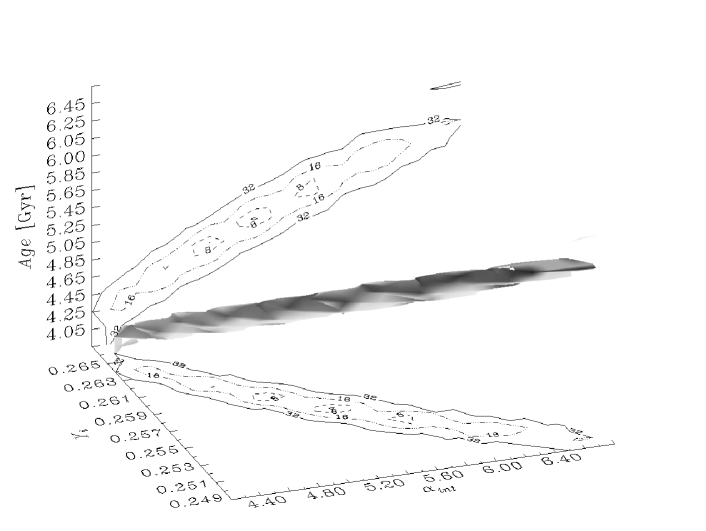
Fig. 1.: Fitting four observational quantities: $\chi^{2}=32$ surface and projections onto the $t-\alpha_{\rm int}$ and $Y_{i}-\alpha_{\rm int}$ planes in the parameter space

The models for this set of calculations include, with the exception of metal diffusion, all the physics of the best models of Schlattl et al. (1997), i.e. the special treatment of the convective gradient (Eq.(1)) and the inclusion of model atmospheres. They also start with the pre-main sequence evolution. Otherwise they agree with those of set B.

Contrary to the calculations of the previous section, for the present problem we have to scan the 3-dimensional parameter space. We did this with the following steps: $\triangle Y_{i}=0.001$, $\triangle\alpha_{\rm int}=0.1$, $\triangle t=2\cdot 10^{8}$ yrs. For $\alpha_{\rm int}=5.5$, we also used a finer $t$-grid of $5\cdot 10^{7}$ yrs (see below). As discussed in the previous section we now kept $Z_{i}$ constant at the value needed for $(Z/X)_{i}=(Z/X)_{\odot}$ in order to save computing time. In the investigation by Richard et al. (1997) the influence of varying $Z$ on $Y_{i}$ and the resulting solar model can be seen to be very small. We therefore do not expect that our results would change if we had not made this simplification.

Table 3.: Models for selected values of $\alpha_{\rm int}$ with the lowest $\chi^{2}$ of the problem fitting four observational quantities. $\alpha_{\rm int}$ is the interior value of the variable mixing-length parameter (see eq.1). For more details of the models, see the text. Ages are in $10^{9}$ yrs.

Case	$\alpha_{\rm int}$	$Y_{i}$	$t$	$L/L_{\odot}$	$T_{\rm eff}$ [K]	$R_{\rm cz}/R_{\odot}$	$Y_{s}$	$\chi^{2}$
C.1	4.5	0.263	4.45	1.0051	5780.0	0.7211	0.2359	14.84
C.2	4.7	0.261	4.65	1.0030	5777.0	0.7186	0.2336	7.36
C.3	5.0	0.259	4.85	1.0010	5778.0	0.7157	0.2316	3.91
C.4	5.1	0.259	4.85	1.0014	5782.4	0.7152	0.2317	8.27
C.5	5.3	0.257	5.05	0.9988	5777.1	0.7138	0.2294	3.46
C.6	5.5	0.255	5.25	0.9959	5771.3	0.7113	0.2271	11.58
C.6’	5.5	0.256	5.15	0.9977	5771.2	0.7119	0.2284	4.51
C.7	5.7	0.255	5.25	0.9965	5778.7	0.7108	0.2273	6.41
C.8	5.9	0.254	5.45	1.0035	5781.9	0.7097	0.2258	12.18
C.9	6.1	0.252	5.65	1.0001	5774.5	0.7070	0.2235	10.73

Figure1 shows $\chi^{2}$-surfaces and projected contour lines for our models. Apparently, there is no clearly defined sharp minimum which would allow a unique determination of the solar age from fitting the four quantities. Rather, there exists a long-stretched region of equally well fitting sets of parameters (including age). The separated minima visible in the projected contour plots are an artifact resulting from the grid in parameter space and the plot interpolation. In reality, the $\chi^{2}=8$ contour lines are connected. We have verified this by using a higher resolution in age for the case of $\alpha_{\rm int}=5.5$ (cf. Figs.2 and 4). Our grid of models in the $\alpha_{\rm int}$ and $Y_{i}$ parameter space is rather coarse due to the otherwise inhibitive number of solar evolution calculations. In Tab.3 we list those models with the lowest $\chi^{2}$ for several values of $\alpha_{\rm int}$. None of them is fitting all quantities very well (in particular, $Y_{\odot}$), as is indicated by the $\chi^{2}$-values which should be close to 1 for a good model. This is a confirmation of the fact that at the presently given accuracy of observations the theoretical models still contain significant deficits. Model C.5 is the best model of the real sun. Its age is within 10% of the presumed solar age. C.3 is within 6% of the true solar age at a slightly higher $\chi^{2}$. Given the uncertainty of $\approx$ 4% in the age determinations due to the time resolution we use, the true minimum could well be within 2-3 % of the solar age. The effect of a finer resolution in $\triangle t$ is demonstrated by model C.6’. Relative to C.6 the minimum is now located more accurately ($\chi^{2}=4.52$). The age of the true minimum is between 5.1 and 5.2 Gyr. It is evident that all models in Tab.3 have a surface helium content too low and consequently a rather low initial one, too.

3.3 Age determination by best-fit models to all observational data

Up to now we have used only two quantities derived from helioseismology. We are now going to include results about p-mode frequencies and sound speed. A simple inclusion of many frequencies or of the sound speed at many radial points as additional degrees of freedom would dominate the standard $\chi^{2}$-formula completely. In addition, since neither the frequencies nor the sound speed are statistically independent from $R_{\rm cz}$ or $Y_{\odot}$, the strict interpretation of $\chi^{2}$ is no longer valid. We therefore modify Eq.(2) to include two additional terms and interprete the resulting quantity as a function of merit, defined as

$$\tilde{\chi}^{2}=\sum_{i=1}^{6}{W_{i}},$$ (3)

where the first four terms are defined as in Eq.(2). The first additional term

$$W_{5}\equiv W_{\rm u}={\int_{0}^{1}(u_{\rm o}(x)-u_{\rm th}(x))^{2}dx\over\int_{0}^{1}\sigma_{u}^{2}(x)dx}$$ (4)

describes the deviation of the model sound speed $u_{\rm th}$ as a function of fractional radius $x=r/R_{\odot}$ from the helioseismologically inferred one ($u_{\rm o}$) weighted by the observational error $\sigma_{u}$. The other term

$$W_{6}\equiv W_{\nu}={\sum_{n=12}^{26}(\nu_{\rm o}(0,n)-\nu_{\rm th}(0,n))^{2}\over\sum_{j}\sigma_{\nu}^{2}(0,n)}$$ (5)

similarly is used to calculate the model goodness of the 15 frequencies $\nu(0,n)$ for a representative mode. We have selected the $l=0$ mode because it traces the whole solar interior. The choice of the 15 radial modes was dictated by the availability in the original papers.

Since the observational errors on $u$ and $\nu$ are extremely small, even the mean deviations $W_{\rm u}$ and $W_{\nu}$ still would dominate the function of merit. To allow the global quantities to retain their influence, we normalize the individual terms in Eq.(3) by their respective minimum values.

Fig. 2.: Quality of model fits using all solar quantities, illustrated by contour lines of the logarithm of the function-of-merit $\tilde{\chi}^{2}$, where all contributing terms have been normalized by their individual minimum value. The four panels are (from upper left to lower right) for $\alpha_{\rm int}=5.1,\,5.3,\,5.5,\,5.7$. Only parts of the parameter space has been investigated

Fig. 3.: As Fig.2, but for the case of fixed $Y_{i}=0.257$. The minimum at the center corresponds to model C.5

Fig. 4.: Contour-lines of $\log W_{\rm u}$ illustrating the quality of the models with respect to sound speed (fixed $\alpha_{\rm int}=5.5$; fine $t$-resolution). Note that $W_{\rm u}$ has not been normalized to its global minimum here

For evaluating $\tilde{\chi}^{2}$ the same solar evolution calculations as in the last section were used. The result of this age determination does not differ significantly from that of case C. In Fig.2 we show contour lines of $\log\tilde{\chi}^{2}$, the function-of-merit as defined by Eqs.(3-5), where the individual terms have been normalized by their respective minimum value. Evidently, there are only very small regions, where $\tilde{\chi}^{2}<10$, for all four cases of $\alpha_{\rm int}$ shown. For $\alpha_{\rm int}$ smaller than 4.7 and larger than 6.1 they vanish completely. The 3-dimensional isocontour resembles that of Fig.1 very much, therefore. The effect of a finer resolution in age ($\triangle t=5\cdot 10^{7}$ yrs) is seen in the lower left panel ($\alpha_{\rm int}=5.5$). Here, the contours for $\log\chi^{2}<3$ are still elongated, while in all other panels they form isolated wells. We have compared the shown $\alpha_{\rm int}=5.5$ contour lines with those for the same $t$-resolution as used for the other three panels ($\triangle t=2\cdot 10^{8}$ yrs) and found the same round shape of the $\log\chi^{2}<3$ contours. The minimum for this case deviates slightly from that of model C.6’, which was calculated with the same resolution. It is now at 5.2 Gyr but the same $Y_{i}=0.256$. The global minimum is reached (see Fig.2 upper right panel) for $\alpha_{\rm int}=5.3$ at $Y_{i}=0.257$ and age $t_{\odot}=5.05\cdot 10^{9}$ as for model C.5. For comparison, a cut at $Y_{i}=0.257$ is shown in Fig.3. The $\tilde{\chi}^{2}$ minimum again corresponds to model C.5.

The contribution of $W_{\rm u}$ and $W_{\nu}$ to $\tilde{\chi}^{2}$ is illustrated in Figs.4 and 5. Fig.4 demonstrates that the sound speed $\tilde{\chi}^{2}$-contours $W_{\rm u}$ outline a long-stretched valley enclosing the parameters of the best models without defining a clear minimum. Rather, the function-of-merit appears to be almost degenerate. Furthermore, the region of smallest $\chi^{2}$ is shifted towards higher ages and helium content with respect to the location of the best model. The shown case ($\alpha_{\rm int}=5.5$) is a typical one. $u$ cannot be used for age determinations.

Similarly, Fig.5 shows how the models fit the $l=0$ p-mode frequencies. The minima, though not very low, are very sharply defined, and the models providing the best fits for the complete problem also have a comparably low $W_{\nu}$. Model C.6, e.g., lies within the very narrow $\log W_{\nu}=2$ contour of the upper panel, which was plotted using the high $t$-resolution. The minimum within this countour is close to the position of model C.6, but at a slightly larger age. The position of model C.6’, which does not include the fit to the p-mode frequencies, but was calculated with the same high $t$-resolution, is outside the $\log W_{\nu}=2$ contour. Therefore, at a resolution of $5\cdot 10^{7}$ years, the minima of models C do no longer coincide with those of the p-mode fits. The complete fit (see Fig.2) incidentally is at the position of model C.6. Since in the complete fit we applied an – arbitrary – weighing of the contributing terms to $\tilde{\chi}^{2}$ by the normalization, the difference between these various minima gives a measure for a systematic age determination uncertainty of the order of 2%.

In the lower panel, Model C.6 can clearly be identified as the central minimum. The p-modes therefore add very important information in selecting the best-fit models and determining the solar age. The $W_{\nu}$-term also dominates $\tilde{\chi}^{2}$ and the contours of Fig.2. We cannot exclude that for an even higher resolution in $\alpha_{\rm int}$ or $Y_{i}$ the $W_{\nu}$ mimima deviate from those of the $\tilde{\chi}^{2}$ or of $\chi^{2}$ of models C, similar as in the demonstrated case of a higher $t$-resolution.

Fig. 5.: Contour-lines of the unnormalized $\log W_{\nu}$ illustrating the quality of the models with respect to the frequencies of the $l=0$-mode. Upper panel: for fixed parameter $\alpha_{\rm int}=5.5$ (fine $t$-resolution); lower panel: fixed $Y_{i}=0.255$

4 Discussion

If the solar age were to be determined from stellar models fitting observed solar quantities, we have shown that a priori an uncertainty of a factor of two would exist. The reason for this is the fact that apart from the global solar values – radius, effective temperature and $(Z/X)_{\odot}$ – the third quantity necessary to restrict mixing length parameter, initial helium content and age, has to be one derived from helioseismology. In our calculations, this was either the depth of the solar convective zone or the present photospheric helium abundance. Both quantities depend crucially on the effect of particle diffusion, though $R_{\rm cz}$ does less so (Tab.2). If this is not recognized, and diffusion not taken into account into the calculations, derived ages are by far too high (model sequences A & B without diffusion). If diffusion is taken into account, the predicted ages can be as accurate as 10%, if $R_{\rm cz}$ is the third parameter, but are too low by up to 40% for the allowed range of $Y_{\odot}$. The latter fact indicates that either diffusion is too effective in the models or that $Y_{\odot}$ is rather at the lower boundary of the present determinations.

Including both of these helioseismological quantities in fitting the present sun, ${\chi}^{2}$-fits using “best-physics-models” yield ages that agree to 10% or better with the solar age. However, none of the models is a good model for the Sun with ${\chi}^{2}\approx 1$ and there is no clear global ${\chi}^{2}$-minimum fit. If we generously accept all models of Tab.3 with ${\chi}^{2}\mathrel{\mathchoice{\vbox{\offinterlineskip\halign{\hfil$\displaystyle#$\hfil\cr<\cr\sim\cr}}}{\vbox{\offinterlineskip\halign{\hfil$\textstyle#$\hfil\cr<\cr\sim\cr}}}{\vbox{\offinterlineskip\halign{\hfil$\scriptstyle#$\hfil\cr<\cr\sim\cr}}}{\vbox{\offinterlineskip\halign{\hfil$\scriptscriptstyle#$\hfil\cr<\cr\sim\cr}}}}10$ (approx. $3\sigma$), the solar age could range between 4.65 and 5.65 Gyr, being slightly too high. Therefore, a systematic error in the models is still present.

Adding sound speed and p-mode frequencies to the fits, the best-fitting models remain nearly the same as in the previous case, if we normalize the individual contributions to the function of merit. This is necessary, since all solar models do not predict p-mode frequencies and sound speed throughout the Sun with sufficient accuracy for the extremely low errors in the observations. Since the various quantities used in this fit are no longer independent of each other, the function of merit, though still denoted by $\tilde{\chi}^{2}$, no longer has any statistical meaning. While sound speed does not provide helpful information for age determinations, the p-mode frequencies are extremely sensitive to deviations of the models from the observed Sun. In fact, though all models are poor fits for the p-modes, the function-of-merit minima are extremely sharp and coincide with the parameters also yielding the best fits for the previous case of 4 solar parameters, as long as we use age-steps of $2\cdot 10^{8}$ yrs. At a four times higher resolution, the various $\tilde{\chi}^{2}$-minima do no longer coincide, but the location of the “true” minimum remains subject to the exact definition of $\tilde{\chi}^{2}$. p-mode frequencies alone might suffice for finding best-fit parameters, including the solar age.

Table 4.: $\chi^{2}$-minima of the problem fitting four observational quantities for $\alpha_{\rm int}=5.3$ and two values of $Y-i$. In these calculations metal diffusion has been taken into account and the high resolution in time has been applied. For comparison, model C.5 is repeated

Case	$\alpha_{\rm int}$	$Y_{i}$	$t$	$L/L_{\odot}$	$T_{\rm eff}$ [K]	$R_{\rm cz}/R_{\odot}$	$Y_{s}$	$\chi^{2}$
D.1	5.3	0.257	5.00	0.9970	5779.8	0.7182	0.2295	8.40
D.2	5.3	0.256	5.15	0.9994	5774.5	0.7180	0.2277	9.42
C.5	5.3	0.257	5.05	0.9988	5777.1	0.7138	0.2294	3.46

We have for one special case investigated the effect of metal diffusion ($\alpha_{\rm int}=5.3$; $\triangle t=5\cdot 10^{7}$; cf. model C.5). Table4 lists the minima for two different choices of $Y_{i}$. Compared to C.5, model D.1 (same $Y_{i}$) has a minimum of higher $\chi^{2}$ at a slightly lower age. A better fit is found for a lower $Y_{i}$ but at a higher age (D.2). At least for this value of $\alpha_{\rm int}$, we conclude that the consideration of metal diffusion would lead to a $\chi^{2}$-minimum at a much higher age. Whether the global $\chi^{2}$-minimum would also be shifted towards an higher age, can only be decided after the (time-consuming) calculations for all parameters have been done. From the fact that the depth of the convective zone has increased for models D, we infer that only the C-models with a low value for $R_{\rm cz}/R_{\odot}$ could give the global $\chi^{2}$-minimum, if metal diffusion were included. Those, however, already have ages too high. It might be that the inclusion of “better” physics in this case leads to a larger error in the age determination.

The implications for stellar age determinations are not straightforward. Evidently, the physical input used today for the standard solar model (including diffusion) provides the most accurate age determination. It therefore should be used in stellar models in general. If direct measurements of stellar parameters (mass, luminosity, effective temperature) are available, the derived ages can be expected to be comparably accurate as in the solar case provided the observations are as accurate as for the Sun.

The inclusion of diffusion is the most important aspect of solar age determinations performed as in the present paper. If it is neglected, the derived ages are unacceptable. This is due to our knowledge about the helium content or depth of the solar convective zone. For other stars, this information will not be available directly. Evolutionary ages will then depend solely on the assumed initial helium content, no matter whether diffusion is taken into account or not. Paczyński (1996a) argues that detached eclipsing binaries will provide the possibility to determine age and (initial) helium content at the same time. In this case, diffusion most likely has to be included, since the central helium content is changed by diffusion and this influences the main-sequence lifetime. Otherwise, an additional uncertainty of about 5% (Chaboyer 1995) is added. Note that for old systems, the relative error due to a wrong helium content is smaller than in the solar case, because it leads to a luminosity change roughly constant for the whole main sequence evolution. Absolute errors could be of up to a few Gyr.

For age determination methods based on differential quantities like the brightness difference between turn-off and horizontal branch the situation is more complicated. If the defects of the stellar evolution calculations, which lead to the solar age errors, affect the different stellar evolution stages systematically, the ages based on differential methods could be more accurate than the results found here indicate. (There are, however, many other, probably more severe sources of errors, like the conversion from theoretical to observational brightness.) This, however, has to be investigated in detail (Castellani et al. 1997).

To summarize, we have demonstrated that even with the best observational data available, present stellar evolution calculations cannot be expected to yield ages with errors less than 10%. Hydrogen/helium diffusion is an absolutely necessary ingredient to reach this level of accuracy. We have not investigated, whether the inclusion of metal-diffusion would lead to a more accurate solar age, because in most stellar evolution calculations this most likely will not be included due to computational limitations.

• It is a pleasure to thank B.Paczyński for initiating the present work by asking us a simple, but fundamental question and for his continuing support and stimulating discussions. H.S. was supported by the “Sonderforschungsbereich 375-95 für Astro-Teilchenphysik” of the Deutsche Forschungsgemeinschaft.

References

- 1 Alexander D.R., Fergusson J.W., 1994, ApJ 437, 879
- 2 Basu S., Christensen-Dalsgaard J., Schou J., Thompson M.J., Tomczyk S., 1996, ApJ 460, 1064
- 3 Castellani V. etal., 1994, Phys.Rev.C 50, 4749
- 4 Castellani V., Ciacio F., Degl’Innocenti S., Fiorentini G., 1997, preprint astro-ph9705035
- 5 Chaboyer B., 1995, ApJL 444, 9
- 6 Chaboyer B., Kim Y.-C., 1995, ApJ 454, 767
- 7 Christensen-Dalsgaard J., Gough D.O., Thompson M.J., 1991, ApJ 378, 413
- 8 D’Antona F., Caloi V., Mazzitelli I., 1997, ApJ 477, 519
- 9 Degl’Innocenti S., Dziembowski W.A., Fiorentini G., Ricci B., 1997, preprint astro-ph9612053
- 10 Dziembowski W.A., Goode P.R., Pamyatnych A.A., Sienkiewiecz R., 1994, ApJ 432, 417
- 11 Elsworth Y. etal., 1994, ApJ 434, 801
- 12 Grevesse N., Noels A., 1993, Phys.Scripta T47, 133
- 13 Iglesias C.A., Rogers F.J., 1996, ApJ 464, 943
- 14 Kaluzny J., Kubiak M., Szymanński M., Udalski A., Krzeminśki W., Mateo M., 1996, A&AS 120, 139
- 15 Libbrecht K.G., Woodard M.F., Kaufman J.M., 1990, ApJS 74, 1129
- 16 Mazzitelli I., D’Antona F., Caloi V., 1995, A&A 302, 382
- 17 Paczyński B., 1996, in xxx (ed.), Variable stars and the astrophysical returns of microlensing surveys, IAP, July 7-12, 1996, in press
- 18 Paczyński B., 1996, in Turok N. (ed.), Critical Dialogues in Cosmology, Proceedings of the Princeton University, Conference June 24-27, 1996, Princeton, University Press, in press
- 19 Richard O., Vauclair S., Charbonnel C., Dziembowski W.A., 1997, A&A, submitted
- 20 Rogers F.J., Iglesias C.A., 1992, ApJS 79, 507
- 21 Rogers F.J., Swenson F.J., Iglesias C.A., 1996, ApJ 456, 902
- 22 Salaris M., Degl’Innocenti S., Weiss A., 1997, ApJ 479, 665
- 23 Schlattl H., Weiss A., Ludwig H.-G., 1997, A&A, in press
- 24 Schröder P., Pols O.R., Eggleton P., 1997, MNRAS 285, 696
- 25 Shi X., 1995, ApJ 446, 637
- 26 Stetson P.B., VandenBerg D.A., Bolte M., 1996, PASP 108, 560
- 27 Thoul A.A., Bahcall J.N., Loeb A., 1994, ApJ 421, 828
- 28 Weiss A., Schlattl, H., 1997, in preparation
- 29 Weiss A., Keady J.J., Magee N.H., 1990, Atomic Data and Nuclear Data Tables 45, 209