A CMB Polarization Primer

Abstract

We present a pedagogical and phenomenological introduction to the study of cosmic microwave background (CMB) polarization to build intuition about the prospects and challenges facing its detection. Thomson scattering of temperature anisotropies on the last scattering surface generates a linear polarization pattern on the sky that can be simply read off from their quadrupole moments. These in turn correspond directly to the fundamental scalar (compressional), vector (vortical), and tensor (gravitational wave) modes of cosmological perturbations. We explain the origin and phenomenology of the geometric distinction between these patterns in terms of the so-called electric and magnetic parity modes, as well as their correlation with the temperature pattern. By its isolation of the last scattering surface and the various perturbation modes, the polarization provides unique information for the phenomenological reconstruction of the cosmological model. Finally we comment on the comparison of theory with experimental data and prospects for the future detection of CMB polarization.

1 Introduction

Why should we be concerned with the polarization of the cosmic microwave background (CMB) anisotropies? That the CMB anisotropies are polarized is a fundamental prediction of the gravitational instability paradigm. Under this paradigm, small fluctuations in the early universe grow into the large scale structure we see today. If the temperature anisotropies we observe are indeed the result of primordial fluctuations, their presence at last scattering would polarize the CMB anisotropies themselves. The verification of the (partial) polarization of the CMB on small scales would thus represent a fundamental check on our basic assumptions about the behavior of fluctuations in the universe, in much the same way that the redshift dependence of the CMB temperature is a test of our assumptions about the background cosmology.

Furthermore, observations of polarization provide an important tool for reconstructing the model of the fluctuations from the observed power spectrum (as distinct from fitting an a priori model prediction to the observations). The polarization probes the epoch of last scattering directly as opposed to the temperature fluctuations which may evolve between last scattering and the present. This localization in time is a very powerful constraint for reconstructing the sources of anisotropy. Moreover, different sources of temperature anisotropies (scalar, vector and tensor) give different patterns in the polarization: both in its intrinsic structure and in its correlation with the temperature fluctuations themselves. Thus by including polarization information, one can distinguish the ingredients which go to make up the temperature power spectrum and so the cosmological model.

Finally, the polarization power spectrum provides information complementary to the temperature power spectrum even for ordinary (scalar or density) perturbations. This can be of use in breaking parameter degeneracies and thus constraining cosmological parameters more accurately. The prime example of this is the degeneracy, within the limitations of cosmic variance, between a change in the normalization and an epoch of “late” reionization.

Yet how polarized are the fluctuations? The degree of linear polarization is directly related to the quadrupole anisotropy in the photons when they last scatter. While the exact properties of the polarization depend on the mechanism for producing the anisotropy, several general properties arise. The polarization peaks at angular scales smaller than the horizon at last scattering due to causality. Furthermore, the polarized fraction of the temperature anisotropy is small since only those photons that last scattered in an optically thin region could have possessed a quadrupole anisotropy. The fraction depends on the duration of last scattering. For the standard thermal history, it is $10\%$ on a characteristic scale of tens of arcminutes. Since temperature anisotropies are at the $10^{-5}$ level, the polarized signal is at (or below) the $10^{-6}$ level, or several $\mu$K, representing a significant experimental challenge.

Our goal here is to provide physical intuition for these issues. For mathematical details, we refer the reader to [Kamionkowski et al.] (1997), [Zaldarriaga & Seljak] (1997), [Hu & White] (1997) as well as pioneering work by [Bond & Efstathiou] (1984) and [Polnarev] (1985). The outline of the paper is as follows. We begin in §2 by examining the general properties of polarization formation from Thomson scattering of scalar, vector and tensor anisotropy sources. We discuss the properties of the resultant polarization patterns on the sky and their correlation with temperature patterns in §3. These considerations are applied to the reconstruction problem in §4. The current state of observations and techniques for data analysis are reviewed in §5. We conclude in §6 with comments on future prospects for the measurement of CMB polarization.

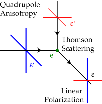
Figure 1: Thomson scattering of radiation with a quadrupole anisotropy generates linear polarization. Blue colors (thick lines) represent hot and red colors (thin lines) cold radiation.

2 Thomson Scattering

2.1 From Anisotropies to Polarization

The Thomson scattering cross section depends on polarization as (see e.g. [Chandrasekhar] 1960)

$${d\sigma_{T}\over d\Omega}\propto|\hat{\epsilon}\cdot\hat{\epsilon}^{\prime}|^{2}\,,$$ (1)

where $\hat{\epsilon}$ ($\hat{\epsilon}^{\prime}$) are the incident (scattered) polarization directions. Heuristically, the incident light sets up oscillations of the target electron in the direction of the electric field vector ${\bf E}$, i.e. the polarization. The scattered radiation intensity thus peaks in the direction normal to, with polarization parallel to, the incident polarization. More formally, the polarization dependence of the cross section is dictated by electromagnetic gauge invariance and thus follows from very basic principles of fundamental physics.

If the incoming radiation field were isotropic, orthogonal polarization states from incident directions separated by $90^{\circ}$ would balance so that the outgoing radiation would remain unpolarized. Conversely, if the incident radiation field possesses a quadrupolar variation in intensity or temperature (which possess intensity peaks at $90^{\circ}=\pi/2$ separations), the result is a linear polarization of the scattered radiation (see Fig. 1). A reversal in sign of the temperature fluctuation corresponds to a $90^{\circ}$ rotation of the polarization, which reflects the spin-2 nature of polarization.

In terms of a multipole decomposition of the radiation field into spherical harmonics, $Y_{\ell}^{m}(\theta,\phi)$, the five quadrupole moments are represented by $\ell=2$, $m=0,\pm 1,\pm 2$. The orthogonality of the spherical harmonics guarantees that no other moment can generate polarization from Thomson scattering. In these spherical coordinates, with the north pole at $\theta=0$, we call a N-S (E-W) polarization component $Q>0$ ($Q<0$) and a NE-SW (NW-SE) component $U>0$ ($U<0$). The polarization amplitude and angle clockwise from north are

$$P=\sqrt{Q^{2}+U^{2}},\qquad\alpha={1\over 2}\tan^{-1}(U/Q)\,.$$ (2)

Alternatively, the Stokes parameters $Q$ and $U$ represent the diagonal and off diagonal components of the symmetric, traceless, $2\times 2$ intensity matrix in the polarization plane spanned by ($\hat{\bf e}_{\theta}$, $\hat{\bf e}_{\phi}$),

$$E_{i}^{*}E_{j}-{1\over 2}\delta_{ij}E^{2}\propto Q\sigma_{3}+U\sigma_{1}\,,$$ (3)

where $\sigma_{i}$ are the Pauli matrices and circular polarization is assumed absent.

If Thomson scattering is rapid, then the randomization of photon directions that results destroys any quadrupole anisotropy and polarization. The problem of understanding the polarization pattern of the CMB thus reduces to understanding the quadrupolar temperature fluctuations at last scattering.

Temperature perturbations have 3 geometrically distinct sources: the scalar (compressional), vector (vortical) and tensor (gravitational wave) perturbations. Formally, they form the irreducible basis of the symmetric metric tensor. We shall consider each of these below and show that the scalar, vector, and tensor quadrupole anisotropy correspond to $m=0,\pm 1,\pm 2$ respectively. This leads to different patterns of polarization for the three sources as we shall discuss in §3.

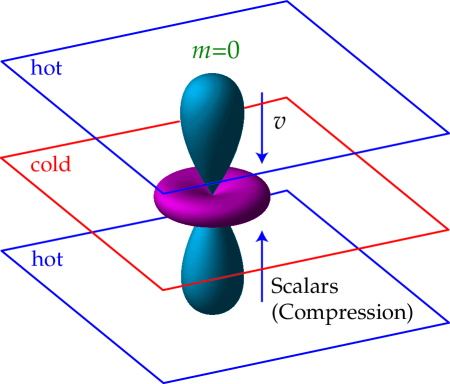
Figure 2: The scalar quadrupole moment ($\ell=2,m=0$). Flows from hot (blue) regions into cold (red), ${\bf v}\parallel{\bf k}$, produce the azimuthally symmetric pattern $Y_{2}^{0}$ depicted here.

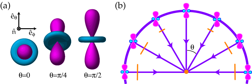
Figure 3: The transformation of quadrupole anisotropies into linear polarization. (a) The orientation of the quadrupole moment with respect to the scattering direction $\hat{\bf n}$ determines the sense and magnitude of the polarization. It is aligned with the cold (red, long) lobe in the $\hat{\bf e}_{\theta}\otimes\hat{\bf e}_{\phi}$ tangent plane. (b) In spherical coordinates where $\hat{\bf n}\cdot\hat{\bf k}=\cos\theta$, the polarization points north-south ($Q$) with magnitude varying as $\sin^{2}\theta$ for scalar fluctuations.

2.2 Scalar Perturbations

The most commonly considered and familiar types of perturbations are scalar modes. These modes represent perturbations in the (energy) density of the cosmological fluid(s) at last scattering and are the only fluctuations which can form structure though gravitational instability.

Consider a single large-scale Fourier component of the fluctuation, i.e. for the photons, a single plane wave in the temperature perturbation. Over time, the temperature and gravitational potential gradients cause a bulk flow, or dipole anisotropy, of the photons. Both effects can be described by introducing an “effective” temperature

$$(\Delta T/T)_{\rm eff}=\Delta T/T+\Psi\,,$$ (4)

where $\Psi$ is the gravitational potential. Gradients in the effective temperature always create flows from hot to cold effective temperature. Formally, both pressure and gravity act as sources of the momentum density of the fluid in a combination that is exactly the effective temperature for a relativistic fluid.

To avoid confusion, let us explicitly consider the case of adiabatic fluctuations, where initial perturbations to the density imply potential fluctuations that dominate at large scales. Here gravity overwhelms pressure in overdense regions causing matter to flow towards density peaks initially. Nonetheless, overdense regions are effectively cold initially because photons must climb out of the potential wells they create and hence lose energy in the process. Though flows are established from cold to hot temperature regions on large scales, they still go from hot to cold effective temperature regions. This property is true more generally of our adiabatic assumption: we hereafter refer only to effective temperatures to keep the argument general.

Let us consider the quadrupole component of the temperature pattern seen by an observer located in a trough of a plane wave. The azimuthal symmetry in the problem requires that ${\bf v}\parallel{\bf k}$ and hence the flow is irrotational ${\bf\nabla}\times{\bf v}=0$. Because hotter photons from the crests flow into the trough from the $\pm\hat{\bf k}$ directions while cold photons surround the observer in the plane, the quadrupole pattern seen in a trough has an $m=0$,

$$Y_{2}^{0}\propto 3\cos^{2}\theta-1\,,$$ (5)

structure with angle $\hat{\bf n}\cdot\hat{\bf k}=\cos\theta$ (see Fig. 2). The opposite effect occurs at the crests, reversing the sign of the quadrupole but preserving the $m=0$ nature in its local angular dependence. The full effect is thus described by a local quadrupole modulated by a plane wave in space, $-Y_{2}^{0}(\hat{\bf n})\exp(i{\bf k}\cdot{\bf x})$, where the sign denotes the fact that photons flowing into cold regions are hot. This infall picture must be modified slightly on scales smaller than the sound horizon where pressure plays a role (see §3.3.2), however the essential property that the flows are parallel to $\hat{\bf k}$ and thus generate an $m=0$ quadrupole remains true.

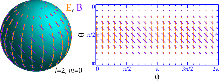
Figure 4: Polarization pattern for $\ell=2$, $m=0$, note the azimuthal symmetry. The scattering of a scalar $m=0$ quadrupole perturbation generates the electric $E$ (yellow, thick lines) pattern on the sphere. Its rotation by $45^{\circ}$ represents the orthogonal magnetic $B$ (purple, thin lines) pattern. Animation (available at http://www.sns.ias.edu/$\sim$whu/polar/scalaran.html): as the line of sight $\hat{\bf n}$ changes, the lobes of the quadrupole rotate in and out of the tangent plane. The polarization follows the orientation of the colder (red) lobe in the tangent plane.

The sense of the quadrupole moment determines the polarization pattern through Thomson scattering. Recall that polarized scattering peaks when the temperature varies in the direction orthogonal to $\hat{\bf n}$. Consider then the tangent plane $\hat{\bf e}_{\theta}\otimes\hat{\bf e}_{\phi}$ with normal $\hat{\bf n}$. This may be visualized in an angular “lobe” diagram such as Fig. 2 as a plane which passes through the “origin” of the quadrupole pattern perpendicular to the line of sight. The polarization is maximal when the hot and cold lobes of the quadrupole are in this tangent plane, and is aligned with the component of the colder lobe which lies in the plane. As $\theta$ varies from $0$ to $\pi/2$ (pole to equator) the temperature differences in this plane increase from zero (see Fig. 3a). The local polarization at the crest of the temperature perturbation is thus purely in the N-S direction tapering off in amplitude toward the poles (see Fig. 3b). This pattern represents a pure $Q$-field on the sky whose amplitude varies in angle as an $\ell=2$, $m=0$ tensor or spin-2 spherical harmonic

$$Q=\sin^{2}\theta,\qquad U=0.$$ (6)

In different regions of space, the plane wave modulation of the quadrupole can change the sign of the polarization, but not its sense.

This pattern (Fig. 4, yellow lines) is of course not the only logical possibility for an $\ell=2$, $m=0$ polarization pattern. Its rotation by $45^{\circ}$ is also a valid configuration (purple lines). This represents a pure NW-SE (and by sign reversal NE-SW), or $U$-polarization pattern. We return in §3.3 to consider the geometrical distinction between the two patterns, the electric and magnetic modes.

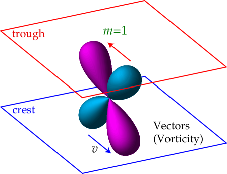
Figure 5: The vector quadrupole moment ($\ell=2$, $m=1$). Since ${\bf v}\perp{\bf k}$, the Doppler effect generates a quadrupole pattern with lobes $45^{\circ}$ from ${\bf v}$ and ${\bf k}$ that is spatially out of phase (interplane peaks) with ${\bf v}$.

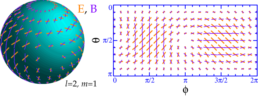
Figure 6: Polarization pattern for $\ell=2$, $m=1$. The scattering of a vector $(m=1)$ quadrupole perturbation generates the $E$ pattern (yellow, thick lines) as opposed to the $B$, (purple, thin lines) pattern. Animation (available at http://www.sns.ias.edu/$\sim$whu/polar/vectoran.html): same as for scalars.

2.3 Vector Perturbations

Vector perturbations represent vortical motions of the matter, where the velocity field ${\bf v}$ obeys ${\bf\nabla}\cdot{\bf v}=0$ and ${\bf\nabla}\times{\bf v}\neq 0$, similar to “eddies” in water. There is no associated density perturbation, and the vorticity is damped by the expansion of the universe as are all motions that are not enhanced by gravity. However, the associated temperature fluctuations, once generated, do not decay as both $\Delta T$ and $T$ scale similarly with the expansion. For a plane wave perturbation, the velocity field ${\bf v}\perp{\bf k}$ with direction reversing in crests and troughs (see Fig. 5). The radiation field at these extrema possesses a dipole pattern due to the Doppler shift from the bulk motion. Quadrupole variations vanish here but peak between velocity extrema. To see this, imagine sitting between crests and troughs. Looking up toward the trough, one sees the dipole pattern projected as a hot and cold spot across the zenith; looking down toward the crest, one sees the projected dipole reversed. The net effect is a quadrupole pattern in temperature with $m=\pm 1$

$$Y_{2}^{\pm 1}\propto\sin\theta\cos\theta e^{\pm i\phi}.$$ (7)

The lobes are oriented at 45^∘ from ${\bf k}$ and ${\bf v}$ since the line of sight velocity vanishes along ${\bf k}$ and at 90 degrees to ${\bf k}$ here. The latter follows since midway between the crests and troughs ${\bf v}$ itself is zero. The full quadrupole distribution is therefore described by $-iY_{2}^{\pm 1}(\hat{\bf n})\exp(i{\bf k}\cdot{\bf x})$, where $i$ represents the spatial phase shift of the quadrupole with respect to the velocity.

Thomson scattering transforms the quadrupole temperature anisotropy into a local polarization field as before. Again, the pattern may be visualized from the intersection of the tangent plane to $\hat{\bf n}$ with the lobe pattern of Fig. 5. At the equator ($\theta=\pi/2$), the lobes are oriented $45^{\circ}$ from the line of sight $\hat{\bf n}$ and rotate into and out of the tangent plane with $\phi$. The polarization pattern here is a pure $U$-field which varies in magnitude as $\sin\phi$. At the pole $\theta=0$, there are no temperature variations in the tangent plane so the polarization vanishes. Other angles can equally well be visualized by viewing the quadrupole pattern at different orientations given by $\hat{\bf n}$.

The full $\ell=2$, $m=1$ pattern,

$$Q=-\sin\theta\cos\theta e^{i\phi},\qquad U=-i\sin\theta e^{i\phi}$$ (8)

is displayed explicitly in Fig. 6 (yellow lines, real part). Note that the pattern is dominated by $U$-contributions especially near the equator. The similarities and differences with the scalar pattern will be discussed more fully in §3.

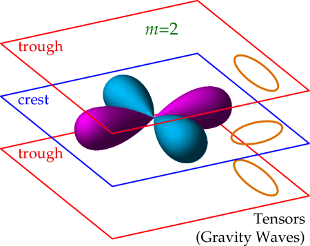
Figure 7: The tensor quadrupole moment $(m=2)$. Since gravity waves distort space in the plane of the perturbation, changing a circle of test particles into an ellipse, the radiation acquires an $m=2$ quadrupole moment.

2.4 Tensor Perturbations

Tensor fluctuations are transverse-traceless perturbations to the metric, which can be viewed as gravitational waves. A plane gravitational wave perturbation represents a quadrupolar “stretching” of space in the plane of the perturbation (see Fig. 7). As the wave passes or its amplitude changes, a circle of test particles in the plane is distorted into an ellipse whose semi-major axis $\rightarrow$ semi-minor axis as the spatial phase changes from crest $\rightarrow$ trough (see Fig. 7, yellow ellipses). Heuristically, the accompanying stretching of the wavelength of photons produces a quadrupolar temperature variation with an $m=\pm 2$ pattern

$$Y_{2}^{\pm 2}\propto\sin^{2}\theta e^{\pm 2i\phi}$$ (9)

in the coordinates defined by $\hat{\bf k}$.

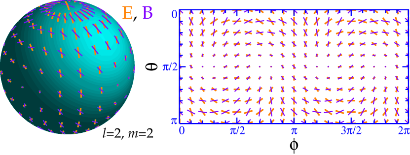
Figure 8: Polarization pattern for $\ell=2$ $m=2$. Scattering of a tensor $m=2$ perturbation generates the $E$ (yellow, thick lines) pattern as opposed to the $B$ (purple, thin lines) pattern. Animation (available at http://www.sns.ias.edu/$\sim$whu/polar/tensoran.html): same as for scalars and vectors.

Thomson scattering again produces a polarization pattern from the quadrupole anisotropy. At the equator, the quadrupole pattern intersects the tangent ($\hat{\bf e}_{\theta}\otimes\hat{\bf e}_{\phi}$) plane with hot and cold lobes rotating in and out of the $\hat{\bf e}_{\phi}$ direction with the azimuthal angle $\phi$. The polarization pattern is therefore purely $Q$ with a $\cos(2\phi)$ dependence. At the pole, the quadrupole lobes lie completely in the polarization plane and produces the maximal polarization unlike the scalar and vector cases. The full pattern,

$$Q=(1+\cos^{2}\theta)e^{2i\phi},\qquad U=-2i\cos\theta e^{2i\phi},$$ (10)

is shown in Fig. 8 (real part). Note that $Q$ and $U$ are present in nearly equal amounts for the tensors.

3 Polarization Patterns

The considerations of §2 imply that scalars, vectors, and tensors generate distinct patterns in the polarization of the CMB. However, although they separate cleanly into $m=0,\pm 1,\pm 2$ polarization patterns for a single plane wave perturbation in the coordinate system referenced to ${\bf k}$, in general there will exist a spectrum of fluctuations each with a different ${\bf k}$. Therefore the polarization pattern on the sky does not separate into $m=0,\pm 1,\pm 2$ modes. In fact, assuming statistical isotropy, one expects the ensemble averaged power for each multipole $\ell$ to be independent of $m$. Nonetheless, certain properties of the polarization patterns discussed in the last section do survive superposition of the perturbations: in particular, its parity and its correlation with the temperature fluctuations. We now discuss how one can describe polarization patterns on the sky arising from a spectrum of ${\bf k}$ modes.

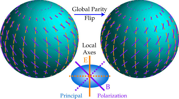
Figure 9: The electric ($E$) and magnetic ($B$) modes are distinguished by their behavior under a parity transformation $\hat{\bf n}\rightarrow-\hat{\bf n}$. $E$-modes have $(-1)^{\ell}$ and $B$-modes have $(-1)^{\ell+1}$ parity; here $(\ell=2,m=0)$, even and odd respectively. The local distinction between the two is that the polarization axis is aligned with the principle axes of the polarization amplitude for $E$ and crossed with them for $B$. Dotted lines represent a sign reversal in the polarization.

3.1 Electric and Magnetic Modes

Any polarization pattern on the sky can be separated into “electric” ($E$) and “magnetic” ($B$) components. This decomposition is useful both observationally and theoretically, as we will discuss below. There are two equivalent ways of viewing the modes that reflect their global and local properties respectively. The nomenclature reflects the global property. Like multipole radiation, the harmonics of an $E$-mode have $(-1)^{\ell}$ parity on the sphere, whereas those of a $B$-mode have $(-1)^{\ell+1}$ parity. Under $\hat{\bf n}\rightarrow-\hat{\bf n}$, the $E$-mode thus remains unchanged for even $\ell$, whereas the $B$-mode changes sign as illustrated for the simplest case $\ell=2,m=0$ in Fig. 9 (recall that a rotation by 90^∘ represents a change in sign). Note that the $E$ and $B$ multipole patterns are $45^{\circ}$ rotations of each other, i.e. $Q\rightarrow U$ and $U\rightarrow-Q$. Since this parity property is obviously rotationally invariant, it will survive integration over $\hat{\bf k}$.

The local view of $E$ and $B$-modes involves the second derivatives of the polarization amplitude (second derivatives because polarization is a tensor or spin-2 object). In much the same way that the distinction between electric and magnetic fields in electromagnetism involves vanishing of gradients or curls (i.e. first derivatives) for the polarization there are conditions on the second (covariant) derivatives of $Q$ and $U$. For an $E$-mode, the difference in second (covariant) derivatives of $U$ along $\hat{\bf e}_{\theta}$ and $\hat{\bf e}_{\phi}$ vanishes as does that for $Q$ along $\hat{\bf e}_{\theta}+\hat{\bf e}_{\phi}$ and $\hat{\bf e}_{\theta}-\hat{\bf e}_{\phi}$. For a $B$-mode, $Q$ and $U$ are interchanged. Recalling that a $Q$-field points in the $\hat{\bf e}_{\theta}$ or $\hat{\bf e}_{\phi}$ direction and a $U$-field in the crossed direction, we see that the Hessian or curvature matrix of the polarization amplitude has principle axes in the same sense as the polarization for $E$ and 45^∘ crossed with it for $B$ (see Fig. 9). Stated another way, near a maximum of the polarization (where the first derivative vanishes) the direction of greatest change in the polarization is parallel/perpendicular and at $45^{\circ}$ degrees to the polarization in the two cases.

The distinction is best illustrated with examples. Take the simplest case of $\ell=2$, $m=0$ where the $E$-mode is a $Q=\sin^{2}\theta$ field and the $B$-mode is a $U=\sin^{2}\theta$ field (see Fig. 4). In both cases, the major axis of the curvature lies in the $\hat{\bf e}_{\theta}$ direction. For the $E$-mode, this is in the same sense; for the $B$-mode it is crossed with the polarization direction. The same holds true for the $m=1,2$ modes as can be seen by inspection of Fig. 6 and 8.

3.2 Electric and Magnetic Spectra

Thomson scattering can only produce an $E$-mode locally since the spherical harmonics that describe the temperature anisotropy have $(-1)^{\ell}$ electric parity. In Figs. 4, 6, and 8, the $\ell=2$, $m=0,1,2$ $E$-mode patterns are shown in yellow. The $B$-mode represents these patterns rotated by $45^{\circ}$ and are shown in purple and cannot be generated by scattering. In this way, the scalars, vectors, and tensors are similar in that scattering produces a local $\ell=2$ $E$-mode only.

However, the pattern of polarization on the sky is not simply this local signature from scattering but is modulated over the last scattering surface by the plane wave spatial dependence of the perturbation (compare Figs. 3 and 10). The modulation changes the amplitude, sign, and angular structure of the polarization but not its nature, e.g. a $Q$-polarization remains $Q$. Nonetheless, this modulation generates a $B$-mode from the local $E$-mode pattern.

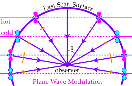
Figure 10: Modulation of the local pattern Fig. 3b by plane wave fluctuations on the last scattering surface. Yellow points represent polarization out of the plane with magnitude proportional to sign. The plane wave modulation changes the amplitude and sign of the polarization but does not mix $Q$ and $U$. Modulation can mix $E$ and $B$ however if $U$ is also present.

The reason why this occurs is best seen from the local distinction between $E$ and $B$-modes. Recall that $E$-modes have polarization amplitudes that change parallel or perpendicular to, and $B$-modes in directions $45^{\circ}$ away from, the polarization direction. On the other hand, plane wave modulation always changes the polarization amplitude in the direction $\hat{\bf k}$ or N-S on the sphere. Whether the resultant pattern possesses $E$ or $B$-contributions depends on whether the local polarization has $Q$ or $U$-contributions.

For scalars, the modulation is of a pure $Q$-field and thus its $E$-mode nature is preserved ([Kamionkowski et al.] 1997; [Zaldarriaga & Seljak] 1997). For the vectors, the $U$-mode dominates the pattern and the modulation is crossed with the polarization direction. Thus vectors generate mainly $B$-modes for short wavelength fluctuations ([Hu & White] 1997). For the tensors, the comparable $Q$ and $U$ components of the local pattern imply a more comparable distribution of $E$ and $B$ modes at short wavelengths (see Fig. 11a).

These qualitative considerations can be quantified by noting that plane wave modulation simply represent the addition of angular momentum from the plane wave ($Y_{\ell}^{0}$) with the local spin angular dependence. The result is that plane wave modulation takes the $\ell=2$ local angular dependence to higher $\ell$ (smaller angles) and splits the signal into $E$ and $B$ components with ratios which are related to Clebsch-Gordan coefficients. At short wavelengths, these ratios are $B/E=0,6,8/13$ in power for scalars, vectors, and tensors (see Fig. 11b and [Hu & White] 1997).

The distribution of power in multipole $\ell$-space is also important. Due to projection, a single plane wave contributes to a range of angular scales $\ell\mathrel{\hbox to0.0pt{\lower 3.0pt\hbox{$\mathchar 536\relax$}\hss}\raise 2.0pt\hbox{$\mathchar 316\relax$}}kr$ where $r$ is the comoving distance to the last scattering surface. From Fig. 10, we see that the smallest angular, largest $\ell\approx kr$ variations occur on lines of sight $\hat{\bf n}\cdot\hat{\bf k}=0$ or $\theta=\pi/2$ though a small amount of power projects to $\ell\ll kr$ as $\theta\rightarrow 0$. The distribution of power in multipole space of Fig. 11b can be read directly off the local polarization pattern. In particular, the region near $\theta=\pi/2$ shown in Fig. 11a determines the behavior of the main contribution to the polarization power spectrum.

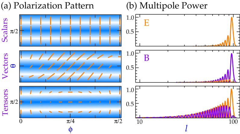
Figure 11: The $E$ and $B$ components of a plane wave perturbation. (a) Modulation of the local $E$-quadrupole pattern (yellow) from scattering by a plane wave. Modulation in the direction of (or orthogonal to) the polarization generates an $E$-mode with higher $\ell$; modulation in the crossed $(45^{\circ})$ direction generates a $B$-mode with higher $\ell$. Scalars generate only $E$-modes, vectors mainly $B$-modes, and tensors comparable amounts of both. (b) Distribution of power in a single plane wave with $kr=100$ in multipole $\ell$ from the addition of spin and orbital angular momentum. Features in the power spectrum can be read directly off the pattern in (a).

The full power spectrum is of course obtained by summing these plane wave contributions with weights dependent on the source of the perturbations and the dynamics of their evolution up to last scattering. Sharp features in the $k$-power spectrum will be preserved in the multipole power spectrum to the extent that the projectors in Fig. 11b approximate delta functions. For scalar $E$-modes, the sharpness of the projection is enhanced due to strong $Q$-contributions near $\theta=\pi/2$ ($\ell\sim kr$) that then diminish as $\theta\rightarrow 0$ $(\ell\ll kr)$. The same enhancement occurs to a lesser extent for vector $B$-modes due to $U$ near $\pi/2$ and tensor $E$-modes due to $Q$ there. On the other hand, a supression occurs for vector $E$ and tensor $B$-modes due to the absence of $Q$ and $U$ at $\pi/2$ respectively. These considerations have consequences for the sharpness of features in the polarization power spectrum, and the generation of asymptotic “tails” to the polarization spectrum at low-$\ell$ (see §4.4 and [Hu & White] 1997) .

3.3 Temperature-Polarization Correlation

As we have seen in §2, the polarization pattern reflects the local quadrupole anisotropy at last scattering. Hence the temperature and polarization anisotropy patterns are correlated in a way that can distinguish between the scalar, vector and tensor sources.

There are two subtleties involved in establishing the correlation. First, the quadrupole moment of the temperature anisotropy at last scattering is not generally the dominant source of anisotropies on the sky, so the correlation is neither 100% nor necessarily directly visible as patterns in the map.

The second subtlety is that the correlation occurs through the $E$-mode unless the polarization has been Faraday or otherwise rotated between the last scattering surface and the present. As we have seen an $E$-mode is modulated in the direction of, or perpendicular to, its polarization axis. To be correlated with the temperature, this modulation must also correspond to the modulation of the temperature perturbation. The two options are that $E$ is parallel or perpendicular to crests in the temperature perturbation. As modes of different direction $\hat{\bf k}$ are superimposed, this translates into a radial or tangential polarization pattern around hot spots (see Fig. 12a).

On the other hand $B$-modes do not correlate with the temperature. In other words, the rotation of the pattern in Fig. 12a by 45^∘ into those of Fig. 12b (solid and dashed lines) cannot be generated by Thomson scattering. The temperature field that generates the polarization has no way to distinguish between points reflected across the symmetric hot spot and so has no way to choose between the $\pm 45^{\circ}$ rotations. This does not however imply that $B$ vanishes. For example, for a single plane wave fluctuation $B$ can change signs across a hot spot and hence preserve reflection symmetry (e.g. Fig. 6 around the hot spot $\theta=\pi/4$, $\phi=0$). However superposition of oppositely directed waves as in Fig. 12b would destroy the correlation with the hot spot.

The problem of understanding the correlation thus breaks down into two steps: (1) determine how the quadrupole moment of the temperature at last scattering correlates with the dominant source of anisotropies; (2) isolate the $E$-component ($Q$-component in $\hat{\bf k}$ coordinates) and determine whether it represents polarization parallel or perpendicular to crests and so radial or tangential to hot spots.

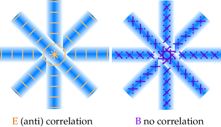
Figure 12: Temperature-polarization cross correlation. $E$-parity polarization perpendicular (parallel) to crests generates a tangential (radial) polarization field around hot spots. $B$-parity polarization does not correlate with temperature since the $\pm 45^{\circ}$ rotated contributions from oppositely directed modes cancel.

3.3.1 Large Angle Correlation Pattern

Consider first the large-angle scalar perturbations. Here the dominant source of correlated anisotropies is the temperature perturbation on the last scattering surface itself. The Doppler contributions can be up to half of the total contribution but as we have seen in §2.3 do not correlate with the quadrupole moment. Contributions after last scattering, while potentially strong in isocurvature models for example, also rapidly lose their correlation with the quadrupole at last scattering.

As we have seen, the temperature gradient associated with the scalar fluctuation makes the photon fluid flow from hot regions to cold initially. Around a point on a crest therefore the intensity peaks in the directions along the crest and falls off to the neighboring troughs. This corresponds to a polarization perpendicular to the crest (see Fig. 12). Around a point on a trough the polarization is parallel to the trough. As we superpose waves with different $\hat{\bf k}$ we find the pattern is tangential around hot spots and radial around cold spots ([Crittenden et al.] 1995). It is important to stress that the hot and cold spots refer only to the temperature component which is correlated with the polarization. The correlation increases at scales approaching the horizon at last scattering since the quadrupole anisotropy that generates polarization is caused by flows.

For the vectors, no temperature perturbations exist on the last scattering surface and again Doppler contributions do not correlate with the quadrupole. Thus the main correlations with the temperature will come from the quadrupole moment itself. The correlated signal is reduced since the strong $B$-contributions of vectors play no role. Hot spots occur in the direction $\theta=\pi/4$, $\phi=0$ where the hot lobe of the quadrupole is pointed at the observer (see Fig. 5). Here the $Q$ ($E$) component lies in the N-S direction perpendicular to the crest (see Fig. 6). Thus the pattern is tangential to hot spot, like scalars ([Hu & White] 1997). The signature peaks near the horizon at last scattering for reasons similar to the scalars.

For the tensors, both the temperature and polarization perturbations arise from the quadrupole moment, which fixes the sense of the main correlation. Hot spots and cold spots occur when the quadrupole lobe is pointed at the observer, $\theta=\pi/2$, $\phi=\pi/2$ and $3\pi/2$. The cold lobe and hence the polarization then points in the E-W direction. Unlike the scalars and vectors, the pattern will be mainly radial to hot spots ([Crittenden et al.] 1995). Again the polarization and hence the cross-correlation peaks near the horizon at last scattering since gravitational waves are frozen before horizon crossing ([Polnarev] 1985).

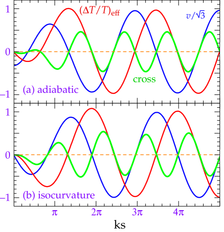
Figure 13: Time evolution of acoustic oscillations. The polarization is related to the flows $v$ (red) which form quadrupole anisotropies such that its product (green) with the effective temperature (blue) reflects the temperature-polarization cross correlation. As described in the text the adiabatic (a) and isocurvature (b) modes differ in the phase of the oscillation in all three quantities. Temperature and polarization are anticorrelated in both cases at early times or large scales $ks\ll 1$.

3.3.2 Small Angle Correlation Pattern

Until now we have implicitly assumed that the evolution of the perturbations plays a small role as is generally true for scales larger than the horizon at last scattering. Evolution plays an important role for small-scale scalar perturbations where there is enough time for sound to cross the perturbation before last scattering. The infall of the photon fluid into troughs compresses the fluid, increasing its density and temperature. For adiabatic fluctuations, this compression reverses the sign of the effective temperature perturbation when the sound horizon $s$ grows to be $ks\approx\pi/2$ (see Fig. 13a). This reverses the sign of the correlation with the quadrupole moment. Infall continues until the compression is so great that photon pressure reverses the flow when $ks\approx\pi$. Again the correlation reverses sign. This pattern of correlations and anticorrelations continues at twice the frequency of the acoustic oscillations themselves (see Fig. 13a). Of course the polarization is only generated at last scattering so the correlations and anticorrelations are a function of scale with sign changes at multiples of $\pi/2s_{*}$, where $s_{*}$ is the sound horizon at last scattering. As discussed in §3.2, these fluctuations project onto anisotropies as $\ell\sim kr$.

Any scalar fluctuation will obey a similar pattern that reflects the acoustic motions of the photon fluid. In particular, at the largest scales the $ks_{*}\ll\pi/2$, the polarization must be anticorrelated with the temperature because the fluid will always flow with the temperature gradient initially from hot to cold. However, where the sign reversals occur depend on the acoustic dynamics and so is a useful probe of the nature of the scalar perturbations, e.g. whether they are adiabatic or isocurvature ([Hu & White] 1996). In typical isocurvature models, the lack of initial temperature perturbations delays the acoustic oscillation by $\pi/2$ in phase so that correlations reverse at $ks_{*}=\pi$ (see Fig. 13b).

For the vector and tensor modes, strong evolution can introduce a small correlation with temperature fluctuations generated after last scattering. The effect is generally weak and model dependent and so we shall not consider it further here.

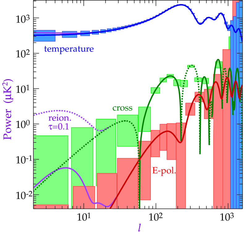
Figure 14: Temperature, polarization, and temperature-polarization cross correlation predictions and sensitivity of MAP for a fiducial model $\Omega_{0}=1$, $\Omega_{B}=0.1$, $h=0.5$ cold dark matter. The raw MAP satellite sensitivity (1 $\sigma$ errors on the recovered power spectrum binned in $\ell$) is approximated by noise weights of $w_{T}^{-1}=(0.11\mu K)^{2}$ for the temperature and $w_{P}^{-1}=(0.15\mu K)^{2}$ for the polarization and a FWHM beam of $0.25^{\circ}$. Note that errors between the spectra are correlated. While the reionized model (purple $\tau=0.1$) is impossible to distinguish from the fiducial model from temperature anisotropies alone, its effect on polarization is clearly visible at low $\ell$. Dashed lines for the temperature-polarization correlation represent anticorrelation. Animation (available at http://www.sns.ias.edu/$\sim$whu/polar/tauan.html): Variations in the spectra as $\tau$ is stepped from $0-1$.

4 Model Reconstruction

While it is clear how to compare theoretical predictions of a given model with observations, the reconstruction of a phenomenological model from the data is a more subtle issue. The basic problem is that in the CMB, we see the whole history of the evolution in redshift projected onto the two dimensional sky. The reconstruction of the evolutionary history of the universe might thus seem an ill-posed problem.

Fortunately, one needs only to assume the very basic properties of the cosmological model and the gravitational instability picture before useful information may be extracted. The simplest example is the combination of the amplitude of the temperature fluctuations, which reflect the conditions at horizon crossing, and large scale structure today. Another example is the acoustic peaks in the temperature which form a snapshot of conditions at last scattering on scales below the horizon at that time. In most models, the acoustic signature provides a wealth of information on cosmological parameters and structure formation ([Hu & White] 1996). Unfortunately, it does not directly tell us the behavior on the largest scales where important causal distinctions between models lie. Furthermore it may be absent in models with complex evolution on small scales such as cosmological defect models.

Here we shall consider how polarization information aids the reconstruction process by isolating the last scattering surface on large scales, and separating scalar, vector and tensor components. If and when these properties are determined, it will become possible to establish observationally the basic properties of the cosmological model such as the nature of the initial fluctuations, the mechanism of their generation, and the thermal history of the universe.

4.1 Last Scattering

The main reason why polarization is so useful to the reconstruction process is that (cosmologically) it can only be generated by Thomson scattering. The polarization spectrum of the CMB is thus a direct snapshot of conditions on the last scattering surface. Contrast this with temperature fluctuations which can be generated by changes in the metric fluctuations between last scattering and the present, such as those created by gravitational potential evolution. This is the reason why the mere detection of large-angle anisotropies by COBE did not rule out wide classes of models such as cosmological defects. To use the temperature anisotropies for the reconstruction problem, one must isolate features in the spectrum which can be associated with last scattering, or more generally, the universe at a known redshift.

Furthermore, the polarization spectrum has potential advantages even for extracting information from features that are also present in the temperature spectrum, e.g. the acoustic peaks. The polarization spectrum is generated by local quadrupole anisotropies alone whereas the temperature spectrum has comparable contributions from the local monopole and dipole as well as possible contributions between last scattering and the present. This property enhances the prominence of features (see Fig. 14) as does the fact that the scalar polarization has a relatively sharp projection due to the geometry (see §3.2). Unfortunately, these considerations are mitigated by the fact that the polarization amplitude is so much weaker than the temperature. With present day detectors, one needs to measure it in broad $\ell$-bands to increase the signal–to–noise (see Fig. 14 and Table 2).

4.2 Reionization

Since polarization directly probes the last scattering epoch the first thing we learn is when that occurred, i.e. what fraction of photons last scattered at $z\approx 1000$ when the universe recombined, and what fraction rescattered when the intergalactic medium reionized at $z_{\rm ri}\mathrel{\hbox to0.0pt{\lower 3.0pt\hbox{$\mathchar 536\relax$}\hss}\raise 2.0pt\hbox{$\mathchar 318\relax$}}5$.

Since rescattering erases fluctuations below the horizon scale and regenerates them only weakly ([Efstathiou] 1988), we already know from the reported excess (over COBE) of sub-degree scale anisotropy that the optical depth during the reionized epoch was $\tau\mathrel{\hbox to0.0pt{\lower 3.0pt\hbox{$\mathchar 536\relax$}\hss}\raise 2.0pt\hbox{$\mathchar 316\relax$}}1$ and hence

$$z_{\rm ri}\mathrel{\hbox to0.0pt{\lower 3.0pt\hbox{$\mathchar 536\relax$}\hss}\raise 2.0pt\hbox{$\mathchar 316\relax$}}100\left({\Omega_{0}h^{2}\over 0.25}\right)^{1/3}\left({\Omega_{B}h^{2}\over 0.0125}\right)^{-2/3}.$$ (11)

It is thus likely that our universe has the interesting property that both the recombination and reionization epoch are observable in the temperature and polarization spectrum.

Unfortunately for the temperature spectrum, at these low optical depths the main effect of reionization is an erasure of the primary anisotropies (from recombination) as $e^{-\tau}$. This occurs below the horizon at last scattering, since only on these scales has there been sufficient time to convert the originally isotropic temperature fluctuations into anisotropies. The uniform reduction of power at small scales has the same effect as a change in the overall normalization. For $z_{\rm ri}\sim 5$–20 the difference in the power spectrum is confined to large angles ($\ell<30$). Here the observations are limited by “cosmic variance”: the fact that we only have one sample of the sky and hence only $2\ell+1$ samples of any given multipole. Cosmic variance is the dominant source of uncertainty on the low-$\ell$ temperature spectrum in Fig. 14.

The same is not true for the polarization. As we have seen the polarization spectrum is very sensitive to the epoch of last scattering. More specifically, the location of its peak depends on the horizon size at last scattering and its height depends on the duration of last scattering ([Efstathiou] 1988). This signature is not cosmic variance limited until quite late reionization, though the combination of low optical depth and partial polarization will make it difficult to measure in practice (see Fig. 14 and Table 2). Optical depths of a few percent are potentially observable from the MAP satellite ([Zaldarriaga et al.] 1997) and of order unity from the POLAR experiment ([Keating et al.] 1997).

On the other hand, these considerations imply that the interesting polarization signatures from recombination will not be completely obscured by reionization. We turn to these now.

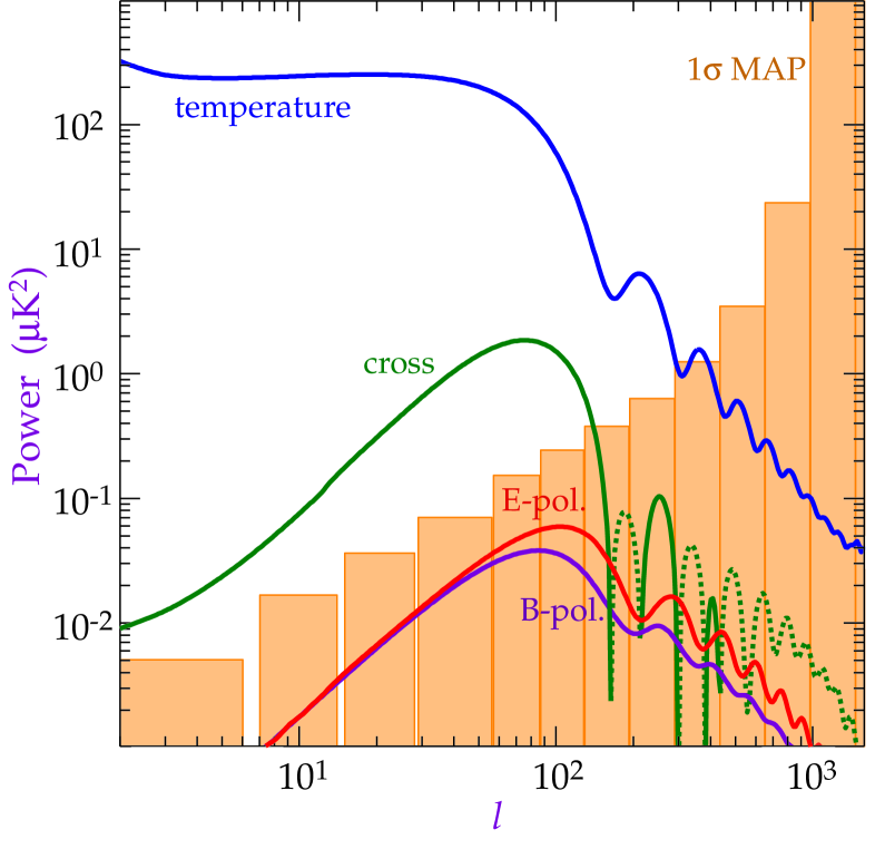
Figure 15: Tensor power spectra. The tensor temperature, temperature-cross-polarization, $E$-mode, and $B$-mode polarization for a scale invariant intial spectrum of tensors with $\Omega_{0}=1.0$, $\Omega_{B}=0.1$ and $h=0.5$. The normalization has been artificially set (high) to have the same quadrupole as the scalar spectrum of Fig. 14. Also shown is the MAP $1\sigma$ upper limits on the $B$-mode due to noise, i.e. assuming no signal, showing that higher sensitivity will likely be necessary to obtain a significant detection of $B$-polarization from tensors.

4.3 Scalars, Vectors, & Tensors

There are three types of fluctuations: scalars, vectors and tensors, and four observables: the temperature, $E$-mode, $B$-mode, and temperature cross polarization power spectra. The CMB thus provides sufficient information to separate these contributions, which in turn can tell us about the generation mechanism for fluctuations in the early universe (see §4.5).

Ignoring for the moment the question of foregrounds, to which we turn in §5.2, if the $E$-mode polarization greatly exceeds the $B$-mode then scalar fluctuations dominate the anisotropy. Conversely if the $B$-mode is greater than the $E$-mode, then vectors dominate. If tensors dominate, then the $E$ and $B$ are comparable (see Fig. 15). These statements are independent of the dynamics and underlying spectrum of the perturbations themselves.

The causal constraint on the generation of a quadrupole moment (and hence the polarization) introduces further distinctions. It tells us that the polarization peaks around the scale the horizon subtends at last scattering. This is about a degree in a flat universe and scales with the angular diameter distance to last scattering. Geometric projection tells us that the low-$\ell$ tails of the polarization can fall no faster than $\ell^{6}$, $\ell^{4}$ and $\ell^{2}$ for scalars, vectors and tensors (see §3.2). The cross spectrum falls no more rapidly than $\ell^{4}$ for each. We shall see below that these are the predicted slopes of an isocurvature model.

Furthermore, causality sets the scale that separates the large and small angle temperature-polarization correlation pattern. Well above this scale, scalar and vector fluctuations should show anticorrelation (tangential around hot spots) whereas tensor perturbations should show correlations (radial around hot spots).

Of course one must use measurements at small enough angular scales that reionization is not a source of confusion and one must understand the contamination from foregrounds extremely well. The latter is especially true at large angles where the polarization amplitude decreases rapidly.

4.4 Adiabatic vs. Isocurvature Perturbations

The scalar component is interesting to isolate since it alone is responsible for large scale structure formation. There remain however two possibilities. Density fluctuations could be present initially. This represents the adiabatic mode. Alternately, they can be generated from stresses in the matter which causally push matter around. This represents the isocurvature mode.

The presence or absence of density perturbations above the horizon at last scattering is crucial for the features in both the temperature and polarization power spectrum. As we have seen in §3.3.1, it has as strong effect on the phase of the acoustic oscillation. In a typical isocurvature model, the phase is delayed by $\pi/2$ moving structure in the temperature spectrum to smaller angles (see Fig. 13). Consistency checks exist in the $E$-polarization and cross spectrum which should be out of phase with the temperature spectrum and oscillating at twice the frequency of the temperature respectively. However, if the stresses are set up sufficiently carefully, this acoustic phase test can be evaded by an isocurvature model ([Turok] 1996). Perhaps more importantly, acoustic features can be washed out in isocurvature models with complicated small scale dynamics to force the acoustic oscillation, as in many defect models ([Albrecht et al.] 1996).

Even in these cases, the polarization carries a robust signature of isocurvature fluctuations. The polarization isolates the last scattering surface and eliminates any source of confusion from the epoch between last scattering and the present. In particular, the delayed generation of density perturbations in these models implies a steep decline in the polarization above the angle subtended by the horizon at last scattering. The polarization power thus hits the asymptotic limits given in the previous section in contrast to the adiabatic power spectra shown in Fig. 14 which have more power at large angles. To be more specific, if the $E$-power spectrum falls off as $\ell^{6}$ and or the cross spectrum as $\ell^{4}$, then the initial fluctuations are isocurvature in nature (or an adiabatic model with a large spectral index, which is highly constrained by COBE).

Of course measuring a steeply falling spectrum is difficult in practice. Perhaps more easily measured is the first feature in the adiabatic $E$-polarization spectrum at twice the angular scale of the first temperature peak and the first sign crossing of the correlation at even larger scales. Since isocurvature models must be pushed to the causal limit to generate these features, their observation would provide good evidence for the adiabatic nature of the initial fluctuations ([Hu, Spergel & White] 1997).

4.5 Inflation vs. Defects

One would like to know not only the nature of the fluctuations, but also the means by which they are generated. We assume of course that they are not merely placed by fiat in the initial conditions. Let us first divide the possibilities into broad classes. In fact, the distinction between isocurvature and adiabatic fluctuations is operationally the same as the distinction between conventional causal sources (e.g. defects) and those generated by a period of superluminal expansion in the early universe (i.e. inflation). It can be shown that inflation is the only causal mechanism for generating superhorizon size density (curvature) fluctuations ([Liddle] 1995). Since the slope of the power spectrum in $E$ can be traced directly to the presence of “superhorizon size” temperature, and hence curvature, fluctuations at last scattering, it represents a “test” of inflation ([Hu & White] 1997, [Spergel & Zaldarriaga] 1997). The acoustic phase test, either in the temperature or polarization, represents a marginally less robust test that should be easily observable if the former fails to be.

These tests, while interesting, do not tell us anything about the detailed physics that generates the fluctuations. Once a distinction is made between the two possibilities one would like to learn about the mechanism for generating the fluctuations in more detail. For example in the inflationary case there is a well known test of single-field slow-roll inflation which can be improved by using polarization information. In principle, inflation generates both scalar and tensor anisotropies. If we assume that the two spectra come from a single underlying inflationary potential their amplitudes and slopes are not independent. This leads to an algebraic consistency relation between the ratio of the tensor and scalar perturbation spectra and the tensor spectral index. However information on the tensor contribution to the spectrum is limited by cosmic variance and is easily confused with other effects such as those of a cosmological constant or tilt of the initial spectrum. By using polarization information much smaller ratios of tensor to scalar perturbations may be probed, with more accuracy, and the test refined (see [Zaldarriaga et al.] 1997 for details). In principle, this extra information may also allow one to reconstruct the low order derivatives of the inflaton potential.

Similar considerations apply to causal generation of fluctuations without inflation. Two possibilities are a model with “passive evolution” where initial stress fluctuations move matter around and “active evolution” where exotic but causal physics continually generates stress-energy perturbations inside the horizon. All cosmological defect models bear aspects of the latter class. The hallmark of an active generation mechanism is the presence of vector modes. Vector modes decay with the expansion so in a passive model they would no longer be present by recombination. Detection of (cosmological) vector modes would be strong evidence for defect models. Polarization is useful since it provides a unique signature of vector modes in the dominance of the $B$-mode polarization ([Hu & White] 1997). Its level for several specific defect models is given in [Seljak, Pen, Turok] (1997).

5 Phenomenology

5.1 Observations

While the theoretical case for observing polarization is strong, it is a difficult experimental task to observe signals of the low level of several $\mu$K and below. Nonetheless, polarization experiments have one potential advantage over temperature anisotropy experiments. They can reduce atmospheric emission effects by differencing the polarization states on the same patch of sky instead of physically chopping between different angles on the sky since atmospheric emission is thought to be nearly unpolarized (see §5.2). However, to be successful an experiment must overcome a number of systematic effects, many of which are discussed in [Keating et al.] (1997). It must at least balance the sensitivity of the instrument to the orthogonal polarization channels (including the far side lobes) to nearly 8 orders of magnitude. Multiple levels of switching and a very careful design are minimum requirements.

To date the experimental upper limits on polarization of the CMB have been at least an order of magnitude larger than the theoretical expectations. The original polarization limits go back to Penzias & Wilson (1965) who set a limit of 10% on the polarization of the CMB. There have been several subsequent upper limits which have now reached the level of $\sim 20\mu$K (see Tab. 1), about a factor of 5–10 above the predicted levels for popular models (see Tab. 2).

Reference	Frequency (GHz)	Ang. Scale	$\Delta T(\mu$K)	(CL)
[Penzias & Wilson] (1965)	4.0	–	$10^{5}$	95%
[Nanos] (1979)	9.3	$15^{\circ}$ beam	$2\times 10^{3}$	90%
[Caderni et al.] (1978)	100-600	$0.5^{\circ}\mathrel{\hbox to0.0pt{\lower 3.0pt\hbox{$\mathchar 536\relax$}\hss}\raise 2.0pt\hbox{$\mathchar 316\relax$}}\theta\mathrel{\hbox to0.0pt{\lower 3.0pt\hbox{$\mathchar 536\relax$}\hss}\raise 2.0pt\hbox{$\mathchar 316\relax$}}40^{\circ}$	$2\times 10^{3}(40^{\circ}/\theta)^{1/2}$	65%
[Lubin & Smoot] (1981)	33	$\ell\la 3$	$200$	95%
[Partridge et al.] (1988)	5	$1^{\prime}\mathrel{\hbox to0.0pt{\lower 3.0pt\hbox{$\mathchar 536\relax$}\hss}\raise 2.0pt\hbox{$\mathchar 316\relax$}}\theta\mathrel{\hbox to0.0pt{\lower 3.0pt\hbox{$\mathchar 536\relax$}\hss}\raise 2.0pt\hbox{$\mathchar 316\relax$}}3^{\prime}$	$100$	95%
[Wollack et al.] (1993)	26-36	$50\mathrel{\hbox to0.0pt{\lower 3.0pt\hbox{$\mathchar 536\relax$}\hss}\raise 2.0pt\hbox{$\mathchar 316\relax$}}\ell\mathrel{\hbox to0.0pt{\lower 3.0pt\hbox{$\mathchar 536\relax$}\hss}\raise 2.0pt\hbox{$\mathchar 316\relax$}}100$	$25$	95%
[Netterfield et al.] (1995)	26-46	$50\mathrel{\hbox to0.0pt{\lower 3.0pt\hbox{$\mathchar 536\relax$}\hss}\raise 2.0pt\hbox{$\mathchar 316\relax$}}\ell\mathrel{\hbox to0.0pt{\lower 3.0pt\hbox{$\mathchar 536\relax$}\hss}\raise 2.0pt\hbox{$\mathchar 316\relax$}}100$	$16$	95%

Table 1: Experimental upper limits on the polarization of the CMB. The values are converted from the quoted $\Delta T/T$ by multiplying by $T=2.728$K, thus these numbers only approximate the bandpowers used in Tab. 2.

Cosmological Parameters				$\ell$: 2–20 ($\mu$K)			$\ell$: 100-200 ($\mu$K)			$\ell$: 700–1000 ($\mu$K)
$\Omega_{0}$	$\Omega_{\rm B}$	$z_{\rm ri}$	$T/S$	$E$	$TE$	$B$	$E$	$TE$	$B$	$E$	$TE$	$B$
1.0	0.05	0	0	0.02	($-$)0.42	0	0.68	(+)3.6	0	3.7	(+)4.8	0
1.0	0.10	0	0	0.017	($-$)0.40	0	0.71	(+)4.2	0	3.4	(+)3.3	0
1.0	0.05	5	0	0.03	($-$)0.59	0	0.68	(+)3.6	0	3.7	(+)4.8	0
1.0	0.05	10	0	0.06	($-$)0.78	0	0.68	(+)3.6	0	3.6	(+)4.8	0
1.0	0.05	20	0	0.14	($-$)1.1	0	0.66	(+)3.5	0	3.5	(+)4.7	0
1.0	0.05	0	0.1	0.02	($-$)0.40	0.01	0.65	(+)3.4	0.05	3.5	(+)4.6	0.01
$0.4_{K}$	0.05	0.1	0	0.01	($-$)0.18	0	0.44	(+)2.3	0	2.8	(+)5.5	0
$0.4_{\Lambda}$	0.05	0	0	0.02	($-$)0.37	0	0.65	(+)4.0	0	4.1	(+)6.4	0

Table 2: Bandpowers for a selection of cosmological models all with $h=0.5$ and scale invariant spectra save for the $T/S=0.1$ model where $T/S=7(1-n_{s})$. The low-$\Omega_{0}$ models are indicated as $0.4_{K}$ for the open model and $0.4_{\Lambda}$ for the model with $\Omega_{\Lambda}=1-\Omega_{0}=0.6$. The bandpower is defined in units of the COBE quadrupole over the range of $\ell$ indicated. The sign of the cross correlation is indicated in parentheses and note that the band averaged signal may be suppressed from cancellation of correlated and anticorrelated angular regimes.

5.2 Foregrounds

Given that the amplitude of the polarization is so small the question of foregrounds is even more important than for the temperature anisotropy. Unfortunately, the level and structure of the various foreground polarization in the CMB frequency bands is currently not well known. We review some of the observations in the adjacent radio and IR bands (a more complete discussion can be found in [Keating et al.] 1997). Atmospheric emission is believed to be negligibly polarized ([Keating et al.] 1997), leaving the main astrophysical foregrounds: free-free, synchrotron, dust, and point source emissions. Of these the most important foreground is synchrotron emission.

Free-free emission (bremsstrahlung) is intrinsically unpolarized ([Rybicki & Lightman] 1979) but can be partially polarized by Thomson scattering within the HII region. This small effect is not expected to polarize the emission by more than 10% ([Keating et al.] 1997). The emission is larger at low frequencies but is not expected to dominate the polarization at any frequency.

The polarization of dust is not well known. In principle, emission from dust particles could be highly polarized, however [Hildebrand & Dragovan] (1995) find that in their observations the majority of dust is polarized at the $\approx 2\%$ level at $100\mu$m with a small fraction of regions approaching $10\%$ polarization. Moreover [Keating et al.] (1997) show that even at 100% polarization, extrapolation of the IRAS 100$\mu$m map with the COBE FIRAS index shows that dust emission is negligible below $80$GHz. At higher frequencies it will become the dominant foreground.

Radio point sources are polarized due to synchrotron emission at $<20\%$ level. For large angle experiments, the random contribution from point sources will contribute negligibly, but may be of more concern for the upcoming satellite missions.

Galactic synchrotron emission is the major concern. It is potentially highly polarized with the fraction dependent on the spectral index and depolarization from Faraday rotation and non-uniform magnetic fields. The level of polarization is expected to lie between 10%-75% of a total intensity which itself is approximately $50\mu$K at $30$GHz. This estimate follows from extrapolating the [Brouw & Spoelstra] (1976) measurements at 1411 MHz with an index of $T\propto\nu^{-3}$.

Due to their different spectral indices, the minimum in the foreground polarization, like the temperature, lies near 100GHz. For full sky measurements, since synchrotron emission is more highly polarized than dust, the optimum frequency at which to measure intrinsic (CMB) polarization is slightly higher than for the anisotropy. Over small regions of the sky where one or the other of the foregrounds is known a priori to be absent the optimum frequency would clearly be different. However as with anisotropy measurements, with multifrequency coverage, polarized foregrounds can be removed.

It is also interesting to consider whether the spatial as well as frequency signature of the polarization can be used to separate foregrounds. Using angular power spectra for the spatial properties of the foregrounds is a simple generalization of methods already used in anisotropy work. For instance, in the case of synchotron emission, if the spatial correlation in the polarization follows that of the temperature itself, the relative contamination will decrease on smaller angular scales due to its diffuse nature. Furthermore the peak of the cosmic signal in polarization occurs at even smaller angular scales than for the anisotropy.

One could attempt to exploit the additional properties of polarization, such as its $E$- and $B$-mode nature. We mentioned above that in a wide class of models where scalars dominate on small angular scales, the polarization is predicted to be dominantly $E$-mode ([Kamionkowski et al.] 1997 [Zaldarriaga & Seljak] 1997). [Seljak] (1997) suggests that one could use this to help eliminate foreground contamination by “vetoing” on areas of $B$-mode signal. However in general one does not expect that the foregrounds will have equal $E$- and $B$-mode contribution, so while this extra information is valuable, its use as a foreground monitor can be compromised in certain circumstances. Specifically, if a correlation exists between the direction of polarization and the rate of change (curvature) of its amplitude, the foreground will populate the two modes unequally. Two simple examples: either radial or tangential polarization around a source with the amplitude of the polarization dropping off with radius, or polarization parallel or perpendicular to a “jet” whose amplitude drops along the jet axis. Both examples would give predominantly $E$-mode polarization.

5.3 Data Analysis

Several authors have addressed the question of the optimal estimators of the polarization power spectra from high sensitivity, all-sky maps of the polarization. They suggest that one calculate the coefficients of the expansion in spin-2 spherical harmonics and then form quadratic estimators of the power spectrum, as the average of the squares of the coefficients over $m$, corrected for noise bias as in the example of Fig. 14.

We shall return to consider this below, however before such maps are obtained we would like to know how to analyze ground based polarization data. These data are likely to consist of $Q$ and $U$ measurements from tens or perhaps hundreds of pointings, convolved with an approximately gaussian beam on some angular scale. How can we use this data to provide constraints or measurements of the electric and magnetic power spectra, presumably averaged across bands in $\ell$?

For a small number of points, the simplest and most powerful way to obtain the power spectrum is to perform a likelihood analysis of the data. The likelihood function encodes all of the information in the measurement and can be modified to correctly account for non-uniform noise, sky coverage, foreground subtraction and correlations between measurements. Operationally, one computes the probability of obtaining the measured points $Q_{i}\equiv Q(\hat{\bf n}_{i})$ and $U_{i}\equiv U(\hat{\bf n}_{i})$ assuming a given “theory” (including a model for foregrounds and detector noise) and maximizes the likelihood over the theories. For our purposes, the theories could be given simply by the polarization bandpowers in $E$ and $B$ for example, or could be a more “realistic” model such as CDM with a given reionization history. The confidence levels on the parameters are obtained as moments of the likelihood function in the usual way. Such an approach also allows one to generalize the analysis to include temperature information (for the cross correlation) if it becomes available.

Assuming that the fluctuations are gaussian, the likelihood function is given in terms of the data and the correlation function of $Q$ and $U$ for any pair of the $n$ data points. The calculation of this correlation function is straightforward, and [Kamionkowski et al.] (1997) discuss the problem extensively. Let us assume that we are fitting only one component or have only one frequency channel. The generalization to multiple frequencies with a model for the foreground is also straightforward. We shall also assume for notational simplicity that we are fitting only to polarization data, though again the generalization to include temperature data is straightforward. The construction is as follows. We define a data vector which contains the $Q$ and $U$ information referenced to a particular coordinate system (in principle this coordinate system could change between different subsets of the data). Call this data vector

$$D=(Q_{1},U_{1},\ldots,Q_{n},U_{n}),$$ (12)

which has $N=2n$ components. We can construct the likelihood of obtaining the data given a theory once we know the correlation matrix $C_{IJ}$:

$${\cal L}(D|T)\propto{1\over\sqrt{\det{C}}}\exp\left[-{1\over 2}D_{I}C^{-1}_{IJ}D_{J}\right]$$ (13)

All of the theory information is encoded in $C_{IJ}=C_{IJ}^{\rm th}+N_{IJ}$, where $N_{IJ}$ is the noise correlation matrix, to be provided by the experiment, and $C_{IJ}^{\rm th}$ is a function of the theory parameters.

All that remains is to compute each element of $C_{IJ}^{\rm th}$ for a given theory. Consider a pair of points $i$ and $j$ corresponding to 4 entries of our data vector $D_{I}$. Following [Kamionkowski et al.] (1997), define $Q^{\prime}$ and $U^{\prime}$ as the components of the polarization in a new coordinate system, where the great arc connecting $\hat{\bf n}_{1}$ and $\hat{\bf n}_{2}$ runs along the equator. Expressions for $\langle Q^{\prime}Q^{\prime}\rangle$ and $\langle U^{\prime}U^{\prime}\rangle$ in terms of the $E$ and $B$ angular power follow directly from the definitions of these spectra and the spin-weighted spherical harmonics. They can be found in [Kamionkowski et al.] (1997) [their Eqs. (5.9,5.10)]. They also give the flat sky limit of these equations. Knowing the angle $\phi_{ij}$ about $\hat{\bf n}_{i}$ through which we must rotate our primed coordinate system to return to the system in which our data is defined we can write

$$Q_{i} = Q_{i}^{\prime}\cos 2\phi_{ij}+U_{i}^{\prime}\sin 2\phi_{ij}$$

$$U_{i} = Q_{i}^{\prime}\sin 2\phi_{ij}-U_{i}^{\prime}\cos 2\phi_{ij}$$ (14)

and similarly for the $j$th element. Thus using the known expressions for $\langle Q^{\prime}Q^{\prime}\rangle$ and $\langle U^{\prime}U^{\prime}\rangle$ we can calculate $\langle Q_{i}Q_{j}\rangle$, $\langle U_{i}U_{j}\rangle$, $\langle Q_{i}U_{j}\rangle$ and $\langle U_{i}Q_{j}\rangle$ for the $i$th and $j$th pixel and thus all of the elements of $C_{IJ}^{\rm th}$. Substitution of $C_{IJ}^{\rm th}$ into Eq. (13) allows one to obtain limits on any theory given the data.

Finally let us note that the method outlined here is completely general and thus can be applied also the the high-sensitivity, all-sky maps which would result from satellite experiments. For these experiments, the large volume of data is however an issue in the analysis pipeline design, as has been addressed by several authors. The generalization of the above analysis procedure to include filtering and compression is straightforward, and directly analogous to the case of anisotropy, so we will not discuss it explicitly here.

6 Future Prospects

Following a hiatus of some years, experimental efforts to detect CMB polarization are now underway. At the large angular scale, an experiment based in Wisconsin ([Keating et al.] 1997) plans to make a $30$GHz measurement of polarization on $7^{\circ}$ angular scales with a sensitivity of a few $\mu$K per pixel. The main goal of the experiment would be to look for the signature of reionization (see Fig. 14). Several groups are currently considering measuring the signature at smaller scales from recombination.

The MAP and Planck missions also plan to measure polarization. Because of their all sky nature these missions will be the first to be able to measure the polarization power spectrum and temperature cross correlation with reasonable spectral sensitivity. We show an example of the sensitivity to the which MAP should nominally obtain in the absence of foregrounds and systematic effects in Fig. 14. As can be seen, MAP should certainly detect the $E$-mode of polarization at medium angular scales, and obtain a significant detection of the temperature polarization cross-correlation. These signatures can be useful for separating adiabatic and isocurvature models of structure formation as we have seen in §4.

However the detailed study of the polarization power spectrum will require the improved sensitivity and expanded frequency coverage of Planck for detailed features and foreground removal respectively. Planck will have the sensitivity to make a measurement of the large-angle polarization predicted in CDM models, regardless of the epoch of reionization if foreground contamination can be removed. Likewise, it can potentially measure small levels of $B$-mode polarization. The separation of the $E$ and $B$ modes is of course crucial for the isolation of scalar, vector and tensor modes and so the reconstruction problem in general.

Clearly, the polarization spectrum represents another gold mine of information in the CMB. Though significant challenges will have to be overcome, the prospects for its detection are bright.

Acknowledgments: We thank D. Eisenstein, S. Staggs, M. Tegmark, P. Timbie and M. Zaldarriaga for useful discussions. W.H. acknowledges support from the W.M. Keck foundation.

whu@ias.edu

http://www.sns.ias.edu/$\sim$whu/polar/polar.html

References

- [Albrecht et al.] Albrecht, A., Coulson, D., Ferreira, P. & Magueijo, J., 1996, Phys. Rev. Lett., 76, 1413. [astro-ph/9505030]
- [Bond & Efstathiou] Bond, J.R. & Efstathiou, G., 1984, ApJ Lett, 285, L45.
- [Brouw & Spoelstra] Brouw, W.N. & Spoelstra, T.A. 1976, A&AS, 26, 129.
- [Caderni et al.] Caderni, N., Fabbri, R., Melchiorri, B., Melchiorri, F., Natale, V., 1978, Phys. Rev. D, 17, 1901.
- [Chandrasekhar] Chandrasekhar, S., 1960, Radiative Transfer, Dover, New York.
- [Crittenden et al.] Crittenden, R.G., Coulson, D. & Turok, N.G., 1995, Phys. Rev. D, 52, 5402. [astro-ph/9411107]
- [Efstathiou] Efstathiou, G., 1988, in Large Scale Motions in the Universe: A Vatican Study Week, eds. V.C. Rubin & G.V. Coyne, Princeton U. Press, Princeton.
- [Hildebrand & Dragovan] Hildebrand, R. & Dragovan M., 1995, ApJ, 450, 663.
- [Hu, Spergel & White] Hu, W., Spergel, D.N. & White, M., 1997, Phys. Rev. D., 55, 3288. [astro-ph/9605193]
- [Hu & White] Hu, W. & White, M., 1996, ApJ, 479, 568. [astro-ph/9602019]
- [Hu & White] Hu, W. & White, M., 1997, Phys. Rev. D (in press). [astro-ph/9702170]
- [Kamionkowski et al.] Kamionkowski, M., Kosowsky, A., & Stebbins, A., 1997, Phys. Rev. D (in press). [astro-ph/9611125]
- [Kaiser] Kaiser, N., 1983, MNRAS, 202, 1169.
- [Keating et al.] Keating, B., Timbie, P., Polnarev, A., & Steinberger, J., submitted to ApJ.
- [Liddle] Liddle, A. 1995, Phys. Rev. D., 51, 5347.
- [Lubin & Smoot] Lubin, P. & Smoot, G., 1981, ApJ Lett., 245, L1.
- [Nanos] Nanos, G.P., 1979, ApJ, 232, 341.
- [Netterfield et al.] Netterfield, C.B. et al., 1995, ApJ, 474, L69. [astro-ph/9411035]
- [Newman & Penrose] Newman, E. & Penrose, R., 1966, J. Math Phys., 7, 863.
- [Partridge et al.] Partridge, B., et al., 1988, Nature, 331, 146.
- [Penzias & Wilson] Penzias, A.A. & Wilson, R.W., 1965 ApJ, 142, 419
- [Polnarev] Polnarev, A.G., 1985, Sov. Astron., 29, 607.
- [Rybicki & Lightman] Rybicki, G.B., Lightman, A., 1979, Radiative Processes in Astrophysics, New York, Wiley
- [Sachs & Wolfe] Sachs, R.K. & Wolfe, A.M., 1967 ApJ, 147, 73.
- [Seljak] Seljak, U. 1997 ApJ, 482, 6. [astro-ph/9608131]
- [Seljak, Pen, Turok] Seljak, U., Pen, U., & Turok, N., 1997, preprint. [astro-ph/9704231]
- [Spergel & Zaldarriaga] Spergel, D.N. & Zaldarriaga, M., 1997, preprint. [astro-ph/9705182]
- [Turok] Turok, N.G., 1996, Phys. Rev. Lett, 77, 4138. [astro-ph/9607109]
- [Wollack et al.] Wollack, E.J. et al., 1993, ApJ, 419, L49.
- [Zaldarriaga & Seljak] Zaldarriaga, M. & Seljak, U. 1997, Phys. Rev. D 55 1830. [astro-ph/9609170]
- [Zaldarriaga et al.] Zaldarriaga, M., Spergel, D.N., & Seljak, U., 1997, preprint. [astro-ph/9702157]