On the Effective Spatial Separations
in the Clustering of Faint Galaxies

Abstract

Several recent measurements have been made of the angular correlation function $w(\theta,m)$ of faint galaxies in deep surveys (e.g., in the Hubble Deep Field, HDF). Are the measured correlations indicative of gravitational growth of primordial perturbations or of the relationship between galaxies and (dark matter dominated) galaxy haloes? A first step in answering this question is to determine the typical spatial separations of galaxies whose spatial correlations, $\xi(r,z),$ contribute most of the angular correlation.

The median spatial separation of galaxy pairs contributing to a fraction $p$ of the angular correlation signal in a galaxy survey is denoted by $r_{\mbox{\rm\small eff}}^{p}$ (§3) and compared with the perpendicular distance, $r_{\perp},$ at the median redshift, $z_{\mbox{\rm\small med}}$, of the galaxies. Over a wide range in spatial correlation growth rates $\epsilon$ and median redshifts, $r_{\mbox{\rm\small eff}}^{50\%}$ is no more than about twice the value of $r_{\perp},$ while $r_{\mbox{\rm\small eff}}^{90\%}$ is typically four times $r_{\perp}.$

Values of $r_{\mbox{\rm\small eff}}^{p}$ for redshift distributions representative of recent surveys indicate that many angular correlation measurements correspond to spatial correlations at comoving length scales well below 1$h^{-1}$ Mpc. For $\Omega_{0}=1$ and $\lambda_{0}=0$, the correlation signal at 4^′′ predominant in the [Villumsen et al.] (1996) estimates of $w(\theta,m)$ for faint HDF galaxies corresponds to $r_{\mbox{\rm\small eff}}^{50\%}$ (HDF) $\approx 40h^{-1}$ kpc; other cosmologies and angles up to 10^′′ can increase this to $r_{\mbox{\rm\small eff}}^{50\%}$ (HDF) $\,\lower 2.58334pt\hbox{$\buildrel<\over{\sim}$}\,200h^{-1}$ kpc. The proper separations are $(1+z)$ times smaller, where $1\,\lower 2.58334pt\hbox{$\buildrel<\over{\sim}$}\,z\,\lower 2.58334pt\hbox{$\buildrel<\over{\sim}$}\,2.$

These scales are small: the faint galaxy angular correlation measurements are at scales where halo and/or galaxy existence, let alone interactions, may modify the spatial correlation function. These measurements could be used to probe the radial extent of haloes at high redshift.

Division of Theoretical Astrophysics, National Astronomical Observatory, Mitaka, Tokyo 181, Japan
Email: roukema@iap.fr and URA CNRS 1280, Observatoire de Strasbourg, 11 rue de l’Université, 67000 Strasbourg, France
Royal Greenwich Observatory, Madingley Road, Cambridge CB3 0EZ, UK
Email: dvg@astro.u-strasbg.fr dvg@ast.cam.ac.uk

Subject headings: cosmology: theory—galaxies: formation—galaxies: clusters: general—galaxies: distribution—cosmology: observations

1 INTRODUCTION

The growth of primordial density fluctuations into galaxies and clusters of galaxies is an essential element of understanding how structure forms in the Universe. A common way to statistically represent this structure from observed galaxies is to calculate the two-point auto-correlation function, $\xi(r,z),$ which can be approximately parametrised as a power law (in spatial separation of galaxy pairs) which increases in amplitude as a function of time, according to a single parameter $\epsilon,$ (e.g., [Groth & Peebles] 1977):

$$\xi(r,z)=(r_{0}/r)^{\gamma}(1+z)^{-(3+\epsilon-\gamma)}$$ (1)

where $r$ and $r_{0}$ are expressed in comoving coordinates and $\gamma$ represents the approach to homogeneity at larger length scales.

Observed values are typically $r_{0}\approx 5h^{-1}$ Mpc and $\gamma\approx 1{\cdot}7-1{\cdot}8$ (e.g., [Davis & Peebles] 1983; [Loveday et al.] 1992) for the low redshift general galaxy population. [Davis & Peebles]’ (1983) analysis is consistent with this power law on scales $10h^{-1}$ kpc$\,\lower 2.58334pt\hbox{$\buildrel<\over{\sim}$}\,r\,\lower 2.58334pt\hbox{$\buildrel<\over{\sim}$}\,10h^{-1}$ Mpc, though the correlations appear somewhat stronger at the small scale end (but noisy).

[Loveday et al.] (1992) find their power law fit to $\xi$ of the Stromlo-APM redshift survey to be valid over $200h^{-1}$ kpc$\,\lower 2.58334pt\hbox{$\buildrel<\over{\sim}$}\,r\,\lower 2.58334pt\hbox{$\buildrel<\over{\sim}$}\,20h^{-1}$ Mpc.

Direct estimates of the evolution in this power law at low $z_{\mbox{\rm\small med}}$ (median redshifts) include $\epsilon=1{\cdot}6\pm 0{\cdot}5$ ([Warren et al.] 1993, $z_{\mbox{\rm\small med}}$$=0{\cdot}4$), $\epsilon=-2{\cdot}0\pm 2{\cdot}7$ ([Cole et al.] 1994, $z_{\mbox{\rm\small med}}$$=0{\cdot}16$) and $\epsilon=0{\cdot}8^{+1.0}_{-1.3}$ ([Shepherd et al.] 1996, $z_{\mbox{\rm\small med}}$$=0{\cdot}36$). However, consideration of galaxies as a single population, i.e., adoption of $r_{0}=5{\cdot}0h^{-1}$ Mpc and the median redshift ($c$$z_{\mbox{\rm\small med}}$$=15,200$ km s^-1) of the Stromlo-APM survey ([Loveday et al.] 1992, 1995) for comparison with the higher $z_{\mbox{\rm\small med}}$$=0{\cdot}56$ CFRS estimate of $\xi$ (Le Fèvre et al. 1996, [CFRS-VIII]) would imply that $\epsilon=2{\cdot}8$ (cf. §4.1(3), [CFRS-VIII]).

This latter value of $\epsilon$ is considerably higher than expected either for clustering fixed in comoving coordinates ($\epsilon=\gamma-3\approx-1{\cdot}2$, so that the index in Eq. 1 is zero); clustering fixed in proper coordinates on small scales [“stable clustering”, $\epsilon=0$, since the numbers of “clusters” changes by $(1+z)^{3}$ and the number of galaxy pairs by $(1+z)^{6}$, the factor in Eq. 1 for $r$ in proper coordinates is $(1+z)^{-3}$]; or linear growth of density perturbations in an Einstein-de Sitter universe ($\epsilon=\gamma-1\approx 0{\cdot}8$). [Note also that the high $z$ behaviour of $\xi$ may be different (e.g., [Ogawa et al.] 1997).]

A lower value of $\epsilon$ could be justified by hypothesising major changes in visible galaxy populations from low to high redshifts, as suggested by indications of colour dependence in the correlation function (e.g., [Infante & Pritchet] 1995).

The validity or otherwise of the high observational estimates of $\epsilon$ or of major changes in the general galaxy population is not the subject of this article. In fact, as will be defined and seen below, the parameter of interest $r_{\mbox{\rm\small eff}}^{p}$ is only weakly sensitive to $\epsilon.$

The motivation for this article stems from the attempts to indirectly measure the dependence of $\xi$ on $z.$ Since estimation of spectroscopic redshifts requires many more photons than the photometric detection of a galaxy, the projection of $\xi$ onto the celestial sphere, i.e., the angular correlation function, $w(\theta,m),$ for angle $\theta$ and survey “limiting apparent magnitude” $m,$ can be more easily measured than $\xi.$ This means that $\xi$ can be effectively measured at larger redshifts than is obtainable in redshift surveys—but at the cost of having to deduce $\xi$ from its sky projection.

Hence, investigation of the $z$ dependence of $\xi$ can be carried out to larger redshifts by measuring $w$ rather than $\xi.$ Many estimates of the amplitude of $w(\theta,m)$ of faint galaxies in faint magnitude (“deep”) small angle (a few square arcminutes, “pencil beam”, or up to a few square degrees) surveys have been carried out recently (e.g., [Efstathiou et al.] 1991; [Neuschaefer et al.] 1991; [Pritchet & Infante] 1992; [Couch et al.] 1993; [Roukema & Peterson] 1994; [Infante & Pritchet] 1995; [Brainerd et al.] 1995). These angular correlations are usually interpreted by integrating $\xi(r,z)$ (Eq. 1) over an appropriate domain in $z-u$ space (see Eq. 2).

The resulting values of $\epsilon,$ or hypotheses about how population transitions might justify change in the value of $r_{0}$ as a function of $z,$ are generally discussed, and an indication of the scale of galaxy pair separations is sometimes indicated by $r_{\perp}\equiv d_{\mbox{\rm\small prop}}\theta\equiv r(z,u=0)$ (for $r$ in comoving coordinates; $u$ is redshift separation of a galaxy pair at mean redshift $z$, defined below for Eq. 2) at the median redshift, $z_{\mbox{\rm\small med}}$, of the redshift distribution of the galaxy sample.

However, the integral also includes galaxy pairs at unequal redshifts ($u\neq 0$) and galaxy pairs at mean redshifts lower and higher than $z_{\mbox{\rm\small med}}$, so rather than the usual assumption that $r_{\perp}$ is representative of typical scales contributing to $w,$ it is preferable to analyse the integral more closely.

This is the goal of this article: to determine what pair separations contribute to $w(\theta,m)$ over a region of parameter space judged likely for observational values of $w(\theta,m).$ This is done by (a) separating out the different contributions in the double integral relating $\xi$ to $w,$ and by (b) defining an effective separation $r_{\mbox{\rm\small eff}}^{p}$ to be the median separation of galaxy pairs which contribute to a fraction $p$ of the numerator of this integral. The effective separation depends, in principle, on both the redshift distribution and the evolution of $\xi,$ so $r_{\mbox{\rm\small eff}}^{p}$ is evaluated for likely ranges of relevant parameters.

Indeed, the assumption that $r_{\perp}$ is a typical scale of galaxy pairs contributing to $w$ turns out to be a good intuition, to better than an order of magnitude. In this paper we present quantitative justification for this intuition.

In §2, the double integration of $\xi(r,z)$ is presented, using [Sawicki et al.]’s (1997) photometric redshift distribution for the Hubble Deep Field (HDF; [Williams et al.] 1996) as an illustration. The effective separation, $r_{\mbox{\rm\small eff}}^{p}$ is defined and evaluated in §3. In §4, implications of the resulting $r_{\mbox{\rm\small eff}}^{p}$ values are discussed and §5 presents the conclusions. All discussion is in comoving ($t=t_{0}$) units unless otherwise noted and the Hubble constant is $100h$  km s^-1 Mpc^-1.

2 LIMBER’S EQUATION

The angular correlation function (small angle approximation) is given by the the double integration of $\xi(r,z),$

$$w(\theta,m)={\int dz\,N_{z}(z,m)^{2}\int du\,\xi(r,z)\over\left[\,\int dz\,N_{z}(z,m)\,\right]^{2}}$$ (2)

where $\theta$ is the angle on the sky, $m$ is the apparent magnitude, $z=(z_{1}+z_{2})/2$ and $u=z_{1}-z_{2}$ parametrise the redshifts of two galaxies at redshifts $z_{1}$ and $z_{2},$ $r(z,u)$ is the spatial separation between the two galaxies, and $N_{z}(z,m)=\partial^{2}N/\partial m\partial z$ is the redshift distribution at $m$ ([Limber] 1953; [Phillips et al.] 1978; [Peebles] 1980; [Efstathiou et al.] 1991).

Fig. 1.—: Analysis of how the spatial correlations $\xi$ combine with the number distribution $\partial N/\partial z$ to form the integral $w(\theta,m).$ Each of the panels is plotted against the same redshift range horizontally. From bottom to top, the four panels show: (a) $[N_{z}(z,m)\Delta z]^{2}$ in units of (squared) observed numbers of galaxies in bins of $0{\cdot}2$ $z$ units; (b) contours of $\log_{10}\{\xi[r(z,u),z]\}$ in the $z-u$ plane, showing the highest values at low $z$ and low $u$; (c) contours of constant $(\partial N/\partial z)^{2}\xi[r(z,u),z]$ in the $z-u$ plane within which a fraction $p$ of the numerator of Eq. 2 is obtained, for $p=10\%,30\%,70\%$ (thin curves) and $p=50\%,90\%$ (thick curves); (d) comoving separations (in $h^{-1}$ kpc) corresponding to the $u$ range plotted in (b),(c)—$\log_{10}r(z,u=0)$ and $\log_{10}r(z,u=4{\cdot}1{\scriptstyle\times}10^{-4})$ are the lower and upper curves respectively. The redshift distribution is the HDF photometric $z$ distribution of [Sawicki et al.] (1997). (The published histogram is smoothed by a gaussian of width $\sigma_{z}=0{\cdot}1.$) Parameter values are $\Omega_{0}=1,$ $\lambda_{0}=0,$ $\theta=4{{}^{\prime\prime}},$ $r_{0}=5{\cdot}5h^{-1}$ Mpc, $\gamma=1{\cdot}8,$ $\epsilon=0$.

One can think of $\xi(r,z)$ as the excess probability that two randomly chosen galaxies lie at a (comoving) separation $r.$ By symmetry, all such galaxies separated in projection by $\theta$ can be thought to form the surface of a cone of opening angle $\theta/2.$ Again by symmetry, the dependence on the second angle $\phi$ can be dropped, so that integration is only needed over the double range of redshifts of pairs of galaxies, weighted by the numbers of galaxies at each of the two redshifts. Note that the angular correlation function $w$ is independent of the normalisation of $\partial^{2}N/(\partial z\partial m),$ so only its shape is relevant to the integral (e.g. [Yoshii] 1993).

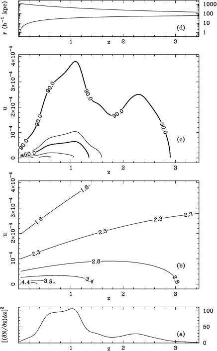
In order to understand the relative importance of the different factors in the integral, we separate them out in Fig. 1. The redshift distribution chosen for this illustration is [Sawicki et al.]’s (1997) photometric redshift distribution for the HDF galaxies (see also [Lanzetta et al.] 1996) in the three Wide Field Camera images of the Version 2 (1996 February 29) drizzled version of the data to $I_{AB,8140}<27$. The square of this distribution is shown in Fig. 1(a).

The redshift and distance dependence of $\xi[r(z,u),z]$ can be seen in Fig. 1(b). At any given $z,$ $\xi$ decreases as $u$ increases, since the spatial correlation decreases for increasing $r$, quickly approaching zero. Both the use of a fixed angle $\theta$ (chosen here as $\theta=4\hbox{${}^{\prime\prime}$}$, since the range of significant signal in [Villumsen et al.]’s $w_{0}$ HDF estimate is roughly $2{\cdot}5\hbox{${}^{\prime\prime}$}$ to $10\hbox{${}^{\prime\prime}$}$) and the choice of “stable clustering in proper coordinates” (i.e., $\epsilon=0$) contribute to the decrease in $\xi$ along the path for which $u\equiv 0.$ For large (fixed) $u,$ $r(z,u)$ becomes dominated by a nearly radial distance separation. Since $d^{2}d_{\mbox{\rm\small prop}}/dz^{2}<0,$ these separations become smaller for increasing $z,$ which would imply higher $\xi$ for clustering fixed in comoving coordinates ($\epsilon=\gamma-3$) as $z$ increases. Indeed, Fig. 1(b) shows that for “large” constant values of $u,$ the increase in $\xi$ as $z$ increases is strong enough to overcome the weakening of the amplitude of $\xi$ for higher $z.$

Fig. 1(c) shows that neither one nor the other of these limits in $u$ is sufficient to cover the domain in $z-u$ space which is relevant for the total value of the double integral. The maximum values of $u$ necessary to cover 90% of the numerator in Eq. 2 are less than about $0{\cdot}05\%$ of a redshift “unit”, but this is still large enough that the dominance of radial separation over perpendicular separation causes $\xi$ to increase as $z$ increases at a fixed $u,$ at least for $\theta=4\hbox{${}^{\prime\prime}$}.$

The smallness of the value of $u$ required to account for even 50% of the numerator of Eq. 2 is the key element required to interpret observational estimates of $w(\theta,m).$ In Fig. 1(d), the $u$ range covered in the $z-u$ plane plots is shown in units of (comoving) $h^{-1}$ kpc. Nearly all of the 90% contour is for galaxies separated by less than $1h^{-1}$ Mpc; much of the integral comes from separations less than $100h^{-1}$ kpc. This is the scale on which galaxy interactions and the relationship between galaxy haloes dominated by dark matter and the visible galaxies containing stars are likely to be complicated.

Other points to be noted in Fig. 1(c) are:

(1) [Sawicki et al.]’s (1997) redshift distribution includes many galaxies in the lowest redshift bins. Whether this is due to a genuinely steep faint end of the galaxy luminosity function or to the use of photometric rather than spectroscopic redshifts, it is not of cosmological interest to include spatial correlations of local dwarf galaxies within a few hundred kiloparsecs of the observer in estimates of $w($$z_{\mbox{\rm\small med}}$$)\,\lower 2.58334pt\hbox{$\buildrel>\over{\sim}$}\,1.$ It is therefore of importance to observe that the percentile contours concentrate towards lower and lower $z$ for higher values of the integrand (lower percentiles). The combination of rapidly decreasing separations, increasing values of $\xi(r,z)$ and slowness of $N_{z}(z,m)$ to decrease imply that a significant fraction of the signal in $w(\theta,m)$ could be due to very local galaxies.

For calculations presented below, a (conservative) lower limit is therefore set such that redshifts for which the perpendicular separation $r(z,0)$ is less than $10h^{-1}$ kpc are excluded from the domain of integration.

(2) [Sawicki et al.]’s (1997) $N_{z}$ peak at $z\approx 2{\cdot}3$ contributes significantly between the $70\%$ and $90\%$ contours, i.e., roughly $10\%$ of the numerator in Eq. 2 is due to this peak. Given the uncertainties in [Villumsen et al.]’s (1996) estimate of the HDF angular correlation function (essentially Poisson due to the small numbers of objects), this is not likely to be important for interpretation of the HDF data. However, for the brighter and more precise angular correlation function estimates (e.g., [Brainerd et al.] 1995) this could be more important—analytical single-peaked redshift distributions may not be precise enough.

Fig. 2.—: (a) (top panel) Dependence of $r_{\mbox{\rm\small eff}}^{p}$ [the median (comoving) radius which contributes a fraction $p$ of the double integral determining $w(\theta,m)$] on the growth rate $\epsilon$ of the spatial correlation function. The upper (lower) six curves are for $p=90\%;$ ($p=50\%$). Curves are thick for [Sawicki et al.]’s (1997) HDF $I_{AB,8140}<27$ photometric redshift distribution and thin for the analytical distribution of Eq. 3 with $z_{0}=1{\cdot}20$ (having the same $z_{\mbox{\rm\small med}}$ as [Sawicki et al.]’s redshift distribution). Different cosmological models are shown [in (a)-(c)] by solid ($\Omega_{0}=1,\lambda_{0}=0$), dotted ($\Omega_{0}=0{\cdot}1,\lambda_{0}=0$) and dashed ($\Omega_{0}=0{\cdot}1,\lambda_{0}=0{\cdot}9$) curves. (b) (middle panel) Dependence of $r_{\mbox{\rm\small eff}}^{p}$ on $z_{0},$ adopting Eq. 3 (for which $z_{0}\approx 0{\cdot}95$ $z_{\mbox{\rm\small med}}$), shown divided by minimum perpendicular distance at a given redshift $r_{\perp}\equiv r(z_{0},0).$ Upper (lower) three curves are for $p=90\%;$ ($p=50\%$). (c) (bottom panel) Dependence of $r_{\perp}\equiv r(z_{0},0)$ on $z_{0}$ (equivalent to the angular diameter-redshift relation). Parameter values held constant in all curves are $\theta=4$^′′, $r_{0}=5{\cdot}5h^{-1}$ Mpc and $\gamma=1{\cdot}8.$

3 THE EFFECTIVE SEPARATION $r_{\mbox{\rm\small eff}}^{p}$

Of course, the values of the separation scales which contribute most of the value of $w(\theta,m)$ discussed above are for a particular choice of the parameters chosen in Eq. 1 (or on the validity of this equation at such scales), the redshift distribution, $\theta$ and the cosmological model. In order to discuss dependence of the separation scales on Eq. 1, on the $z_{\mbox{\rm\small med}}$ and the shape of the redshift distribution, on $\theta$ and on cosmological parameters, it is useful to define the effective separation, $r_{\mbox{\rm\small eff}}^{p}$, to be the median value of $r(z,u)$ over the domain in $z-u$ space inside a contour of constant $N_{z}^{2}(z,m)\xi[r(z,u),z]$ which contributes a fraction $p$ of the value of $w(\theta,m)$ (where the denominator in Eq. 2 is held fixed).

3.1 Dependence on the Spatial Correlation Function

Lowering the value of $r_{0}$ (which is considered by, e.g., [Bernstein et al.] 1994; [Brainerd et al.] 1995, to denote a possible transition in galaxy “populations”) factors out of Eq. 2 as a constant; it reduces the value of $w$ but does not affect the question of which separations are relevant to the integral. Reducing the value of $\gamma$ (for fixed $\epsilon-\gamma$ in order not to affect the redshift evolution of $\xi$) would increase the values of $r_{\mbox{\rm\small eff}}^{p}$ slightly. In estimates of $w$ for faint galaxies, it is usually assumed that $\gamma-1=0{\cdot}8$ in order to correct for the integral constraint, so this is the value of interest here (e.g., [Hudon & Lilly] 1996; though note [Campos et al.] 1995; [Infante & Pritchet] 1995).

Of more interest is the value of $\epsilon,$ which as mentioned above has either theoretically or observationally motivated values lying in the range from $-1{\cdot}2$ to nearly $3.$

Fig. 2(a) shows that in spite of the wide range in values of $\epsilon,$ the dependence of $r_{\mbox{\rm\small eff}}^{p}$ on $\epsilon$ is weak. Even for a cosmological constant dominated flat cosmological model and $\epsilon=3,$ $r_{\mbox{\rm\small eff}}^{p}$ for [Sawicki et al.]’s (1997) redshift distribution is no more than a factor of two lower than that for the analytical distribution.

Although weak, there is an average trend to lower values for higher $\epsilon.$ Higher $\epsilon$ means a more rapid decrease in spatial correlation amplitude with $z,$ so that the correlations at lower $z$ contribute relatively more to the integral. The lower the value of $z,$ the lower the (comoving) perpendicular separations $r(z,0),$ for any cosmological model. Hence, the slight decrease in $r_{\mbox{\rm\small eff}}^{p}$.

In other words, independently of the growth rate of the spatial correlation function, angular correlations in deep surveys of faint galaxies only probe length scales characteristic of galactic haloes.

The stronger decrease in $r_{\mbox{\rm\small eff}}^{p}$ for the observational (photometric) redshift distribution than for the analytical distribution of the same $z_{\mbox{\rm\small med}}$ can be attributed to its complex shape. Once $\epsilon$ has increased enough that the $z\approx 2{\cdot}2$ peak no longer contributes much, the effective $z_{\mbox{\rm\small med}}$ of the observational distribution will be lower than that of the analytical distribution; thus, the lower $r_{\mbox{\rm\small eff}}^{p}$ values.

The trend to lower $r_{\mbox{\rm\small eff}}^{p}$ is not monotonic for the observational redshift distribution. This is attributable to an increase in the relative importance of $u$ separations to perpendicular separations when $N_{z}^{2}(z,m)(1+z)^{-(3+\epsilon-\gamma)}$ becomes flatter. A “complex” enough redshift distribution could possibly increase the importance of this reversed dependence of $r_{\mbox{\rm\small eff}}^{p}$ on $\epsilon,$ as indeed is seen below.

3.2 Dependence on the Redshift Distribution

Fig. 3.—: The dependence of $r_{\mbox{\rm\small eff}}^{p}$ on the shape of $N_{z}$ is shown by reproducing Fig. 2(a), but replacing the $N_{z}$ estimate of [Sawicki et al.] (1997) by those of (a) [Lanzetta et al.] (1996), (b) [Mobasher et al.] (1996, Fig.2) and (c) [Gwyn & Hartwick] (1996), and using analytical distributions with appropriate $z_{0}$ values (a) $z_{0}=1{\cdot}15$, (b) $z_{0}=1{\cdot}6$ and (c) $z_{0}=2{\cdot}0.$ Axes and line styles are as for Fig. 2(a).

Fig. 4.—: The shapes of the photometric redshift distributions $N_{z}$ estimated by [Sawicki et al.] (1997), [Lanzetta et al.] (1996), [Mobasher et al.] (1996) and [Gwyn & Hartwick] (1996) for the HDF are shown here against redshift, normalised for purposes of comparison. The dependence of $r_{\mbox{\rm\small eff}}^{p}$ on the different shapes is shown in Figs 2(a), 3(a), 3(b), 3(c) as indicated.

The effective separation $r_{\mbox{\rm\small eff}}^{p}$ depends on a redshift distribution primarily via the typical redshifts in the sample, or more quantitatively, on the median redshift, $z_{\mbox{\rm\small med}}$, of $N_{z}.$ This dependence is analysed here by use of the simple analytical distribution

$$z^{2}\exp[-(z/z_{0})^{\beta}],$$ (3)

where $\beta=2{\cdot}5$ (as in [Efstathiou et al.] 1991; [Villumsen et al.] 1996). For this distribution, $z_{\mbox{\rm\small med}}$ dependence translates directly into dependence on $z_{0},$ since $z_{\mbox{\rm\small med}}$ $\approx 0.95z_{0}$.

A very useful property of this dependence is shown in Fig. 2(b): nearly all of this $z_{0}$ dependence is in the (equivalent of the) angular diameter-redshift relation, shown as the dependence of the perpendicular separation $r_{\perp}(z)\equiv r(z,u=0)$ on $z$ in Fig. 2(c).

Both $r_{\mbox{\rm\small eff}}^{50\%}$ and $r_{\mbox{\rm\small eff}}^{90\%}$ are nearly constant over a wide range in $z_{0}.$ Moreover, $r_{\mbox{\rm\small eff}}^{50\%}$ is only about $5\%-15\%$ greater than $r_{\perp}(z_{0}),$ i.e., about $10\%-20\%$ greater than $r_{\perp}($$z_{\mbox{\rm\small med}}$$).$ Relative to the precision of present cosmological measurements, it can be said that $r_{\perp}($$z_{\mbox{\rm\small med}}$$)$ is a very good estimator for $r_{\mbox{\rm\small eff}}^{50\%}$ for such analytical distributions. In addition, since $r_{\mbox{\rm\small eff}}^{50\%}$ is insensitive to $\epsilon$ and since the $\epsilon$ dependence of both the observational (photometric) and analytical $N_{z}$ curves are similar (Fig. 2), the quality of $r_{\perp}($$z_{\mbox{\rm\small med}}$$)$ as an estimator for $r_{\mbox{\rm\small eff}}^{50\%}$ is little dependent on the value of $\epsilon$ and the precise shape of $N_{z},$ avoiding the need for explicit integration of Limber’s Equation (Eq. 2).

The $90\%$ percentile median separation $r_{\mbox{\rm\small eff}}^{90\%}$ is about $4-4{\cdot}5$ times $r_{\perp}(z_{0}),$ depending on $z_{0}$ and cosmological model to no more than about $10\%.$ Again, the relative robustness of $r_{\mbox{\rm\small eff}}^{p}$ to $\epsilon$ implies that a constant value of $r_{\mbox{\rm\small eff}}^{90\%}$ in this range can be used for practical purposes without integration of Limber’s Equation being required.

The dependence of $r_{\mbox{\rm\small eff}}^{p}$ on the shape of $N_{z}$ is not totally negligible. This can be seen to some extent in Fig. 2(a), which shows that for the same $z_{\mbox{\rm\small med}}$, the values of $r_{\mbox{\rm\small eff}}^{p}$ can differ by up to about a factor of two.

To confirm this more explicitly, various published photometric redshift distributions estimated for the HDF have been adopted in place of that of [Sawicki et al.] (1997) and the resulting dependence of $r_{\mbox{\rm\small eff}}^{p}$ on $\epsilon$ for these $N_{z}$ estimates are presented in Fig. 3. The $N_{z}$ estimates adopted are shown in Fig. 4.

The results are similar to those for [Sawicki et al.]’s (1997) $N_{z},$ though the maximum difference between photometric and analytical distributions increases from about a factor of two to a factor of three to four for $r_{\mbox{\rm\small eff}}^{90\%}$ in the case of high $\epsilon$ values. The bimodality of [Gwyn & Hartwick]’s (1996) $N_{z}$ and the high resolution of [Mobasher et al.]’s (1996) $N_{z}$ make this hardly very surprising.

The large differences between the photometric and analytical distributions for [Gwyn & Hartwick]’s (1996) $N_{z}$ are mainly due to the low $z$ peak. Obviously there is uncertainty in the correctness of photometric redshifts, but if $N_{z}$ (HDF) really was as bimodal as [Gwyn & Hartwick] (1996) estimated with a strong low $z$ peak, then not only would many galaxy pairs which contribute to $w_{0}$ be closer to one another than would be expected from an analytical unimodal distribution, but a large part of the $w_{0}$ signal would be from non-cosmological distances, at which $r_{\perp}\sim 10h^{-1}$ kpc. In this case, the meaning of a $w_{0}$ estimate would have to be analysed in considerable detail, or else redshift separation would have to be used to estimate $w(r_{p})$ ([Davis & Peebles] 1983) rather than $w_{0}$ in order to extract quantities with simple physical meaning.

In summary, the earlier photometric redshift distributions to that deduced by [Sawicki et al.] (1997) imply similar values of $r_{\mbox{\rm\small eff}}^{p}$ to those of [Sawicki et al.] to within much less than an order of magnitude.

It should also be noted that changing the limiting magnitude of the survey or changing the value of $\beta$ is equivalent to a change in $z_{\mbox{\rm\small med}}$ and/or in the shape of $N_{z}.$

3.3 Dependence on Other Parameters

Since $r(z,u)$ is dominated by the perpendicular separation $r(z,u=0)=\theta\,d_{\mbox{\rm\small prop}}(z)$ (for $\theta\ll 1$ rad), $r_{\mbox{\rm\small eff}}^{p}$ is nearly proportional to $\theta.$ Indeed, although the line-of-sight galaxy separation for a given $z$ is not directly proportional to $\theta$ [i.e., $r(z,u,\theta_{2})/r(z,u,\theta_{1})\neq\theta_{2}/\theta_{1}$ if $u\neq 0$], the required domain in $u$ to obtain a fraction $p$ of the integral of $w(\theta,m)$ expands sufficiently (but remains small enough) that the value of $r_{\mbox{\rm\small eff}}^{p}$ remains proportional to $\theta$ to the precision of the calculation (for $p=50\%$ and $p=90\%$).

Values of $r_{\mbox{\rm\small eff}}^{50\%}$ and $r_{\mbox{\rm\small eff}}^{90\%}$ for the nominal angle of [Villumsen et al.]’s (1996) $w$ determination [$w(\theta,m)$ is normally interpolated or extrapolated to the same angle for a large number of different surveys in order to compare the relative amplitudes of the surveys], i.e., $\theta=$ 1^′′, imply $r_{\mbox{\rm\small eff}}^{p}$ values four times lower than those displayed in Fig. 2, i.e., $r_{\mbox{\rm\small eff}}^{50\%}$ $\sim 10h^{-1}$ kpc and $r_{\mbox{\rm\small eff}}^{90\%}$ $\sim 40h^{-1}$ kpc. While such a nominal angle is primarily meant for comparison of amplitudes of $w,$ the physical meaningfulness or otherwise should obviously be kept in mind when examining such figures!

Brighter faint galaxy surveys having most of their signal at, say, 40^′′, would have their $r_{\mbox{\rm\small eff}}^{p}$ values multiplied by ten, i.e., $r_{\mbox{\rm\small eff}}^{50\%}$ $\sim 500h^{-1}$ kpc and $r_{\mbox{\rm\small eff}}^{90\%}$ $\sim 1500h^{-1}$ kpc.

The effects of cosmological parameters on $r_{\mbox{\rm\small eff}}^{p}$ are shown in panels (a) and (c) of Fig. 2: since $dd_{\mbox{\rm\small prop}}/dz$ is successively larger for hyperbolic and cosmological constant dominated, flat cosmologies, the values of $r(z_{0},0)$ and consequently $r_{\mbox{\rm\small eff}}^{p}$ increase respectively. The increase in $r(z_{0},0)$ is in fact faster than that of $r_{\mbox{\rm\small eff}}^{p}$, so that Fig. 2(b) shows a slight reversal in this dependence for the ratio $r_{\mbox{\rm\small eff}}^{p}$$/r(z_{0},0),$ though the main effect is in $r(z_{0},0).$

4 DISCUSSION

The results above can be summarised as order of magnitude estimates:

$$r_{\mbox{\rm\small eff}}^{p} = (1+\Delta_{p})\;r_{\perp}[\mbox{$z_{\mbox{\rm\small med}}$}(N_{z})]$$ (4)

where

$$r_{\perp}[\mbox{$z_{\mbox{\rm\small med}}$}(N_{z})] \equiv r[z=\mbox{$z_{\mbox{\rm\small med}}$}(N_{z}),u=0,\Omega_{0}=1,$$

$$\lambda_{0}=0]$$

$$= \theta\,d_{\mbox{\rm\small prop}}[\mbox{$z_{\mbox{\rm\small med}}$}(N_{z}),\Omega_{0}=1,\lambda_{0}=0]$$

$$= {2c\over H_{0}}\,\theta\left(1-{1\over\sqrt{1+\mbox{$z_{\mbox{\rm\small med}}$}(N_{z})}}\right)$$

and

$$1\,\lower 2.58334pt\hbox{$\buildrel<\over{\sim}$}\,\Delta_{50}\,\lower 2.58334pt\hbox{$\buildrel<\over{\sim}$}\,2$$

$$2\,\lower 2.58334pt\hbox{$\buildrel<\over{\sim}$}\,\Delta_{90}\,\lower 2.58334pt\hbox{$\buildrel<\over{\sim}$}\,7$$ (6)

for $\gamma=-1{\cdot}8,$ $-1{\cdot}2<\epsilon<3,$ $0{\cdot}1<\Omega_{0}<1{\cdot}0,$ $0{\cdot}0<\lambda_{0}<1-\Omega_{0},$ $1<\mbox{$z_{\mbox{\rm\small med}}$}(N_{z})<2{\cdot}5$ and for $N_{z}$ shapes as “smooth” as in Eq. 3 or no “rougher” than that of [Sawicki et al.]’s (1997) redshift distribution.

These relations enable $r_{\mbox{\rm\small eff}}^{p}$ to be estimated for observational angular correlation function measurements. Many of the brighter ($B\,\lower 2.58334pt\hbox{$\buildrel<\over{\sim}$}\,24,$ $V\,\lower 2.58334pt\hbox{$\buildrel<\over{\sim}$}\,25$ or $R\,\lower 2.58334pt\hbox{$\buildrel<\over{\sim}$}\,26$) faint galaxy angular correlation measurements ([Neuschaefer et al.] 1991; [Pritchet & Infante] 1992; [Couch et al.] 1993; [Infante & Pritchet] 1995) show significant power law correlations on scales ranging from $\sim 10\hbox{${}^{\prime\prime}$}$ to $\sim 10\hbox{${}^{\prime}$}.$ Adopting $z_{\mbox{\rm\small med}}$ $\approx 0{\cdot}5$ as a typical value for the above surveys, which should give $r_{\perp}$ to be correct within better than an order of magnitude, Eqs 4-6 (which remain valid under extrapolation to $z_{\mbox{\rm\small med}}$ $=0{\cdot}5$) imply that $50h^{-1}$ kpc  $\buildrel<\over{\sim}$  $r_{\mbox{\rm\small eff}}^{50\%}$ $\,\lower 2.58334pt\hbox{$\buildrel<\over{\sim}$}\,3h^{-1}$ Mpc and $200h^{-1}$ kpc  $\buildrel<\over{\sim}$  $r_{\mbox{\rm\small eff}}^{90\%}$ $\,\lower 2.58334pt\hbox{$\buildrel<\over{\sim}$}\,12h^{-1}$ Mpc for these angular ranges. Spatial correlations are well established at most of these spatial separations, so interpretation in terms of Eq. 1 is likely to be a good first approximation.

Possibly of interest in these cases is the higher end of the length scales. [Loveday et al.] (1992) only consider their power law fit to $\xi(r)$ to be good to about $20h^{-1}$ kpc. The surveys covering the largest solid angles may well be affected by—or be used to estimate—spatial correlations at separations difficult to measure by local surveys such as the Stromlo-APM survey of [Loveday et al.] Indeed, [Infante & Pritchet] (1995) discuss the degree to which their data is affected by the large scale behaviour of $\xi(r).$ Their angular correlation functions extend to about $0{\cdot}4^{\circ}.$ The analysis here implies that at $0{\cdot}4^{\circ},$ $r_{\mbox{\rm\small eff}}^{90\%}$ $\sim 30h^{-1}$ Mpc, so careful analysis of this data might be able to produce estimates of the perturbation power spectrum on scales comparable to that in the Stromlo-APM survey.

The brighter angular correlation measurements on smaller fields (e.g., [Efstathiou et al.] 1991; [Roukema & Peterson] 1994; [Brainerd et al.] 1995) cover smaller angular ranges, from $\sim 10\hbox{${}^{\prime\prime}$}$ to $\sim 1\hbox{${}^{\prime}$},$ so again adopting $z_{\mbox{\rm\small med}}$ $\approx 0{\cdot}5$ implies that $50h^{-1}$ kpc  $\buildrel<\over{\sim}$  $r_{\mbox{\rm\small eff}}^{50\%}$ $<$ $r_{\mbox{\rm\small eff}}^{90\%}$ $\,\lower 2.58334pt\hbox{$\buildrel<\over{\sim}$}\,1.2h^{-1}$ Mpc for these observations. This is again within typical estimates of power law behaviour for $\xi(r),$ e.g., [Davis & Peebles] (1983) and [Loveday et al.] (1992), though $50h^{-1}$ kpc is already smaller than typical estimates of the radii of the haloes of $L^{*}$ (bright) galaxies.

Raising the estimate of $z_{\mbox{\rm\small med}}$ from 0.5 to $z_{\mbox{\rm\small med}}$ $=1{\cdot}2$ (the value for [Sawicki et al.]’s HDF analysis) would double each of these separation sizes. Alternatively, conversion to proper units, which are relevant if considering galaxy haloes at $z\approx 1$ to be collapsed and dynamically stable objects, requires division by $(1+z)\approx 2,$ i.e., halving the separation estimates.

This brings us back to the worry raised above—that spatial correlations are being measured for galaxies which are closer together than the radii of their parent haloes! However, since a large part of the signal in the cases just-mentioned comes from larger separations, this should not affect the observational validity of using Eq. 1 as a first order estimator.

The reliance upon small separations becomes a stronger concern for the angular correlation function of the HDF galaxies (and for possible future estimates of $w(\theta,m)$ using the HST, the Next Generation Space Telescope, or if adaptive optics can be used for faint fields using ground-based telescopes).

The $I_{AB}<27$ limit of [Sawicki et al.]’s (1996) analysis of the HDF galaxies corresponds to $I\,\lower 2.58334pt\hbox{$\buildrel<\over{\sim}$}\,26{\cdot}5$ (in the standard Vega-based system), and the range of the galaxies’ colours (e.g., [Metcalfe et al.] 1996) is approximately $0\,\lower 2.58334pt\hbox{$\buildrel<\over{\sim}$}\,R-I\,\lower 2.58334pt\hbox{$\buildrel<\over{\sim}$}\,2.$ Hence, the redshifts appropriate for [Villumsen et al.]’s (1996) $R$-band magnitude ranges $R<26{\cdot}5$ to $R<28{\cdot}5$ used in estimating $w(\theta,m)$ should be similar to those in [Sawicki et al.]’s analysis, though the bluest galaxies not present in [Sawicki et al.]’s (1997) analysis could be expected to be at somewhat lower redshifts. If we consider the range of significant signal in [Villumsen et al.]’s (1996) estimate to be from $2{\cdot}5\hbox{${}^{\prime\prime}$}$ to $10\hbox{${}^{\prime\prime}$},$ this then implies for $z_{\mbox{\rm\small med}}$ $\approx 1{\cdot}2$ that $25h^{-1}$ kpc  $\buildrel<\over{\sim}$  $r_{\mbox{\rm\small eff}}^{50\%}$ $<$ $r_{\mbox{\rm\small eff}}^{90\%}$ $\,\lower 2.58334pt\hbox{$\buildrel<\over{\sim}$}\,400h^{-1}$ kpc for these observations.

In this case, almost none of the signal comes from separations for which [Loveday et al.] (1992) found significant correlations fit by a power law, and the similarity to halo sizes is significant. Possibly one of the neatest measurements of halo extent is by Lyman-$\alpha$ and metal line absorption systems in front of quasars. For instance, [Bergeron & Boissé] (1991), [Bechtold et al.] (1994), [Lanzetta et al.] (1995), [Fang et al.] (1996) and [Le Brun et al.] (1996) estimate gaseous halo radii for both sorts of systems of around $50-200h^{-1}$ kpc. This range matches very closely the range in $r_{\mbox{\rm\small eff}}^{p}$ just mentioned.

[However, it should be noted that (1) the Lyman-$\alpha$ systems may not be associated with galaxies (e.g., [Le Brun et al.] 1996) and (2) there is marginal rotation curve evidence that the halo of the Galaxy is no more than 15 kpc in radius ([Honma & Sofue] 1996, but see [Binney & Dehnen] 1997), implying a mass for the Galaxy about an order of magnitude smaller than most estimates.]

Is the value of $z_{\mbox{\rm\small med}}$ adopted here too low? While [Sawicki et al.]’s (1997) photometric redshift analysis uses template spectra which account for both internal reddening and high-$z$ Lyman absorption, earlier analyses, e.g., [Mobasher et al.] (1996), suggested that $z_{\mbox{\rm\small med}}$ should be as high as $z_{\mbox{\rm\small med}}$ $=2{\cdot}1.$ Even if the redshifts of the $R$-selected sample contributing to [Villumsen et al.]’s $w(\theta,m)$ estimates (or to independent estimates of, say, an $I$-selected sample) were as high as $z_{0}\approx 2{\cdot}1,$ these effective separations would only increase by about $30\%-50\%$ (depending on cosmology), according to Eqs 4-6. The spatial separations would still correspond to typical estimates of galaxy halo radii, particularly when applying the conversion from comoving to proper coordinates. Note that the values adopted for use in Eq. 3 in [Villumsen et al.]’s (1996) models shown in their Fig. 2 for $R<26{\cdot}5$ to $R<28{\cdot}5$ are $1{\cdot}4\,\lower 2.58334pt\hbox{$\buildrel<\over{\sim}$}\,z_{0}\,\lower 2.58334pt\hbox{$\buildrel<\over{\sim}$}\,1{\cdot}8.$

Table 1:: Values of $r_{\mbox{\rm\small eff}}^{p}$ for $1\hbox{${}^{\prime\prime}$}$ for redshifts $z=2{\cdot}5$ and $z=5$ spanning redshifts likely for the HDF objects colour-selected to high redshift by [Colley et al.] (1996; 1997), assuming that Eqs 4-6 can be validly extrapolated to these objects. These effective separations are in units of $h^{-1}$ kpc, comoving or proper as indicated.

$p$	cosm.		comoving		proper
	$\Omega_{0}$	$\lambda_{0}$	$z=2{\cdot}5$	$z=5$	$z=2{\cdot}5$	$z=5$
50%	$1{\cdot}0$	$0{\cdot}0$	14	17	4	3
50%	$0{\cdot}1$	$0{\cdot}0$	21	35	6	6
50%	$0{\cdot}1$	$0{\cdot}9$	26	37	7	6
90%	$1{\cdot}0$	$0{\cdot}0$	54	69	16	12
90%	$0{\cdot}1$	$0{\cdot}0$	86	141	24	24
90%	$0{\cdot}1$	$0{\cdot}9$	103	147	30	25

This result brings to mind the suggestions, based on morphological analysis of the HST Medium Deep Survey (MDS) and the HDF ([Griffiths et al.] 1994; [Casertano et al.] 1995; [Driver et al.] 1995a,b; [Glazebrook et al.] 1995; [Abraham et al.] 1996; [van den Bergh et al.] 1996), that many of the HDF galaxies are the “building blocks” of future galaxies which later merge together. ([Pascarelle et al.] (1996) make a similar suggestion based on HST imaging and Multiple Mirror Telescope spectroscopic redshifts.) In this case, the HDF galaxies’ haloes should be smaller than present day galaxy haloes, and so the visible galaxies could be correlated without their haloes necessarily overlapping.

However, [Davis & Peebles]’s (1983) observation of correlated galaxies down to $10h^{-1}$ kpc is a local observation, it is not an observation of primordial galaxies. It is quite noisy, so perhaps is already affected by the detailed nature of the galaxy-halo relationship. In either case, the angular correlation function of the HDF must be affected by, and hence offer some clues to, the relationship between galaxies and haloes.

A complementary analysis to that presented here is that of [Colley et al.] (1996; 1997). [Colley et al.] (1996) measured a very strong angular correlation for “galaxies” selected by colour to be at high redshifts ($z\,\lower 2.58334pt\hbox{$\buildrel>\over{\sim}$}\,2$) and point out that the detected objects may in fact be star-forming regions within “normal” galaxies, dimmed only by $(1+z)^{2}$ in surface brightness rather than $(1+z)^{4}$ since they are (nearly) unresolved by the HST. In [Colley et al.] (1997), apart from a dynamical discussion of different scenarios, the authors add a nearest-neighbour analysis which strengthens their argument that there is an excess of close objects separated by less than about $1\hbox{${}^{\prime\prime}$}.$

The result of the effective separation calculations presented here only strengthens [Colley et al.]’s model. As they point out in their conclusions ([Colley et al.] 1997), two galaxies at identical redshifts separated by $1\hbox{${}^{\prime\prime}$}$ at the redshift range of their sample are separated by roughly 6 kpc in proper units. Since $r_{\mbox{\rm\small eff}}^{p}$ $\sim r_{\perp},$ if the objects were indeed individual galaxies, and if a much larger field were measured in order to reliably measure $w(\theta,m)$ at these small angles and faint magnitudes, then about 50% of the spatial correlation signal would be from galaxies separated by less than about $6h^{-1}$ kpc, and 90% of the signal for galaxies closer to one another than about $24h^{-1}$ kpc. These values, in both comoving and proper coordinates in order to facilitate deductions from both cosmological and galaxy formation points of view, are presented in Table 1.

Returning to the full sample of the HDF galaxies, for which $25h^{-1}$ kpc  $\buildrel<\over{\sim}$  $r_{\mbox{\rm\small eff}}^{50\%}$ $<$ $r_{\mbox{\rm\small eff}}^{90\%}$ $\,\lower 2.58334pt\hbox{$\buildrel<\over{\sim}$}\,400h^{-1}$ kpc, are there any justified alternatives to the extension of Eq. 1 to these separations, either observationally or theoretically?

A comparison of the theoretical evolution of the spatial correlation function to [Villumsen et al.]’s (1996) HDF estimates is given by [Matarrese et al.] (1996), for an $\Omega_{0}=1,\lambda_{0}=0$ CDM universe where the full linear and non-linear evolution is given by a formula fit to gravity-only N-body simulations ([Hamilton et al.] 1991; [Jain et al.] 1995). [Matarrese et al.]’s (1996) Fig. 5 (for no bias factor) is approximately consistent with the HDF correlations, whilst [Villumsen et al.] (1996) found that a spatial correlation growth rate of $\epsilon=0{\cdot}8$ in Eq. 1 was not sufficient to provide low enough correlations unless the value of $r_{0}$ is decreased, i.e., that a transition in populations is hypothesised. Differences at the sub-Mpc level could explain this better fit. However, the CDM simulations used for [Jain et al.]’s formula have only 1 particle/(350$h^{-1}$ kpc)³ and a force resolution of 32 $h^{-1}$ kpc, so may not be valid at these scales. Additionally, of course, they cannot address the question of how to relate stellar galaxies to dark matter dominated haloes—unless this is governed by gravity alone, which seems unlikely.

An empirical, but theoretically motivated, alternative would be [Peacock]’s (1996) analysis based on a two-power law fit to galaxy correlations of the APM ([Maddox et al.] 1990a; 1990b) and IRAS ([Saunders et al.] 1992) surveys. However, [Peacock] finds that this fit implies that for an $\Omega_{0}=1,\lambda_{0}=0$ universe, an extra correlation at scales of $r\,\lower 2.58334pt\hbox{$\buildrel<\over{\sim}$}\,2\pi h^{-1}$ Mpc is needed to fit the CFRS ([CFRS-VIII] 1996) data, unless a scale-dependent bias factor is used in combination with a constant bias factor. [Matarrese et al.]’s (1996) use of [Jain et al.]’s (1995) N-body motivated $\xi(r,z)$ description better fits the CFRS data (for no bias), so would maybe more appropriate for an extension of the present work.

An alternative empirical improvement to Eq. 1 could be to use the $w$ estimates of [Infante et al.] (1996) on very small scales (down to $\approx 1\hbox{${}^{\prime\prime}$}$) in a survey covering a very large solid angle ($2{\cdot}3$ sq.deg.), hence, having enough precision to make such estimates. [Infante et al.] (1996) find that at the smallest separations, $2\hbox{${}^{\prime\prime}$}\,\lower 2.58334pt\hbox{$\buildrel<\over{\sim}$}\,\theta\,\lower 2.58334pt\hbox{$\buildrel<\over{\sim}$}\,6\hbox{${}^{\prime\prime}$}$, there is a correlation signal about a factor of three higher than that of a $\gamma=1{\cdot}8$ power law extrapolated from larger angles. To the extent that the above $r_{\mbox{\rm\small eff}}^{p}$ calculations can be extrapolated to this “highly non-linear” case, the value $r_{\perp}=24h^{-1}$ kpc (as defined in Eq. LABEL:e-reffrp) implies that half of this signal comes from three-dimensional galaxy pair separations of about this size, and 40% more comes from separations up to about $100-200h^{-1}$ kpc. (Note that [Infante et al.] adopt proper units. The conversion follows from using $z_{\mbox{\rm\small med}}$ $=0{\cdot}35.$) The values of $\xi(r,z)$ for $r\,\lower 2.58334pt\hbox{$\buildrel<\over{\sim}$}\,20h^{-1}$ kpc, without contamination from “normal” correlations at larger angles, could therefore be even higher than might be expected from simple inspection of [Infante et al.]’s (1996) figures.

5 CONCLUSIONS

In order to see what length scales and redshifts correspond to the spatial correlations $\xi(r,z)$ represented in recent measurements of the faint galaxy angular correlation function $w(\theta,m),$ Limber’s Equation (Eq. 2) has been examined over a range of likely possibilities for $\xi$ and $N_{z}(z,m).$ The separation into $N_{z}(z,m)$ and $\xi[r(z,u),z]$ and the contours in the $z-u$ plane which contribute to the integral have been shown, revealing that observational $w$ measurements combine spatial correlations from a wide range in mean redshift.

A simple definition of an effective separation $r_{\mbox{\rm\small eff}}^{p}$ to quantify the relevant length scales for $w$ has been defined as the median (comoving) separation within the contour of constant $(\partial N/\partial z)^{2}\xi[r(z,u),z]$ contributing a fraction $p$ of the numerator of Eq. 2. This is similar in order of magnitude to the perpendicular distance $r_{\perp}\equiv d_{\mbox{\rm\small prop}}\theta$ at the characteristic redshift, $z_{0}$, of simple analytical redshift distributions (Eq. 3), and hence to the median redshifts of such distributions.

More precisely, for the parameter space covered, $r_{\mbox{\rm\small eff}}^{50\%}$ is about $5\%-15\%$ greater than $r_{\perp}(z_{0}),$ i.e., about $10\%-20\%$ greater than $r_{\perp}($$z_{\mbox{\rm\small med}}$$)$ (for $\beta=2{\cdot}5$ in Eq. 3); while $r_{\mbox{\rm\small eff}}^{90\%}$ is about $4-4{\cdot}5$ times $r_{\perp}(z_{0}).$

For a more realistic redshift distribution, e.g., the photometric redshift distribution of [Sawicki et al.] (1997), $r_{\mbox{\rm\small eff}}^{p}$ may be different by up to about a factor of two to the $r_{\mbox{\rm\small eff}}^{p}$ values for the analytical redshift distributions if $-1{\cdot}2<\epsilon<3.$

In summary, values of $r_{\mbox{\rm\small eff}}^{p}$ for typical median redshifts of most faint galaxy angular correlation measurements indicate that the use of Eq. 1 does not imply an extrapolation (in galaxy pair separation) much below or above observational spatial correlation measurements. (The validity of redshift dependence scaling by $(1+z)^{-(3+\epsilon-\gamma)}$ is not tested, however.)

The scales on which HDF galaxies are correlated (as measured by [Villumsen et al.] 1996) imply comoving separations of $25h^{-1}$ kpc  $\buildrel<\over{\sim}$  $r_{\mbox{\rm\small eff}}^{50\%}$ $<$ $r_{\mbox{\rm\small eff}}^{90\%}$ $\,\lower 2.58334pt\hbox{$\buildrel<\over{\sim}$}\,400h^{-1}$ kpc. That is, for typical redshifts over $z\,\lower 2.58334pt\hbox{$\buildrel>\over{\sim}$}\,1,$ a substantial fraction of the angular correlation signal is generated by galaxies spatially separated, in proper units, by around $10-100h^{-1}$ kpc. While spatial correlations of galaxies at these separations have been observed for local galaxies ([Davis & Peebles] 1983), this is a scale at which halo and/or galaxy existence, let alone interactions, might strongly modify the spatial correlation function.

We wish to dedicate this paper to the memory of the late Prof. Roger Tayler, whose support for this collaboration was well appreciated. We thank Alain Blanchard for useful discussion on this topic and B. Mobasher for providing tables in electronic format. BFR acknowledges a Centre of Excellence Visiting Fellowship (National Astronomical Observatory of Japan, Mitaka), support from PPARC and from Starlink computing resources.

References

- Abraham et al. Abraham, R.G., Tanvir, N.R., Santiago, B.X., Ellis, R.S., Glazebrook, K. & van den Bergh, S., 1996, MNRAS, 279, L47
- Bechtold et al. Bechtold, J., Crotts, A.P.S., Duncan, R.C. & Fang, Y.-H., 1994, ApJ, 437, 83L
- Bergeron & Boissé Bergeron, J. & Boissé, P., 1991, A&A, 243, 344
- Bernstein et al. Bernstein, G.M., Tyson, J.A., Brown, W.R. & Jarvis, J.F., 1994, ApJ, 426, 516
- Binney & Dehnen Binney, J. & Dehnen, W., 1997, MNRAS , 287, L5
- Brainerd et al. Brainerd, T.G., Smail, I. & Mould, J., 1995, MNRAS, 275, 781
- Campos et al. Campos, A., Yepes, G., Carlson, M., Klypin, A.A., Moles, M. & Joergensen, H., 1995, Clustering in the Universe (XXX Rencontres de Moriond), ed. S. Maurogodato et al., Gif-sur-Yvette: Editions Frontières, 403
- Casertano et al. Casertano, S., Ratnatunga, K.U., Griffiths, R.E., Im, M., Neuschaefer, L.W., Ostrander, E.J. & Windhorst, R.A., 1995, ApJ, 453, 599
- Cole et al. Cole, S., Ellis, R., Broadhurst, T. & Colless, M., 1994, MNRAS, 267, 541
- Colley et al. Colley, W.N., Rhoads, J.E., Ostriker, J.P. & Spergel, D.N., 1996, ApJ, 473, L63 (astro-ph/9603020)
- Colley et al. Colley, W.N., Gnedin, O.Y., Ostriker, J.P. & Rhoads, J.E., 1997, astro-ph/9702030
- Couch et al. Couch, W.J., Jurcevic, J.S. & Boyle B.J., 1993, MNRAS, 260, 241
- Davis & Peebles Davis, M. & Peebles, P.J.E., 1983, ApJ, 267, 465
- Driver et al. Driver, S.P., Windhorst, R.A. & Griffiths, R.E., 1995a, ApJ, 453, 48
- Driver et al. Driver, S.P., Windhorst, R.A., Ostrander, E.J., Keel, W.C., Griffiths, R.E. & Ratnatunga, K.U., 1995b, ApJ, 449, L23
- Efstathiou et al. Efstathiou, G., Bernstein, G., Katz, N., Tyson, J. A. & Guhathakurta, P., 1991, ApJ, 380, L47
- Fang et al. Fang, Y.-H., Duncan, R.C., Crotts, A.P.S. & Bechtold, J., 1996, ApJ, 462, 77
- Glazebrook et al. Glazebrook, K., Ellis, R., Santiago, B. & Griffiths, R., 1995b, MNRAS, 275, L19
- Griffiths et al. Griffiths, R. E., Casertano, S., Ratnatunga, K. U., et al., 1994, ApJ, 435, 19
- Groth & Peebles Groth, E.J. & Peebles, P.J.E., 1977, ApJ, 217, 385
- Gwyn & Hartwick Gwyn, S.D.J. & Hartwick, F.D.A., 1996, ApJ, 468, L77 (astro-ph/9603149)
- Hamilton et al. Hamilton, A.J.S., Kumar, P., Lu, E. & Matthews, A., 1991, ApJ, 374, L1
- Honma & Sofue Honma, M. & Sofue, Y., 1996, PASJ, 48, L103
- Hudon & Lilly Hudon, J.D. & Lilly, S.J., 1996, ApJ, 469, 519
- Infante & Pritchet Infante, L. & Pritchet, C. J., 1995, ApJ, 439, 565
- Infante et al. Infante, L., De Mello, D.-F. & Menanteau, F., 1996, ApJ, 469, L85
- Jain et al. Jain, B., Mo., H.J. & White, S.D.M., 1995, MNRAS, 276, L25
- CFRS-VIII Le Fèvre, O., Hudon, D., Lilly, S.J., Crampton, D., Hammer, F. & Tresse, L., , 1996, ApJ, 461, 534 (CFRS-VIII)
- Lanzetta et al. Lanzetta, K.M., Bowen, D.B., Tytler, D. & Webb, J.K., 1995, ApJ, 442, 538
- Lanzetta et al. Lanzetta, K.M., Yahil, A. & Fernández-Soto, A., 1996, Nature, 381, 759
- Le Brun et al. Le Brun, V., Bergeron, J. & Boissé, P., 1996, A&A, 306, 691
- Limber Limber, D.N., 1953, ApJ, 117, 134
- Loveday et al. Loveday, J., Maddox, S. J., Efstathiou, G. & Peterson, B. A., 1995, ApJ, 442, 457
- Loveday et al. Loveday, J., Peterson, B. A., Efstathiou, G. & Maddox, S. J., 1992, ApJ, 390, 338
- Maddox et al. Maddox, S.J., Efstathiou, G., Sutherland, W.J. & Loveday, J., 1990a, MNRAS, 242, 43p
- Maddox et al. Maddox, S.J., Sutherland, W.J., Efstathiou, G., Loveday, J., 1990b, MNRAS, 243, 692
- Matarrese et al. Matarrese, S., Coles, P., Lucchin, F. & Moscardini, L., 1996, astro-ph/9608004
- Metcalfe et al. Metcalfe, N., Shanks, T., Campos, A., Fong, R. & Gardner, J.P., 1996, Nature, 383, 236
- Mobasher et al. Mobasher, B., Rowan-Robinson, M., Georgakakis, M. & Eaton, N., 1996, MNRAS, 282, L7
- Neuschaefer et al. Neuschaefer, L.W., Windhorst, R.A. & Dressler, A., 1991, ApJ, 382, 32
- Ogawa et al. Ogawa, T., Roukema, B.F., Yamashita, K., 1997, ApJ, 483, in press (astro-ph/9703158)
- Pascarelle et al. Pascarelle, S.M., Windhorst, R.A., Keel, W.C. & Odewahn, S.C., 1996, Nature, 383, 45
- Peacock Peacock, J.A., 1996, MNRAS, 284, 885 (astro-ph/9608151)
- Peebles Peebles, P.J.E., 1980, The Large-Scale Structure of the Universe (Princeton, N.J., U.S.A.: Princeton University Press)
- Phillips et al. Phillips, S., Fong., R., Ellis, R. S., Fall, S.M. & MacGillivray, H.T., 1978, MNRAS, 182, 673
- Pritchet & Infante Pritchet, C. J. & Infante, L., 1992, ApJ, 399, L35
- Roukema & Peterson Roukema, B.F. & Peterson, B.A., 1994, A&A, 285, 361
- Saunders et al. Saunders, W., Rowan-Robinson, M. & Lawrence, A., 1992, MNRAS, 258, 134
- Sawicki et al. Sawicki, M.J., Lin, H. & Yee, H.K.C., 1997, AJ, 113, 1 (astro-ph/9610100)
- Shepherd et al. Shepherd, C.W., Carlberg, R.G., Yee, H.K.C. & Ellingson, E., 1996, ApJ, in press (astro-ph/9601014)
- Tucker et al. Tucker, D.L., et al., 1997, MNRAS, 285, L5
- van den Bergh et al. van den Bergh, S., Abraham, R.G., Ellis, R.S., Tanvir, N.R., Santiago, B.X. & Glazebrook, K.G., 1996, AJ, 112, 359
- Villumsen et al. Villumsen, J.V., Freudling, W. & da Costa, L.N., 1996, ApJ, in press (astro-ph/9606084)
- Warren et al. Warren, S.J., Iovino, A., Hewett, P.C. & Shaver, P.A., 1993, Observational Cosmology, (San Francisco: Astr. Soc. Pac.), p. 163.
- Williams et al. Williams, R.E., et al., 1996, AJ, 112, 1335 (astro-ph/9607174)
- Yoshii Yoshii, Y., 1993, ApJ, 403, 552