CORRELATION PROPERTIES OF CLUSTER DISTRIBUTION

Abstract

We analyze subsamples of Abell and ACO cluster catalogs, in order to study the spatial properties of the large scale matter distribution. The subsamples analyzed are estimated to be nearly complete and are the standard ones used in the correlation analysis by various authors. The statistical analysis of cluster correlations is performed without any assumptions on the nature of the distribution itself. The cluster samples show fractal correlations up to sample limits ($\approx 70h^{-1}Mpc$) with fractal dimension $D\approx 2$, without any tendency towards homogenization. Our analysis shows that the standard correlation methods are incorrect, since they give a finite correlation length for a distribution that does not possess one. In particular, the so called correlation length $r_{0}$ is shown to be simply a fraction of the sample size. Moreover we conclude that galaxies and clusters are two different representations of the same self similar structure and that the correlations of clusters are the continuation of those of galaxies to larger scales.

,

1 Introduction

The determination of the matter distribution in space represents a crucial test for the initial hypothesis of the main cosmological theories [1]. Both standard Friedmann and Steady State models assume, beyond a certain scale $\lambda_{0}$, the homogeneity of the matter distribution. This assumption can be tested, properly investigating the spatial distribution of galaxies and clusters.

With respect to the galaxy catalogs, cluster surveys offer the possibility to study the large scale structure of the matter distribution in volumes much larger, reaching depths beyond $z\approx 0.2$ and extending all over the sky. Using clusters, one can trace matter distribution with a lower number of objects with respect to the galaxies in the same volume. For example, in the northern hemisphere we know $\approx 10^{6}$ galaxies up to $z\approx 0.15$ that correspond to $\approx 500$ rich clusters. However the problem of cluster catalogs is their incompleteness, since clusters are identified as density enhancements in galaxy angular surveys and their distance is usually determined through the redshift measurement of one or two galaxy member. It is clear in fact that only the measurements of every clusters (and member galaxies) would allow to construct truly volume limited samples. Moreover, as we show in the following, there is a strong arbitrariness in the definition of a cluster: such an arbitrariness can be avoid using the methods of modern statistical mechanics.

Cluster distribution shows large inhomogeneities and huge voids. Tully ([2], [3]), investigating the spatial distribution of Abell and ACO clusters up to $300h^{-1}Mpc$, observes the presence of structures on a scale of $0.1c$, lying in the plane of the Local Supercluster. Galaxies clump in clusters and clusters in superclusters with extensions comparable to the largest scales of current samples. Catalogs of superclusters, compiled by various authors ([4], [5], [6], [7], [8]) show the presence of correlated structures with extension ranging from few $Mpc$ to $150h^{-1}Mpc$. Complementary to the presence of large structures is the existence of voids. Several authors ([5], [6], [9], [10], [4]) have investigated the shape and the dimension of voids determined by rich clusters and superclusters. The dimension of voids is usually defined as diameter of empty sphere containing no clusters. As for clusters, the definition of voids implies a certain degree of arbitrariness, since one can consider only spherical voids or ellipsoidal voids and so on. In particular Einasto et al. ([4]) find that in their cluster sample (up to $z\approx 0.1$), the median radius of voids is $50h^{-1}Mpc$. However, the observed voids have elongated shapes and in one dimension they can exceed this value. The authors observe in fact a giant void of $300h^{-1}Mpc$ of length. A more detailed study on a single void is performed by [11], which have investigated the distribution of galaxies in and around the closest one, the Northern Local Void. The authors found that the dimension of the voids depends on the objects which have been used to defined them: voids defined by clusters are larger than galaxy defined voids, which are larger than faint galaxy defined voids. There is, then, a hierarchy of voids. However voids seem to be real and not due to observational incompleteness. Search of extremely faint dwarf galaxies in voids has given, up to now, negative results ( [12], see refs in [11]). Moreover one observes an increase of the void size with sample size, that may correspond to a a self similarity in the distribution of voids. Even in this case we show that the modern methods of statistical mechanics allow a study of void distribution does not depend on any assumption of arbitrariness.

The observation of large scale structures like superclusters and voids, extending up to the limits of the samples, clearly make questionable the existence of an average density: the average density may be not a well defined intrinsic property of the system and the assumption of homogeneity for the distribution must be checked and not assumed. Usually, the presence of inhomogeneities on the scale of sample analyzed is interpreted as incompleteness of the samples themselves. However, up to now, better and more extensive observations have confirmed the reality of these structures, making the observed agglomeration sharper and not filling the voids.

An argument usually proposed to reconcile the observed inhomogeneities to the supposed large scale homogeneity, is that the structures are indeed real, but their amplitudes are small; in other words the density contrast $\delta N/N$ ,i.e. the ratio of the density fluctuations with respect the average density, tends to zero at the limits of the sample ( [13], [36], [15]). One expects, therefore, that going a bit further, the homogeneity would be eventually reached. A part from the fact that this expectation has been systematically disproved, the argument is conceptually wrong. As reported in [1], $\delta N/N$ tends to zero at the limits of the sample for any system and can not be interpreted as tendency toward homogenization. This is because the average is computed within the sample volume.

The standard measure of the irregularities in the space distribution is the dimensionless autocorrelation function (CF) $\xi(r)$. This is the density-density correlation normalized by the average density of the system. If the average density is not an intrinsic property of the system, unique and independent, the results are spurious ([16], [17], [18]). The basic point is that the use of the standard CF assumes implicitly that the homogeneity is well reached within the sample size, and consequently it can not test whether it happens or not.

For both galaxy and cluster distributions, $\xi(r)$ function is found to be a power law:

$$\xi(r)\approx(r_{0}/r)^{\gamma}$$ (1)

both the exponent and the amplitude $r_{0}$ are uncertain. The exponent $\gamma$ generally appears consistent with the value $1.8$ observed for galaxy autocorrelation function ( [19], [20], [21], [22], [23]). The quantity $r_{0}$ is the so called ”correlation length” and is defined as $\xi(r_{0})=1$.

In general high values for $r_{0}$ ($20-25h^{-1}Mpc$) are obtained for samples that contains more rich Abell/ACO clusters ([24], [5], [25], [26], [27], [28], [7], [29]), although there is a debate whether these high values might be produced by systematic biases present in the Abell/ACO catalog. The proposed corrections for these effects produce a lower $r_{0}$ of $\approx 14h^{-1}Mpc$ ( [30], [31], [32], [33], [34]).

In conclusion, for the Abell/ACO samples analyzed so far:

$$14h^{-1}Mpc\mathrel{\hbox to0.0pt{\lower 3.0pt\hbox{$\mathchar 536\relax$}\hss}\raise 2.0pt\hbox{$\mathchar 316\relax$}}r_{0}\mathrel{\hbox to0.0pt{\lower 3.0pt\hbox{$\mathchar 536\relax$}\hss}\raise 2.0pt\hbox{$\mathchar 316\relax$}}25h^{-1}Mpc$$ (2)

According to the standard analysis, $r_{0}$ should be the correlation length for the distribution and its physical meaning is the following: below this value, clusters should be strongly correlated, while correlations should became small and eventually negligible at scale of the order of twice this length. At this distance the distribution should became rather smooth and homogeneous. The observational evidences go instead exactly in the opposite direction, since larger samples show larger correlated structures. The result of the standard statistical analysis, i.e. a little correlation length, seems in contradiction to the observational evidences. Moreover clusters are found to be more clustered than galaxies, for which the standard analysis obtains a correlation length $r_{0}$ $\approx 5h^{-1}Mpc$ ( [35], [36]). This mismatch between galaxy and cluster correlations is a puzzling feature of the usual analysis; clusters, in fact, are made by galaxies and many of these are included in the galaxy catalogs for which $r_{0}\approx 5h^{-1}\>Mpc$ is derived. It is therefore necessary to assume that cluster galaxies have fundamental differences with respect these that are not part of a cluster. This concept has given rise to the so called richness clustering relation ([5], [37], [38], [39]); according to this, objects with different mass or morphology would segregate from each other and produce different correlation properties; in other words, the correlation length of a given class of objects $i$ is $r_{0i}\approx 0.4<n>^{-1/3}_{i}$, where $<n>_{i}$ is relative mean spatial density. This hypothesis has been applied to explain the increase of $r_{0}$ going from APM and $X-ray$ less rich clusters to the Abell more rich clusters. Szalay and Schramm [40] have interpreted the scaling of $r_{0}$ as signature of scale invariance properties of the distribution. However, as pointed out by [18] (hereafter CP92), this is not correct since for a self-similar distribution $r_{0}$ is proportional to $R_{s}$, where $R_{s}$ is the effective sample radius (see sec.5) and not to $<n>^{-1/3}$. In effect, statistical analysis of sparser objects requires larger sampling volumes. As the following analysis will show, cluster distribution is fractal up to the sample size; then we can reinterpret the scaling of $r_{0}$ as an increase of $R_{s}$.

The criticisms of the standard analysis have been raised by Pietronero and collaborators ( [16], [17], CP92). In CP92, the authors analyze, with methods of modern statistical mechanics, the CfA1 catalog of galaxies ( [41]) and a sample of clusters from Abell catalog ( [24]). This analysis, differently from the $\xi(r)$, has no a priori assumptions on the nature of the distribution and is commonly used in modern statistical mechanics, where one has to face non-analytical distributions. The results are that the galaxy and cluster distributions are not homogeneous within the sample limits, but on the contrary, fractal up to the sample limits for statistical analysis: these are $\approx 20h^{-1}Mpc$ for galaxy and to $\approx 60-80h^{-1}Mpc$ for cluster in the samples analyzed. The analysis is performed to greater distances for clusters simply because the volume of cluster sample is larger than the galaxy one. In other words, there is not any scale of homogeneity and correlation properties of clusters are just the continuation of the galaxy correlations to larger scales. The mismatch between the cluster and galaxy correlation is due to a mathematical inconsistency (the use of $\xi(r)$) and it is automatically eliminated using the correct statistical analysis.

Recently such an analysis has been performed also on several other galaxy surveys, namely Perseus Pisces redshift catalog, LEDA, ESP: these results confirm and extend those of CP92. Galaxy distribution in Perseus Pisces catalog is not homogeneous, but fractal with the fractal dimension $D\approx 2$ up to $30h^{-1}Mpc$ ( [42], [43], [44], [45]); in LEDA database, fractal up to $150h^{-1}Mpc$ with dimension $D\approx 2$ ( [46];, [47]). ESP catalog requires a slight different analysis, which implies a lower degree of statistical validity. With these remarks, ESP catalog shows a fractal behaviour with the same dimension ($D\approx 2$) up $800-900h^{-1}Mpc$ ( [1]). Putting all these results together, one obtains power law (i.e. fractal) correlations for galaxy distribution, extending from few $Mpc$ up to $800-900h^{-1}Mpc$ [48]. Consequence of fractal correlations is that $r_{0}$, derived from $\xi(r)$, is not the correlation length, but simply a fraction of the effective sample radius $R_{s}$. According to this, $r_{0}$ scales in all samples with $R_{s}$.

In these paper we present results of the statistical analysis on various samples of Abell/ACO clusters. In section 2 we give a description of the samples analysed. In section 3 we discuss the samples completeness and the behaviour of the density versus radial distance. In section 4 we briefly introduce the basic properties of fractal distributions. In section 5 we present the results of the correlation function $\Gamma(r)$ analysis. In section 6 we study the standard $\xi(r)$ function and we analyse the sample depth dependence of the correlation length $r_{0}$ and finally we summarize the results and draw our conclusions.

2 Description of the data and subsamples

The study of the spatial distribution of clusters requires a complete sample of clusters over a large volume. There are many available extensive catalogs of clusters from which one may try to extract complete subsamples.

Here we have analyzed subsample extracted from Abell catalog and ACO catalog. From Abell catalog we have analyzed the Postman sample ( [7]); this is a sample of 351 clusters with the tenth ranked galaxy magnitude ($m_{10}$)$\leq 16.5$. The sample includes all such clusters which lie north of $\delta=-27^{\circ}30^{\prime}$. The typical redshift of a cluster with $m_{10}\leq 16.5$ is $z\approx 0.09$. To this redshift, incompleteness in the Abell catalog is considered insignificant ( [7]). About half of clusters have the redshifts based on at least three independent galaxy spectra, $25\%$ have redshift determined from two galaxy spectra and the last $25\%$ from a single spectrum ( [7]).

Postman et al. (1992) [7] have defined a so called statistical subsample, which consist of 208 clusters with $z\leq 0.08$ and $|b|\geq 30^{\circ}$. This subsample has been shown to be minimally affected by selection biases.

Bahcall & Soneira 1983 sample ( [5], BS83 hereafter): this sample includes 104 clusters of distance class $D\leq 4$ ($z\mathrel{\hbox to0.0pt{\lower 3.0pt\hbox{$\mathchar 536\relax$}\hss}\raise 2.0pt\hbox{$\mathchar 316\relax$}}1$), richness class $R\geq 1$ and located at high galactic latitude ($|b|\geq 30^{\circ}$)

From ACO catalog [27] we have selected all the cluster with measured redshift in according to the following constraints: $m_{10}\leq 16.4,b\leq-20^{\circ},\delta\leq-17^{\circ}$ ( [50], [49]). The sample contains 139 clusters up to the limiting distance of $\approx 930h^{-1}Mpc$.

3 Sample completeness

The completeness of the samples is usually estimated from the density of the clusters as function of the redshift. In Fig.1, it is shown the density in the samples analysed. The density $n(r)$ shows large fluctuations followed by a power law decay as $\sim r^{-3}$. Computation of the density in bins produce larger fluctuations, because this is a differential quantity more noisy than the integral density $n(r)$. Usually the fluctuating behaviour of the density up to $z\mathrel{\hbox to0.0pt{\lower 3.0pt\hbox{$\mathchar 536\relax$}\hss}\raise 2.0pt\hbox{$\mathchar 316\relax$}}0.1$ is interpreted as a flat one, i.e. the density of the sample is considered to be constant and the distribution homogeneous; consequently the sample is considered complete and homogeneous up to this distance and incomplete beyond. The decay $r^{-3}$ is, in fact, due incompleteness of the samples, since the number of clusters is nearly constant, but the volume sampled increases. We note that up to the beginning of the incompleteness region, all the samples contain few clusters; the sparsest is the BS83 sample: the northern galactic part contains 53 clusters up to $230h^{-1}Mpc$ and the southern part 24. The Postman sample [7] contains 120 clusters up to $z\approx 0.08$ in the northern part and 88 in the southern one. The ACO sample 91 up to the $150h^{-1}Mpc$. The basic point is that $n(r)$ is not an averaged quantity, i.e. is the density computed from the vertex. In this situation at small scales, there are no clusters and the density is zero; going a little bit further, one starts to see some clusters, and the density shows large fluctuations because the statistics is low. At larger distance, the fluctuations reduce for the increasing of the statistics, but the average behaviour is apparent only sampling a quite large range of scale. In a homogeneous distribution, the amplitude of fluctuations reduce with scale, while in a fractal these have the same amplitude in a log scale, because the structure is self-similar and is made by fluctuations (see sec.4). Hence, to recover the mean behaviour, one has to sample a quite large range of scale.

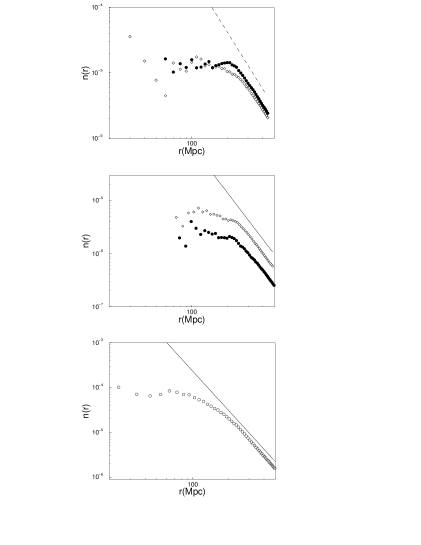
Figure 1: The radial density $n(r)$ from the vertex for a) Abell catalog Postman sample, north (diamonds) and south (filled circles) b) Abell catalog BS83 sample north (diamonds) and south (filled circles) c) ACO catalog sample (empty circles).

In Fig.1 we see that the range of scale, over which we can measure $n(r)$, is quite small ($\approx 50h^{-1}Mpc$) and in our opinion is not enough to recover the average behaviour of the density.

The study the properties of cluster spatial distribution requires an almost complete sample; then it is necessary to exclude or correct the incompleteness region. One way to obtain this in the standard approach is to assume an homogeneous distribution of clusters up to the sample limits. The observed distribution in the redshift space is then weighted with a selection function $p(z)$, that is the ratio between the observed counts of clusters in the volume $dV(z)$ at redshift $z$ and those expected from an homogeneous distribution. In our analysis, we want to avoid any assumption on the distribution itself and for this reason we will limit our analysis up to a depth corresponding to the beginning of the incompleteness region, without correcting by means of any selection function.

Another selection effect must be taken in account, regarding to the observed depletion of the surface mean density of clusters at low galactic latitude (to $|b|\mathrel{\hbox to0.0pt{\lower 3.0pt\hbox{$\mathchar 536\relax$}\hss}\raise 2.0pt\hbox{$\mathchar 316\relax$}}30^{\circ}$). This is probably due to obscuration and confusion with high-density regions of stars of our galaxy ( [26]). As in the case of redshift incompleteness, one way to overcome this incompleteness is to weigh the observed distribution with a latitude selection function $P(b)$, that is the ratio between observed surface cluster density at latitude $b$ and the expected from an homogeneous one. The normalization of this selection function is arbitrary, because it depends from the real density. Another way is to limit the sample to high galactic latitude region. We will adopt this standard procedure (i.e. $|b|\geq 30^{\circ}$ for Abell catalog and $b<-20^{\circ}$ for ACO), that has no assumptions with only the inconvenient to slightly limit the sample.

For the Postman sample [7] the distance of completeness is estimated to be roughly $230h^{-1}Mpc$ corresponding to $z\leq 0.08$, for the BS83 sample the same distance, while for ACO sample is $\approx 150h^{-1}Mpc$. All these limits have been estimated from the behaviour of the density versus the distance (Fig. 1).

4 Properties of fractal distributions

In this section we mention the essential properties of fractal structures because they will be necessary for the correct interpretation of the statistical analysis. However in no way these properties are assumed or used in the analysis itself. A fractal consists of a system in which more and more structures appear at smaller and smaller scales and the structures at small scales are similar to the ones at large scales. The self similarity of these structures is then incompatible with analyticity. Standard mathematical tools based on analytical functions can not characterize these distributions. The first quantitative description of these forms is the metric dimension. One way to determine it, is the mass-length method. Starting from an point occupied by an object, we count how many objects $N$ (”mass”) are present within a volume of linear size $r$ (”length”) ( [51]):

$$N(r)=B\cdot r^{D}$$ (3)

$D$ is the fractal dimension and characterizes in a quantitative way how the system fills the space. The prefactor $\>B$ depends to the lower cut-offs of the distribution; these are related to the smallest scale above which the system is self-similar and below which the self similarity is no more satisfied. In general we can write:

$$B=\frac{N_{*}}{{r_{*}}^{D}}$$ (4)

where $r_{*}$ is this smallest scale and $N_{*}$ is the number of object up to $r_{*}$. For a deterministic fractal this relation is exact, while for a stochastic one it is satisfied in an average sense.

Eq.(3) corresponds to a smooth convolution of real $N(r)$, that is a very fluctuating function; a fractal is, in fact, characterized by large fluctuations and clustering at all scales. We stress that eq. (3) is valid in general; for an homogeneous distribution, for example, one has $D=3$.

From eq.(3), we can compute the average density $\><n>$ for a sample of radius $\>R_{s}$ which contains a portion of the structure with dimension $D$. The sample volume is assumed to be a sphere ($\>V(R_{s})=(4/3)\pi R_{s}^{3}$) and therefore

$$<n>=\frac{N(R_{s})}{V(R_{s})}=\frac{3}{4\pi}BR_{s}^{-(3-D)}$$ (5)

If the distribution is homogeneous, $D=3$ and the average density is constant and independent from the sample volume; for a fractal, the average density depends explicitly on the sample size $\>R_{s}$ and it is not a meaningful quantity. It is a decreasing function of the sample size and $<n>\rightarrow 0$ for $R_{s}\rightarrow\infty$. It is important to note that eq. (3) holds from every point of the system, when considered as the origin. This feature is related to the non-analyticity of the distribution. In a fractal distribution every observer is equivalent to any other one, i.e. it holds the property of local isotropy around any observer ( Sylos Labini 1994 [52]). We can define the conditional density from an occupied point $i$ as:

$$\Gamma(r)_{i}=S(r)^{-1}\frac{dN(r)}{dr}=\frac{D}{4\pi}Br^{-(3-D)}$$ (6)

where $\>S(r)$ is the area of a spherical shell of radius $\>r$. $\Gamma(r)_{i}$ is then the density at distance $r$ from the $i-th$ point in a shell of thickness $dr$. As for eq.(3), eq.(6) corresponds to a smooth convolution of fluctuating quantity, i.e. the conditional density from one element of the distribution. Usually the exponent that defines the decay of the conditional density $(3-D)$ is called the codimension and it corresponds to the exponent $\>\gamma$ of the galaxy distribution.

5 The conditional average density

The correlation function suitable to study homogeneous and inhomogeneous distribution is described by ( [16]; CP92)

$$G(r)=<n(\vec{r}+\vec{r}_{i})n(\vec{r}_{i})>_{i}\approx r^{-\gamma}$$ (7)

where the exponent $\>\gamma=3-D$ (in 3-dimensional space)(Eq. 6) and the index $i$ of the average means that this is performed on all the occupied points $r_{i}$ of the system. If the sample is homogeneous,$D=3$, $\>G(r)\approx<n>^{2}$ and then is constant; if the sample has correlations on all scales, it is fractal, $D<3$, $\>\gamma>0$ and $\>G(r)$ is a power law. For a more complete discussion we refer the reader to CP92. We can normalize the $G(r)$ to the size of the sample under analysis and define, following CP92:

$$\Gamma(r)=\frac{<n(\vec{r}+\vec{r}_{i})n(\vec{r}_{i})>_{i}}{<n>}=\frac{G(r)}{<n>}$$ (8)

where $\><n>$ is the average density of the sample. This normalization does not introduce any bias even if the average density is sample-depth dependent, as in the case of fractal distributions (Eq.5), because it represents only an overall normalizing factor. The $\Gamma(r)$ (Eq. 8) can be computed by the following expression

$$\Gamma(r) = \frac{1}{N}\sum_{i=1}^{N}\frac{1}{4\pi r^{2}\Delta r}\int_{r}^{r+\Delta r}n(\vec{r}_{i}+\vec{r^{\prime}})d\vec{r^{\prime}}=$$ (9)

$$=\frac{1}{N}\sum_{i=1}^{N}\Gamma(r)_{i}=\frac{D}{4\pi}Br^{3-D}$$

where $N$ is the number of objects in the sample. This is called the conditional average density (CP92). $\Gamma(r)$ is the average of $\Gamma(r)_{i}$ and hence it is a smooth function away from the lower and upper cutoffs of the distribution ($r_{*}$ and the dimension of the sample). From eq.(9) we see that $\Gamma(r)$ is independent from the sample size, depending only by the intrinsic quantities of the distribution ($B$ and $D$). It is also very useful to use the average density

$$\Gamma^{*}(r)=\frac{3}{4\pi r^{3}}\int_{0}^{r}4\pi r^{\prime 2}\Gamma(r^{\prime})dr^{\prime}$$ (10)

This function produce an artificial smoothing of $\Gamma(r)$ function, but it correctly reproduces global properties (CP92).

As we said, $\Gamma(r)$ (and $\Gamma^{*}(r)$) is the average density computed in spherical shell. In such a way we eliminate from the statistics the points for which a sphere of radius r is not fully included within the sample boundaries. This prescription allows us to avoid any weighting scheme, i.e. any assumption in the treatment of the boundaries conditions. Of course in doing this, we have a smaller number of points and we stop our analysis at a smaller depth than that of other authors ( [5], [7], [49], [29]) In fact, we have to limit our analysis to an effective depth $R_{s}$ that is of the order of the radius of the maximum sphere fully contained in the sample volume (CP92; see also [48]). We have studied the behavior of $\>\Gamma(r)$ and $\>\Gamma^{*}(r)$ in the samples of Table 1.

Sample	N	$\Omega$	$<n>$	$d_{lim}$	$R_{s}$	$r_{0}$
		$sr$	$h^{3}Mpc^{-3}$	$(h^{-1}Mpc)$	$(h^{-1}Mpc)$	$(h^{-1}Mpc)$
BS83 sub north	$53$	$3.1$	$4.2\cdot 10^{-6}$	$230$	$70$	$27\pm 2$
Postman s.s. north	$120$	$3.1$	$9.5\cdot 10^{-5}$	$230$	$70$	$26\pm 2$
Postman s.s.south	$88$	$1.7$	$1.3\cdot 10^{-5}$	$230$	$53$	$17\pm 2$
ACO sub	$91$	$2.2$	$3.7\cdot 10^{-5}$	$150$	$50$	$17\pm 1$

Table 1: features of the various samples analyzed; column I: the catalog from which the sample has been extracted; column II: number of clusters in the sample; column III: solid angle of the sample; column IV: density of the sample; column V: sample extension; column VI: radius of the maximum sphere fully included; column VII: the correlation length

The results are shown in Fig.2. In Fig2a we have reported $\Gamma^{*}(r)$ for the north and south galactic part of Postman statistical subsample.

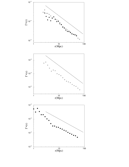
Figure 2: The behaviour of the conditional density $\Gamma(r)$ and average conditional density $\Gamma^{*}(r)$ for a) Abell catalog ,Postman sample respectively north (diamonds) and south galactic parts (filled circles) b) Abell catalog ,BS83 sample north galactic part (diamonds), c) ACO catalog sample (filled circles). $\Gamma(r)$, $\Gamma^{*}(r)$ are power law up to the radius of the greatest sphere fully included in the sample. The reference line has slope $\gamma\approx 1$

The south galactic part has a smaller solid angle with respect the north one and by consequence a smaller $R_{s}$. A well defined power law behavior is detected up to the sample limit without any tendency towards homogenization. The codimension is, with good accuracy

$$\gamma=3-D\approx 1.0\pm 0.1$$ (11)

so that $\>D\approx 2.0\pm 0.1$ up $\approx 70h^{-1}Mpc$ for the north part and up to $\approx 50h^{-1}Mpc$ for the south. The result is in good agreement with those from BS83 sample (Fig.2b). The north galactic part is fractal with dimension $D\approx 1.7\pm 0.2$ up to $r\approx 70h^{-1}Mpc$. We have not reported the analysis for the BS83 south galactic part, because it gives a very noisy result, due to the very poor statistics of the sample. The lower statistics of the BS83 sample with respect Postman one is also the reason for the little difference in the estimation of the fractal dimension $D$ of the two samples. We note that the codimension $\gamma$ for these samples has a lower value with respect the standard determination; we refer the reader to next section for a explanation of this effect. In Fig.2c we show the results from ACO sample. The $\Gamma(r)$ is a power law with exponent $D\sim 2.0\pm 0.1$ up to $\approx 50h^{-1}Mpc$. The fluctuations at $r<10h^{-1}Mpc$ are due to the fact that these distances are of the order of the minimum average distance between clusters ($\approx 15h^{-1}Mpc$ for Postman and BS83 and $\approx 8h^{-1}Mpc$ for ACO sample), so that we can then interpret them as a effect of poor statistic. In the correct regime, at distances $>10h^{-1}Mpc$, where the samples are statistically significative, the slope of $\Gamma(r)$ is almost the same for the Postman sample and for the ACO and, with a slight difference because the poor statistics, for the BS83 sample. All the samples investigated have, then, consistent statistical properties, i.e. they show a clear behaviour of the correlation function. A power law behaviour corresponds to long range correlations, which cannot be produced by random incompleteness in the sample, if they are not present. Long range correlations (fractal) can be only destroyed by incompleteness, but not produced by it.

Hence the samples show well defined statistical properties, i.e. they are statistically fair samples; the results of the analysis is that they are not homogeneous samples, but, on the contrary, fractal.

6 $\>\xi(r)$ analysis

CP92 clarify some crucial points of the standard CF analysis, and in particular they discuss the meaning of the so-called ”correlation length” $\>r_{0}$ found with the standard approach ( [21]) and defined by the relation:

$$\xi(r_{0})=1$$ (12)

where

$$\xi(r)=\frac{<n(\vec{r_{i}})n(\vec{r_{i}}+\vec{r})>_{i}}{<n>^{2}}-1$$ (13)

is the two point correlation function used in the standard analysis. As we said, if the average density is not a well defined intrinsic property of the system, the analysis with $\xi(r)$ gives spurious results. In particular, if the conditional density $\Gamma(r)$ (or $\Gamma^{*}(r)$) is a power law, the system is fractal and the average density is simply related to the sample size. In this case, if one derives a correlation length $r_{0}$, comparing the average density-density correlation to the square of average density, one obtains simply a fraction of the effective sample radius $R_{s}$. In other words, if a system has a correlation function $\Gamma(r)$ that is a power law, the system is self-similar and it has no reference values (like the average density) with respect to which one can define what is big or small. Hence, computing a correlation length with respect the average density is meaningless. As pointed out in Baryshev et al. 1994 [1], this is true also for a system that has a characteristic length, as for example a system with correlation function $\Gamma(r)=\Gamma_{0}e^{-r/r_{0}}$. In this case, the characteristic length $r_{0}$ is related to the behaviour of the function and not the prefactor $\Gamma_{0}$; the characteristic length is not defined by the condition $\Gamma(r_{0})=1$.

Following CP92, the expression of the $\>\xi(r)$ in the case of fractal distribution, is:

$$\xi(r)=((3-\gamma)/3)(r/R_{s})^{-\gamma}-1$$ (14)

where $\>R_{s}$ (the effective sample radius) is the depth of the spherical volume where one computes the average density from Eq. (5). From Eq. (14) it follows that

i.) the so-called correlation length $\>r_{0}$ (defined as $\>\xi(r_{0})=1$) is a linear function of the sample size $\>R_{s}$

$$r_{0}=((3-\gamma)/6)^{\frac{1}{\gamma}}R_{s}$$ (15)

and hence it is a quantity without any correlation meaning but it is simply related to the sample size.

ii.) the amplitude of the $\xi(r)$ is:

$$A(R_{s})=((3-\gamma)/3)R_{s}^{\gamma}$$ (16)

iii.) $\>\xi(r)$ is a power law only for

$$((3-\gamma)/3)(r/R_{s})^{-\gamma}>>1$$ (17)

hence for $\>r\mathrel{\hbox to0.0pt{\lower 3.0pt\hbox{$\mathchar 536\relax$}\hss}\raise 2.0pt\hbox{$\mathchar 316\relax$}}r_{0}$: for larger distances there is a clear deviation from a power law behavior due to the definition of $\>\xi(r)$. However usually $\xi(r)$ is fitted with a power law in the range $0.5r_{0}\mathrel{\hbox to0.0pt{\lower 3.0pt\hbox{$\mathchar 536\relax$}\hss}\raise 2.0pt\hbox{$\mathchar 316\relax$}}r\mathrel{\hbox to0.0pt{\lower 3.0pt\hbox{$\mathchar 536\relax$}\hss}\raise 2.0pt\hbox{$\mathchar 316\relax$}}2r_{0}$. The result is one obtains a greater exponent than $3-D$. This is the reason why the usual estimation of the exponent $\gamma$ of $\xi(r)$ is $\approx 1.7$, different from $\gamma\approx 1$, corresponding to $D\approx 2$, that we found by mean of the $\Gamma(r)$ analysis. Moreover we point out that there is another spurious effect in the calculation of the $\xi(r)$. The $\xi(r)$ is estimated by means of the expression

$$\xi(r)=\frac{N_{dd}(r)}{N_{pp}(r)}-1$$ (18)

where $N_{dd}(r)$ is the number of data pairs at separation $r$ and $N_{pp}(r)$ is the number of pairs at separation $r$ for a random distribution with the same density and geometry of the survey. Eq.(18) corresponds to compute the density- density correlation not only in spheres fully contained in the sample volume, but also in portions of sphere. This produce an artificial homogenization, for distances $r$ greater than the radius of the greatest sphere fully contained in the sample. For these separations, in fact, the density -density correlation is, of course, computed only in portions of sphere and this corresponds to assume that the density, found in the portion, is the same in the all solid angle. To avoid this effect, we have computed the $\xi(r)$ only up to $R_{s}$. We have studied the $\>\xi(r)$ in our samples of clusters. In fig. 3

Figure 3: The $\xi(r)$ function for the a) Postman sample (north) (filled circles) b) Postman sample (south) (filled circles) and ACO (diamonds). The reference line is the functional form of eq.(14) with $\gamma\approx 1$

we have reported the $\xi(r)$ for the Postman sample (north and south) and for the ACO sample. We have fitted the experimental points with the functional form of eq.(14). We found that $\>\gamma\approx 1$ for the all samples analyzed. The corresponding $r_{0}$ are reported in the Table 1; for the Postman sample north we found $r_{0}\approx 26\pm 2$ and for BS83 sample $r_{0}\approx 27\pm 2$ These two samples have the same $r_{0}$ as we expect, noting that they have the same $R_{s}$. The values found are in agreement with eq.(15). The same conclusions hold for the other two samples: Postman south and ACO. Both of them have $R_{s}$ ($\approx 50h^{-1}Mpc$) and the same $r_{0}$ ($\approx 17h^{-1}Mpc$), according to eq.(15). In conclusion $r_{0}$ is simply a fraction of the sample size $R_{s}$, without any physical meaning for the properties of the samples.

7 Conclusion

We have analyzed the properties of the various Abell/ACO cluster samples. The statistical analysis, performed without any a priori assumptions, shows that Abell samples are fractal with fractal dimension $D\approx 2$ for Postman sample and for BS83 sample up to $\approx 70h^{-1}Mpc$ and for ACO sample up to $\approx 50h^{-1}Mpc$. The different limiting distance of the analysis in the various samples corresponds to the radius of the greatest sphere fully included in the sample, that is different in the various samples. This limitation allows us to avoid any weighting schemes or assumptions in the analysis. The result of the statistical analysis is that no tendency towards homogenization is detected within the sample limits. The so-called correlation length $r_{0}$ derived from the $\xi(r)$ analysis, is simply directly proportional to the sample size $R_{s}$ and then, it is meaningless with respect the correlation properties of the system.

This result is in agreement with the correlation analysis, performed measuring the conditional average density, $\Gamma(r)$, that is a power law (${\it fractal}$) within the sample limits. Moreover our results on cluster samples are in remarkable agreement with the same analysis performed on various galaxy redshift surveys (CfA1, Perseus Pisces, LEDA, ESP) as one expects for a fractal distribution of galaxy and clusters. The mismatch between galaxy and cluster correlation is just due to the mathematical inconsistency of the use of $\xi(r)$ and the correct analysis, in terms of $\Gamma(r)$ and $\Gamma^{*}(r)$, shows that correlations of clusters are just the continuation at larger scales of galaxy correlations. We conclude that galaxies and clusters are two different representations of the same self similar structure.

Galaxy clusters extend the correlations of galaxies to deeper depth. In this respect cluster distribution represents a coarse grained representation of galaxies; it is the same self-similar distribution, but sampled with a large scale resolution. i.e. considering a cluster of galaxies as a single object, without distinguish the structure in it. Hence, we can study the clusters distribution simply performing a coarse graining on galaxy distribution. Usually clusters are identified with some criteria, that are different according to different observers. On the contrary, in this way, we can make the analysis independently from the definition of cluster, supercluster etc., but one has to know the complete galaxy survey over which performing the coarse graining procedure. The same considerations hold, of course, for the void distribution: the void distribution is, in fact, just the complement of the matter one. In conclusion, our methods have the advantage to be independent from the nature of the distribution considered, and they gives a quantitative way to detect self similar properties, whether they exist, at different scales.

Acknowledgements

We thank prof. L. Pietronero for useful discussions and enlightening suggestions. We are also grateful to A.Amendola, A.Gabrielli, H. Di Nella, H.Andernach and R. Cafiero; to R. Capuzzo Dolcetta for useful comments and collaboration. This work has been partially supported by the Italian Space Agency (ASI).

References

- [1] Baryshev, Y. et al., 1994, Vistas in Astronomy, 38, N.4, 419
- [2] Tully B. R., , Astrophys.J 303 , (1986) 25
- [3] Tully, B. R., Scaramella, R., Vettolani G., Zamorani G., Astrophys.J 388, (1992) 9
- [4] Einasto J. et al., Mon.Not.R.Acad.Soc 269, (1994) 301
- [5] Bahcall N. A. & Soneira R. M., 1983, ApJ, 270, 20
- [6] Batusky D. J. & Burns,J. O., Astrophys.J 299, (1985) 5
- [7] Postman M., Huchra J. P., & Geller M. J., Astrophys.J 384, (1992) 404
- [8] Zucca E., Scaramella, R., Vettolani G., Zamorani G., Astrophys.J 407, (1992) 470
- [9] Kauffmann G. &, Fairall A. P., Mon.Not.R.Acad.Soc 248, (1991) 313
- [10] Haque-Copilah, S. & Basu, D., 1994, Astronomical Society of the Pacific., 106, 67
- [11] Lindner U., Einasto J., Einasto, M., Wolfram F., Klaus F., Tago E., Astron. Astrophys., 301, (1995) 329
- [12] Hopp, U., 1994, Proceedings of the ESO OHP workshop ”Dwarf Galaxies”
- [13] Peebles P. J. E., Schramm, D. N., Turner, E. L., Kron, R. G. 1991, Nature, 352, 769
- [14] Peebles P. J. E., 1993, Principles of physical cosmology, Princeton Univ. Press
- [15] Peebles P. J. E., Schramm, D. N., Turner, E. L., Kron, R. G. 1994, Scientific American, 316, 26
- [16] Pietronero L., 1987, Physica A, 144, 257
- [17] Coleman P.H., Pietronero, L., Sanders R.H., 1988, A & A Lett., 200, L32
- [18] Coleman P.H. & Pietronero, L., 1992, Phys. Reports, 213, 311
- [19] Kirshner R. P., Olmer A. Jr., Schecter P., L., 1978, AJ, 83, 1549
- [20] Peebles P. J. E., 1980, Large Scale Structure of the Universe , Princeton Univ. Press
- [21] Davis, M. & Peebles, P. J., 1983, ApJ, 267, 465
- [22] Shanks, T. et al. 1983, ApJ, 274, 529
- [23] De Lapparent, V., Geller M., J., Huchra J.P., 1988, ApJ, 332 , 44
- [24] Abell, G. O., 1958, ApJS, 3, 211
- [25] Klypin, A. A. & Kopylov, A.I., Soviet Astr. Lett., 9, (1983) 41
- [26] Bahcall N. A., Astron. Astrophys. Ann. Rev., 26, (1988) 63
- [27] Abell G. O., Corwin H.G. Jr., Olowin R. P., 1989, ApJS, 70, 1
- [28] Huchra J. P., Henry J. P., Postman M., Geller M.J., Astrophys.J. 365, (1990), 66
- [29] Cappi A. & Maurogordato S., Astron.Astrophys. 259, (1992) 423
- [30] Sutherland W. J., Mon.Not.R.Acad.Soc , 234, (1988) 159
- [31] Dekel A., Blumenthal, G. R., Primack, J. R., Olivier S., Astrophys.J., 338, (1989) L5
- [32] Sutherland W. J & Efstathiou, G., Mon.Not.R.Acad.Soc , 248, (1991) 159
- [33] Efstathiou G., Dalton G. B., Sutherland W. J., Maddox S. J., Mon.Not.R.Acad.Soc, 257, (1992) 125
- [34] Van Harlem M. P., (1996), preprint
- [35] Groth, E. & Peebles, P.J. E., 1977, ApJ, 217, 385
- [36] Peebles P. J. E., 1993, Principles of physical cosmology, Princeton Univ. Press
- [37] Bahcall N. A. & Burgett W. S., 1986 Astrophys.J., 300, (1986) L35
- [38] Bahcall N. & West M.J. Astrophys.J. 392, (1992) 419
- [39] Bahcall N. A. & Cen R., Astrophys.J. (1994) ??
- [40] Szalay A. S. & Schramm D. N., Nature, 314, (1985) 718
- [41] Huchra J. P., Davis M., Latham D., Tonry J., 1983, ApJS, 52, 89
- [42] Sylos Labini F., Montuori M., Pietronero L., 1996a, Physica A, 230, 336
- [43] Sylos Labini F., Gabrielli A., Montuori M., Pietronero L., 1996b, Physica A, 226, 195
- [44] Sylos Labini F. & Pietronero L., 1996, ApJ, 468, Sept. 20
- [45] Sylos Labini F. & Amendola L., 1996 ApJL, 468, L1
- [46] Di Nella H., Montuori M., Paturel G., Pietronero L., Sylos Labini F., 1996, A & A Lett., 308, L33
- [47] Amendola L., Di Nella H., Montuori M., Sylos Labini F., 1996 preprint
- [48] Sylos Labini F., Montuori M., Pietronero L., 1997, preprint
- [49] Plionis M., Valdarnini R., Jing Y. P., 1992, ApJ, 398, 12
- [50] Plionis M. & Valdarnini R., 1991, MNRAS, 249, 46
- [51] Mandelbrot, B. B., 1982, The fractal geometry of the nature, Freeman San Francisco
- [52] Sylos Labini F., 1994 ApJ, 433, 464