Abstract

We present a new data analysis method to study rectangular $T^{3}$ “small universes” with one or two of its dimensions significantly smaller than the present horizon (which we refer to as $T^{1}$- and $T^{2}$-models, respectively). We find that the 4 year $COBE$/DMR data set a lower limit on the smallest cell size for $T^{1}$- and $T^{2}$-models of 3000$h^{-1}$Mpc, at 95% confidence, for a scale invariant power spectrum ($n$=1).

CONSTRAINING TOPOLOGY WITH THE CMB

¹Max-Planck-Institut für Astrophysik, Garching, Germany. ²Lawrence Berkeley National Laboratory, Berkeley, USA. ³Russian Academy of Sciences, Moscow, Russia.

1 Introduction

In the past few years, mainly after the discovery of CMB anisotropies by $COBE$/DMR [11], the study of the topology of the universe has become an important problem for cosmologists and some hypotheses, such as the “small universe” model [4], have received considerable attention. From the theoretical point of view, it is possible to have quantum creation of the universe with a multiply-connected topology [16]. From the observational side, this model has been used to explain the “observed” periodicity in the distributions of quasars [7] and galaxies [1].

Almost all work on “small universes” has been limited to the case where the spatial sections form a rectangular basic cell with sides $L_{x},L_{y},L_{z}$ and with opposite faces topologically connected, a topology known as toroidal. The three-dimensional cubic torus $T^{3}$ is the simplest model among all possible multiply-connected topologies, in which all three sides have the same size $L\equiv L_{x}=L_{y}=L_{z}$. In spite of the fact that cubic $T^{3}$-model has been ruled out by $COBE$ results [2, 8, 12, 13, 14], the possibility that we live in a universe with a more anisotropic topology, such as a rectangular torus $T^{3}$, is an open option that has not been ruled out yet. For instance, if the toroidal model is not a cube, but a rectangle with sides $L_{x}\neq L_{y}\neq L_{z}$ and with one or two of its dimensions significantly smaller than the horizon $R_{H}$ ($\equiv 2cH_{0}^{-1}$), this small rectangular universe cannot be completely excluded by any of the previous analyses: constraints from the DMR data merely require that at least one of the sides of the cell be larger than $R_{H}$.

As pointed out by [5] and [13], if the rectangular $T^{3}$-universe has one of the cell sizes smaller than the horizon and the other two cell sizes are of the order of or larger than the horizon (for instance, $L_{z}\ll R_{H}$ and $L_{x},L_{y}\mathrel{\hbox to0.0pt{\lower 3.0pt\hbox{$\mathchar 536\relax$}\hss}\raise 2.0pt\hbox{$\mathchar 318\relax$}}R_{H}$), the values of $\delta T/T$ are almost independent of the $z$-coordinate, i.e., the large scale CMB pattern shows the existence of a symmetry plane formed by the $x$ and $y$-axes; and if it has two cell sizes smaller than the horizon and the third cell size is of the order of or larger than the horizon (for instance, $L_{x},L_{y}\ll R_{H}$ and $L_{z}\mathrel{\hbox to0.0pt{\lower 3.0pt\hbox{$\mathchar 536\relax$}\hss}\raise 2.0pt\hbox{$\mathchar 318\relax$}}R_{H}$), the temperatures $\delta T/T$ are aproximately independent of both $x$ and $y$, i.e., the CMB pattern shows the existence of a symmetry axis: values of $\delta T/T$ are almost constant along rings around the $z$-axis. We call the former case a $T^{1}$-model because the spatial topology of the universe becomes just $T^{1}$ in the limit $L_{x},L_{y}\to\infty$ with $L_{z}$ being fixed. The later case is denoted a $T^{2}$-model for the same reason (the corresponding limit is $L_{z}\to\infty$ with $L_{x},L_{y}$ being fixed). See Figures 1A (upper left) and 1B (upper right).

Our goal is to show that the $COBE$/DMR maps have the ability to test and rule out $T^{1}$- and $T^{2}$-models. We use a new approach to study these models in which we constrain their sizes by looking for the symmetries that they would produce in the CMB, obtaining strong constraints from the 4 year $COBE$/DMR data.

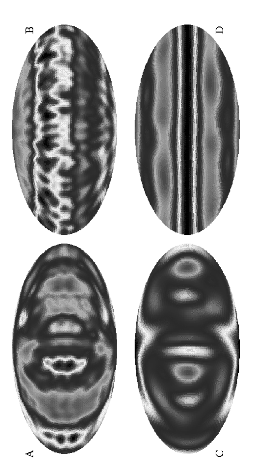
Figure 1: Simulated sky maps for the $T^{1}$- and $T^{2}$-models and their $S$-maps. (A) $T^{1}$-model with dimensions ($L_{x},L_{y},L_{z}$) = $R_{H}$(3,3,0.3); (B) $T^{2}$-model with dimensions ($L_{x},L_{y},L_{z}$) = $R_{H}$(0.3,0.3,3); (C) $S$-map of the $T^{1}$-model shown in ($A$); (D) $S$-map of the $T^{2}$-model shown in ($B$). Both models are plotted in galactic coordinates and have a scale invariant power spectrum ($n$=1).

2 The method

The analysis of $T^{1}$- and $T^{2}$-models is not an easy task, since there are infinitely many combinations of different cell sizes and cell orientations. In order to study these models, we choose a statistic in which we calculate the function $S(\hat{\bf n}_{i})$ defined by [3]

$$S(\hat{\bf n}_{i})\equiv\frac{1}{N_{pix}}\sum_{j=1}^{N_{pix}}\frac{[\frac{\delta T}{T}(\hat{\bf n}_{j})-\frac{\delta T}{T}(\hat{\bf n}_{ij})]^{2}}{\sigma(\hat{\bf n}_{j})^{2}+\sigma(\hat{\bf n}_{ij})^{2}},$$ (1)

where $N_{pix}$ is the number of pixels that remain in the map after the Galaxy cut has taken place, $\hat{\bf n}_{ij}$ denotes the reflection of $\hat{\bf n}_{j}$ in the plane whose normal is $\hat{\bf n}_{i}$, i.e.,

$$\hat{\bf n}_{ij}=\hat{\bf n}_{j}-2(\hat{\bf n}_{i}\cdot\hat{\bf n}_{j})\hat{\bf n}_{i},$$ (2)

and $\sigma(\hat{\bf n}_{j})$ and $\sigma(\hat{\bf n}_{ij})$ are the r.m.s. errors associated with the pixels in the directions $\hat{\bf n}_{j}$ and $\hat{\bf n}_{ij}$. $S(\hat{\bf n}_{i})$ is a measure of how much reflection symmetry there is in the mirror plane perpendicular to $\hat{\bf n}_{i}$. The more perfect the symmetry is, the smaller $S(\hat{\bf n}_{i})$ will be. When we calculate $S(\hat{\bf n}_{i})$ for all 6144 pixels at the positions $\hat{\bf n}_{i}$, we obtain a sky map that we refer to as an $S$-map. This sky map is a useful visualization tool and gives intuitive understanding of how the statistic $S(\hat{\bf n}_{i})$ works.

In order to better understand $S(\hat{\bf n}_{i})$, we first consider the simple model of a $T^{1}$-universe with $L_{z}\ll R_{H}$. For this specific model, the values of $\delta T/T$ are almost independent of the $z$-coordinate, so we have almost perfect mirror symmetry about the $xy$-plane or, in spherical coordinates, $\delta T/T(\theta,\phi)\approx\delta T/T(\pi-\theta,\phi)$. When $\hat{\bf n}_{i}$ points in the direction of the smallest cell size (i.e., in the $z$-direction), we have $S(\hat{\bf n}_{i})\approx$ 1; otherwise, $S(\hat{\bf n}_{i})>$ 1. An $S$-map for a $T^{1}$-model ($L_{x},L_{y},L_{z}$) = $R_{H}$(3,3,0.3) can be seen in Figure 1C (lower left). Notice in this plot that the direction in which the cell is smallest can be easily identified by two “dark spots” at $\hat{\bf n}_{i}\approx\hat{\bf z}$ and $\hat{\bf n}_{i}\approx-\hat{\bf z}$. For $T^{2}$-models, the only difference will be that in the place of the two “dark spots”, we have a “dark ring” structure in the plane formed by the two small directions. See Figure 1D (lower right), an $S$-map of the $T^{2}$-model ($L_{x},L_{y},L_{z}$) = $R_{H}$(0.3,0.3,3).

From the two $S$-maps, we can infer two important properties: first, the direction in which the $S$-map takes its minimum value, denoted $S_{\circ}$, is the direction in which the universe is small. For a large universe such as $L_{x},L_{y},L_{z}\gg R_{H}$, the $S_{\circ}$-directions obtained from different realizations are randomly distributed in the sky. Secondly, the distribution of $S_{\circ}$-values changes with the cell size, i.e., as the universe becomes smaller, the values of $S_{\circ}$ decrease. From the definition of the $S$-map, it is easy to see that the value of $S_{\circ}$ is independent of the cell orientation. In other words, if we rotate the cell, we will just be rotating the $S$-map, leaving its minimum value $S_{\circ}$ unchanged.

From here on, we will present our results in terms of the cell sizes $R_{x}$, $R_{y}$ and $R_{z}$, usually sorted as $R_{x}\leq R_{y}\leq R_{z}$ and defined as $R_{x}\equiv L_{x}/R_{H}$, $R_{y}\equiv L_{y}/R_{H}$ and $R_{z}\equiv L_{z}/R_{H}$. We remind the reader that the results are identical for all six permutations of $R_{x}$, $R_{y}$ and $R_{z}$.

3 Data Analysis

Figure 2: Cumulative probability distribution of $S_{\circ}$ for $T^{1}$- and $T^{2}$-models obtained from Monte Carlo simulations. A, left plot: Simulations for $T^{2}$-universes with dimensions ($R_{x},R_{y},R_{z}$) = (0.5,0.5,3) or dot-dashed line, (0.6,0.6,3) or dashed line, and (0.7,0.7,3) or dotted line. B, right plot: Simulations for $T^{1}$-universes with dimensions ($R_{x},R_{y},R_{z}$) = (0.5,3,3) or dot-dashed line, (0.6,3,3) or dashed line, and (0.7,3,3) or dotted line. In both pictures the model ($R_{x},R_{y},R_{z}$) = (3,3,3) is represented by a solid line, $S_{\circ}^{DMR}$ = 2.59 (vertical straight line) and the horizontal solid lines indicate the confidence levels of 95%, 90% and 68% (from top to bottom).

If the density fluctuations are adiabatic and the Universe is spatially flat, the Sachs-Wolfe fluctuations in the CMB are given by [10]

$$\frac{\delta T}{T}(\theta,\phi)=-\frac{1}{2}\frac{H_{0}^{2}}{c^{2}}\sum_{\bf k}\frac{\delta_{\bf k}}{{k}^{2}}e^{i{\bf k}\cdot{\bf r}},$$ (3)

where r is the vector with length $R_{H}\equiv 2cH_{0}^{-1}$ that points in the direction of observation ($\theta,\phi$), $H_{0}$ is the Hubble constant (written here as $100h$ km s^-1 Mpc^-1) and $\delta_{\bf k}$ is the density fluctuation in Fourier space, with the sum taken over all wave numbers k.

In a Euclidean topology the universe is isotropic, and the sum in (3) is normally replaced by an integral. However, in a toroidal universe this is not the case. In this model, only wave numbers that are harmonics of the cell size are allowed. As a result, we have a discrete k spectrum [6, 15]

$${\bf k}=\frac{2\pi}{R_{H}}\left(\frac{p_{x}}{R_{x}},\frac{p_{y}}{R_{y}},\frac{p_{z}}{R_{z}}\right),$$ (4)

where $p_{x}$, $p_{y}$ and $p_{z}$ are integers.

From equation (3), we can construct simulated skies by calculating [3]

$$\frac{\delta T}{T}(\theta,\phi)\propto\sum_{p_{x},p_{y},p_{z}}\left[g_{1}\cos(2\pi\gamma)+g_{2}\sin(2\pi\gamma)\right]\alpha^{\frac{n-4}{4}}e^{-(R_{H}\Theta k_{\perp})^{2}/2}+n(\theta,\phi),$$ (5)

where $g_{1}$ and $g_{2}$ are two independent Gaussian random variables with zero mean and unit variance, $\gamma=\left(\frac{p_{x}}{R_{x}}x+\frac{p_{y}}{R_{y}}y+\frac{p_{z}}{R_{z}}z\right)$, $\alpha\equiv\left(\frac{p_{x}}{R_{x}}\right)^{2}+\left(\frac{p_{y}}{R_{y}}\right)^{2}+\left(\frac{p_{z}}{R_{z}}\right)^{2}\propto k^{2}$ and $n$ is the spectral index of the scalar perturbations. The term $e^{-(R_{H}\Theta k_{\perp})^{2}/2}$ represents the experimental beam function, where $k_{\perp}$ is the length of the ${\bf k}$-component perpendicular to the line of sight and $\Theta$ is the width of the Gaussian beam given by $\Theta={\rm FWHM}/\sqrt{8\ln{2}}\approx 0.43~{}{\rm FWHM}$, where FWHM is the full width of the beam at its half maximum. Finally, we model the noise $n(\theta,\phi)$ at each pixel $i$ as independent Gaussian random variables with mean $\langle n_{i}\rangle=$0 and variance $\langle n_{i}n_{j}\rangle=\sigma_{ij}\delta_{ij}$ [9].

We generate our simulated skies as standard DMR maps with 6144 pixels for $n$=1, with a Galaxy cut of 20^∘, FWHM = 7^∘, the monopole and dipole removed, add noise and normalize to $\sigma_{7^{\circ}}=34.98\mu$K (the r.m.s. value at 7^∘ extracted from our DMR map, a 4 year combined 53 plus 90 GHz map with monopole and dipole removed). Fixing a cell size, we construct a simulated sky according to (5), we smooth this once more by 7^∘ and use the statistic defined in (1) to obtain an $S$-map from which we extract its minimum value $S_{\circ}$. Repeating this procedure 1000 times, we obtain the probability distribution of $S_{\circ}$ for that fixed cell size. When we repeat this same procedure for different cell sizes, we are able to construct plots as shown in Figure 2.

In Figure 2A (left plot), we show the cumulative probability distribution of $S_{\circ}$ obtained from the Monte Carlo simulations for the cell sizes ($R_{x},R_{y},R_{z}$) = (0.5,0.5,3), (0.6,0.6,3), (0.7,0.7,3) and (3,3,3). The horizontal lines indicate the confidence levels of 95%, 90% and 68% (from top to bottom). Comparing these curves with the value $S_{\circ}^{DMR}$ = 2.59 (represented in the plot by the vertical straight line), where $S_{\circ}^{DMR}$ is the $S_{\circ}$ value extracted from our data set, we conclude that $T^{2}$-models with smallest cell sizes $R_{x},R_{y}\mathrel{\hbox to0.0pt{\lower 3.0pt\hbox{$\mathchar 536\relax$}\hss}\raise 2.0pt\hbox{$\mathchar 316\relax$}}$0.5 can be ruled out at 95% confidence. As the second cell size $R_{y}$ is increased, the curves shift to the left of the $T^{2}$-models and we can rule out $T^{1}$-models for $R_{x}\mathrel{\hbox to0.0pt{\lower 3.0pt\hbox{$\mathchar 536\relax$}\hss}\raise 2.0pt\hbox{$\mathchar 316\relax$}}$0.5 at a similar confidence level, see Figure 2B (right plot). In this plot, we show the cumulative probability distribution of $S_{\circ}$ obtained from Monte Carlo simulations for the cell sizes ($R_{x},R_{y},R_{z}$) = (0.5,3,3), (0.6,3,3), (0.7,3,3) and (3,3,3).

A more complete picture of the cell size limits is obtained when we construct a two-dimensional grid for different values of the cell sizes ($R_{x},R_{y},R_{z}$) with $R_{z}=3.0$ and $0.2<R_{x},R_{y}<3.0$ (see Figure 3). The thin-shaded, thick-shaded and grey regions correspond, respectively, to the models ruled out at 68%, 90% and 95% confidence. Notice in this plot that all contours are almost $L$-shaped, which means that, to a good approximation, the level in which a model ($R_{x},R_{y}$) is ruled out depends only on the smallest cell size, $R_{min}\equiv{\it min}\{R_{x},R_{y}\}$. We see that $R_{min}\mathrel{\hbox to0.0pt{\lower 3.0pt\hbox{$\mathchar 536\relax$}\hss}\raise 2.0pt\hbox{$\mathchar 318\relax$}}$0.5 at 95% confidence.

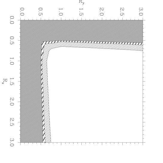
Figure 3: Grid of cumulative probability distributions of $S_{\circ}$ for $T^{1}$- and $T^{2}$-models obtained from Monte Carlo simulations. The thin-shaded, thick-shaded and grey regions correspond, respectively, to the models ruled out at 68%, 90% and 95% confidence.

4 Conclusions

We have shown that the $COBE$/DMR maps have the ability to test and rule out $T^{1}$ and $T^{2}$ topological models. We have presented a new statistic to study these anisotropic models which quantifies the “smallness” of a sky map in a single number, $S_{\circ}$, which is independent of the cell orientation, is precisely sensitive to the type of symmetries that small universes produce, is easy to work with and is easy to interpret.

From the $COBE$/DMR data, we obtain a lower limit for $T^{1}$- and $T^{2}$-models of $R_{x}\mathrel{\hbox to0.0pt{\lower 3.0pt\hbox{$\mathchar 536\relax$}\hss}\raise 2.0pt\hbox{$\mathchar 318\relax$}}$0.5, which corresponds to a cell size with smallest dimension of $L$=3000$h^{-1}$Mpc. This limit is at 95% confidence and assumes $n$=1. Since the topology is interesting only if the cell size is considerably smaller than the horizon, so that it can (at least in principle) be directly observed, these models lose most of their appeal. Since the cubic $T^{3}$ case has already been ruled out as an interesting cosmological model [2], and $T^{1}$- and $T^{2}$-models for small cell sizes are ruled out, this means that all toroidal models (cubes and rectangles) are ruled out as interesting cosmological models.

Acknowledgements.  We would like to thank Jon Aymon and Al Kogut for the help with the $COBE$ library subroutines and Max Tegmark for many useful comments on the manuscript.

References

- [1] Broadhurst, T.J., Ellis, R.S., Koo, D.C. & Szalay, A.S. 1990, Nature 343, 726
- [2] de Oliveira-Costa, A. & Smoot, G.F. 1995, Astrophys. J. 448, 447
- [3] de Oliveira-Costa, A., Smoot, G.F. & Starobinsky, A.A. 1996, Astrophys. J. 468, 457
- [4] Ellis, G.F.R. & Schreiber, G. 1986, Phys. Lett. A 115, 97
- [5] Fang, L.Z. 1993, Mod. Phys. Lett. A 8, 2615
- [6] Fang, L.Z. & Houjun, M. 1987, Mod. Phys. Lett. A 2, 229
- [7] Fang, L.Z. & Sato, H. 1985, Gen. Rel. and Grav. 17, 1117
- [8] Jing, Y.P. & Fang, L.Z. 1994, Phys. Rev. Lett. 73, 1882
- [9] Lineweaver, C. et al. 1994, Astrophys. J. 436, 452
- [10] Peebles, P.J.E. 1982, Astrophys. J. 263, L1
- [11] Smoot, G.F. et al. 1992, Astrophys. J. 396, L1
- [12] Sokolov, I.Y. 1993, JETP Lett. 57, 617
- [13] Starobinsky, A.A. 1993, JETP Lett. 57, 622
- [14] Stevens, D., Scott, D. & Silk, J. 1993, Phys. Rev. Lett. 71, 20
- [15] Zel’dovich, Ya B. 1973, Comm. Astrophys. Space Sci. 5, 169
- [16] Zel’dovich, Ya B. & Starobinsky, A.A. 1984, Sov. Astron. Lett. 10, 135