Abstract

In recent years, our knowledge of photospheric magnetic fields went through a thorough transformation—nearly unnoticed by dynamo theorists. It is now practically certain that the overwhelming majority of the unsigned magnetic flux crossing the solar surface is in turbulent form (intranetwork and hidden fields). Furthermore, there are now observational indications (supported by theoretical arguments discussed in this paper) that the net polarity imbalance of the turbulent field may give a significant or even dominant contribution to the weak large-scale background magnetic fields outside unipolar network areas. This turbulent magnetic field consists of flux tubes with magnetic fluxes below $10^{10}$ Wb ($10^{18}$ Mx). The motion of these thin tubes is dominated by the drag of the surrounding flows, so the transport of this component of the solar magnetic field must fully be determined by the kinematics of the turbulence (i.e. it is “passive”), and it can be described by a one-fluid model like mean-field theory (MFT). The recent advance in the direct and indirect observation of turbulent fields is therefore of great importance for MFT as these are the first-ever observations on the Sun of a field MFT may be applied to. However, in order to utilize the observations of turbulent fields and their large-scale patterns as a possible diagnostic of MFT dynamo models, the transport mechanisms linking the surface field to the dynamo layer must be thoroughly understood.

This paper reviews the theory of passive magnetic field transport using mostly first (and occasionally higher) order smoothing formalism; the most important transport effects are however also independently derived using Lagrangian analysis for a simple two-component flow model. Solar applications of the theory are also presented. Among some other novel findings/propositions it is shown that the observed unsigned magnetic flux density in the photosphere requires a small-scale dynamo effect operating in the convective zone and it is proposed that the net polarity imbalance in turbulent (and, in particular, hidden) fields may give a major contribution to the weak large-scale background magnetic fields on the Sun.

solar physics, magnetism

Section 1 Introduction

1.1 “Passive” Fields vs. “Active” Fields: a Historical Review

A basic rule of thumb in magnetohydrodynamics (MHD) tells us that the character of the interaction between motions and magnetic fields in a (high plasma beta) plasma is determined by the ratio of the $E_{M}$ magnetic and $E_{K}$ kinetic energy densities. If $E_{M}\ll E_{K}$ then the Lorentz force may be neglected in the equation of motion and our problem is reduced to the kinematical case. If, on the other hand, $E_{M}\gg E_{K}$ then the field will “channel” the flow and the only potential effect of the motions on the field is the generation of small-aplitude MHD waves: this is the strong field case. Finally, in the hydromagnetic case, when $E_{M}\sim E_{K}$, there is a complicated interaction of flow and magnetic field. Of course we must be aware of the fact that $\langle\mbox{\bf B}^{2}\rangle>\langle\mbox{\bf B}\rangle^{2}$ in general, so the $E_{M}$ total magnetic energy density may well exceed the energy density of the large-scale mean field. Besides, the validity of the above simple rule may possibly also be limited in two dimensions where a weaker magnetic field (consisting e.g. of a low filling factor set of strong sheets) could possibly also influence the motion, owing to the topological constraint (the flow cannot “get around” the sheets). These latter points were recently brought into focus by ? (?). Nevertheless, apart from these rather obvious caveats, the simple rule summarized above can be considered as correct. This simple notion formed the background of MHD thinking in the 1950’s and 60’s when mean-field electrodynamics and mean-field MHD were developed (?, ?, ?, ?) for the treatment of the kinematic and hydromagnetic case, respectively.

The picture however got more complicated in the period from the mid-sixties to the mid-seventies when solar observations (?, ?, ?, ?, ?, ?) and numerical experiments (?, ?) showed that in the highly conductive turbulent solar plasma the magnetic field is concentrated into strong flux tubes with very little flux in between. The $B_{\rm t}$ magnetic flux density inside the tubes is order of (or greater than) the $B_{\rm eq}$ equipartition flux density defined by

$$B_{\rm eq}^{2}/2\mu=\rho v_{\rm t}^{2}/2$$ (1)

(SI formula; $\mu$ is the permeability, $\rho$ is the density, $v_{\rm t}=\langle v^{2}\rangle^{1/2}$ with $v$ the turbulent velocity). As a consequence of this realization, flux tube theory began to develop in the 1970’s (see ?, ?, for a review of the results of this period). According to flux tube theory, the most important forces acting on a magnetic flux tube are the $F_{\rm d}$ aerodynamic drag, the $F_{\rm m}$ magnetic curvature force and the $F_{\rm b}$ buoyancy; their approximate expressions are:

$$F_{\rm b}\sim\frac{B_{\rm t}^{2}}{2\mu_{0}H_{P}}\qquad F_{\rm m}\sim\frac{B_{\rm t}^{2}}{\mu_{0}R_{\rm c}}\qquad F_{\rm d}\sim\frac{\rho v_{\rm t}^{2}}{d}$$ (2)

with $H_{P}$ the pressure scale height, $d$ the tube diameter and $R_{\rm c}$ the curvature radius; in practice, one may put $R_{\rm c}\sim l$ with $l$ the characteristic scale of the turbulence. A comparison of these expressions shows that for a sufficiently thin flux tube, with a magnetic flux $\Phi<\Phi_{\rm cr}=\mbox{min\,}\{l^{2},H_{P}^{2}\}B_{\rm eq}^{4}/B_{\rm t}^{3}$, the drag will dominate and the surrounding flow will determine the motion, while thicker tubes may move more independently of the surrounding turbulence, under the action of dynamical forces. This implies that, for a given energy density (for a given $f$ magnetic filling factor or $D$ typical tube separation), the transport of the field may be either passive, i.e. fully determined by the flow between the tubes, or active, i.e. to a large degree independent of the flow in the non-magnetic component, depending on whether the field is organized in a large number of thin fibrils or in a small number of thick flux bundles. Our classification of magnetic field types from the point of view of transport should therefore be extended into a two-dimensional scheme:
Passive Active ($d\ll l$) ($d\sim l$) Weak ($d\ll D$ or $E_{M}\ll E_{K}$) PW AW Moderate ($d\sim D$ or $E_{M}\sim E_{K}$) PM AM Strong ($E_{M}\gg E_{K}$) S
(cf. also Fig. 1). Traditional MFT, with its one-fluid approach, may be applied to passive fields, but it is clearly not applicable to the case of active fields as these would require a two-fluid description. (An interesting attempt at the construction of a more general, two-fluid MFT was made by ?, ?.)

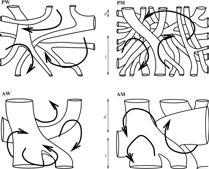
Figure 1.  : Types of magnetic field structure from the point of view of field transport. Note that “passive” (P) does not imply “kinematical”: e.g. in case PM the presence of thin flux tubes in large numbers may significantly alter the flow pattern by posing a serious obstacle in the way of the flow.

Now let us estimate the value of $\Phi_{\rm cr}$ for the solar photosphere. Using $H_{P}\sim 100$ km, $l\sim 10^{3}$ km (the granular scale) and assuming $B_{\rm t}\sim B_{\rm eq}\simeq 40$ mT we find $\Phi_{\rm cr}\sim 10^{9}$–$10^{10}$ Wb. (The assumption of $B_{\rm t}\sim B_{\rm eq}$ is to some extent validated by the observations of ?, ?.) Flux tubes with such low flux values were rarely (if ever) observed on the Sun prior to the mid-1980’s. As a consequence, all or most of the photospheric magnetic field was thought to be in active form, and, from the late 1970’s onwards, serious doubts arose concerning the relevance of MFT to the solar dynamo problem. The emphasis of research shifted to flux tube emergence calculations and numerical experiments.

The observations of the last 5–10 years have brought a fundamental change in our perception of photospheric fields; an important consequence of these new results may be a partial “rehabilitation” of MFT as the basic theory of solar activity. Because of their importance, these recent observational results will be summarized separately in the next subsection. First however we should briefly deal with a number of other objections against MFT.

Beginning with the famous paper by ? (?) on the “buoyancy problem”, evidence has been mounting for a dynamo located at the bottom of the solar convective zone or below. It is then clear that the study of magnetic field transport is crucial in understanding the cause of this spatial restriction of the dynamo mechanism as well as in relating the fields seen at the surface to the dynamo deep below. In the past, MFT dynamo models usually ignored the transport effects, except turbulent diffusion (and occasionally a phenomenological term imitating buoyancy). In fact, although some theoretical results concerning magnetic field transport were sporadically published (and will be cited in subsequent sections of this paper), this subject has only been reviewed once (?, ?), and solar applications only began in earnest in the 1980’s.

MFT’s usual limitation to the kinematical case with first order smoothing also used to be a subject of criticism. In recent years, however, a number of important papers on higher order and nonlinear effects (cf. Sects. 3.2–3.4) improved the position of MFT in this respect as well.

In summary: although MFT is certainly no wonder-drug, it is a powerful and versatile theory which is able to reproduce some basic features of solar activity (e.g. the butterfly diagram) and which should be applicable to at least one important component of the solar magnetic field: to passive fields.

1.2 The Impact of Observations

Passive fields are freely advected by turbulence, so their fluctuating component, the turbulent field must have a characteristic scale or correlation length not exceeding that of the turbulence. Numerical experiments and turbulence closure models (?, ?, ?, ?, ?, ?) actually show that in high Reynolds number non-helical turbulence the maximum of the magnetic energy spectrum lies at significantly (about an order of magnitude) higher wavenumbers than that of the kinetic energy spectrum. On this basis we may expect that the scale of the photospheric turbulent field should be about 100 km, well below the resolution limit. How can we hope to observe this mixed-polarity field?

The most straightforward approach is to try to increase the resolution of magnetograph observations. The presently available resolution of $\sim 1\hbox{${}^{\prime\prime}$}$ is however only sufficient to give us a glimpse of the low-wavenumber end of the supposed turbulent magnetic energy spectrum. Observationally, pixels with a coherent motion lying far from the network and containing a small amount of flux above the noise level may be identified as the resolved component of the turbulent field (TF), called intranetwork (IN) field. Any component with polarities mixed on a scale smaller than the resolution element will remain invisible (hidden field, HF). After tentative detections in the 1970’s (?, ?), the systematic study of IN fields began in the 1980’s (e.g. ?, ?). The most thorough investigations to date were done by Martin (?, ?). These videomagnetogram studies indicate that the IN elements move coherently from pixel to pixel, i.e. each of them is the manifestation of a single flux tube (with a relatively large flux compared to the other, unseen tubes) rather than being a larger scale net polarity fluctuation in the distribution of smaller turbulent flux tubes. (This may however partly be a selection effect: the magnetograph noise level determination method, as described e.g. by ?, ?, does not distinguish between instrumental and physical noise, so the noise-dominated pixels may actually also contain resolved net polarity fluctuations in the distribution of the smallest tubes.) In a typical quiet sun area, the unsigned flux density was found to be about 0.5 mT (?, ?), comparable to the value for ephemeral active regions (ER) and for the mixed-polarity network (MN) together, as well as to the cycle- and latitude-averaged value for active regions (AR) and unipolar network. Noting that the small flux and high inclination of the smallest elements of the mixed network (?, ?), which contain most of its unsigned flux, indicates that this component of the solar magnetic field should also be classified as passive and its fluctuating component may be thought of as part of the turbulent field, from this alone we may conclude that turbulent fields must give a large fraction of the total unsigned flux density.

But how much unsigned flux resides in the HF? Some indirect methods have been devised to study this problem. A rather firm $1\sigma$ upper limit of 10 mT can be placed on $\langle|\mbox{\bf B}|\rangle$ on the basis of the lack of any significant Zeeman broadening in unpolarized spectral lines (?, ?). Transverse Zeeman linear polarization yields the difference in the field components perpendicular to the line of sight; again, only upper limits can be given, so the fields are close to isotropy (?, ?). ? (?) was able to place a lower limit of 1 mT on $\langle|\mbox{\bf B}|\rangle$ on the basis of an analysis of linear polarization measurements, utilizing the Hanle effect. In a more detailed analysis of the Hanle effect ? (?) found that the net unsigned flux density in the low photosphere is between 3 and 6 mT (a recent study, ?, ?, yields a similar but somewhat lower value). This implies that the overwhelming majority of $\langle|\mbox{\bf B}|\rangle$ is in the form of turbulent fields, in line with a theoretical conclusion based on vertical flux transport models (cf. Sect. 4.2 below). If the typical scale of the turbulent field is indeed not much below 100 km then the LEST telescope may actually enable observers to get a glimpse of a significant fraction of the total unsigned flux.

With this large value of $\langle|\mbox{\bf B}|\rangle$, a net surplus of one polarity as little as 1 or 2 percent over scales exceeding a few times $10^{4}$ km will yield a mean net magnetic flux density comparable to the large-scale background magnetic field measured outside unipolar network areas. Indeed, the only viable alternative to the possibility that this background field is due to the turbulent fields is to assume that the surplus magnetic flux in one polarity originates from the AR which decay into strong, active network elements and these elements never decay further into small, passive MN/IN/HF elements. Before the existence of IN fields and the smallness and high inclination of most MN elements were recognized, this assumption was indeed often quoted to explain the origin of the large-scale fields. New observations however indicate that TF are a more likely candidate to have the polarity surplus. A comparison of auto- and cross-correlations of the large-scale polar field by ? (?) has shown that the rotation law of individual elements is quite different from the rotation of the field pattern which must be constantly renewed on a timescale between 3 and 30 days; the flux emergence rate in AR is not sufficient to replenish the mean field in such a short time. Furthermore, high sensitivity magnetograms of the solar disk now show that, in contrast to unipolar network areas, the line-of-sight magnetic field in weak field areas does not vary too much between center and limb (?, ?), i.e. these fields have a considerable inclination that is difficult to understand if the polarity surplus resides in the strongly buoyant thicker network tubes. The weak large-scale field must therefore be the result of small net polarity imbalance in the low flux component of the MN and/or in the IN/HF, all of which are passive and cannot avoid turbulent reprocession into IN fields on a short timescale. (AR however may still be the ultimate source of this reprocessed flux.) Note that it is even possible that most of the large-scale background flux is due to the HF, the elements of which are presently unavailable to direct observations!

Section 2 The main transport mechanisms

2.1 Basic Formalism

Throughout this paper, we will apply the following notations. The letters $i$ through $q$ denote integers taking the values 1..$D$ where $D$ is the number of dimensions (2 or 3). Other letters stand for reals. Boldface and overarrow denotes vectors, hat denotes second-order tensors. For repeated small integer italic indices summation is implied—but not for capital indices! $d_{x}=d/dx$; $\partial_{x}=\partial/\partial x$; $\partial_{i}=\partial/\partial x_{i}$; $\delta_{ij}$ is the unit tensor, $\epsilon_{ijk}$ is the Levi-Civita tensor.

We start from the first two Maxwell equations supplemented with Ohm’s law:

$$\nabla\times\mbox{\bf B}=\mu\mbox{\bf j}\qquad\nabla\times\mbox{\bf E}=-\partial_{t}\mbox{\bf B}$$ (3)

$$\mbox{\bf j}=\hat{\sigma}(\mbox{\bf E}+\mbox{\bf u}\times\mbox{\bf B}),$$ (4)

with $t$ the time, u the velocity and $\hat{\sigma}$ the (tensorial) conductivity. From this

$$\partial_{t}\mbox{\bf B}=\nabla\times(\mbox{\bf u}\times\mbox{\bf B})-\nabla\times\left[(\hat{\eta}\nabla)\times\mbox{\bf B}\right],$$ (5)

or in components:

$$\partial_{t}B_{i}=\epsilon_{ijk}\partial_{j}\epsilon_{klm}u_{l}B_{k}-\epsilon_{ijk}\partial_{j}\epsilon_{klm}\eta_{lp}\partial_{p}B_{m}.$$ (6)

In a gas, the $\hat{\eta}=(\mu\hat{\sigma})^{-1}$ turbulent magnetic diffusivity is isotropic, so $\eta_{kl}=\eta\delta_{kl}$ and the induction equation finally takes the form

$$\partial_{t}\mbox{\bf B}=\nabla\times(\mbox{\bf u}\times\mbox{\bf B})-\nabla\times\eta(\nabla\times\mbox{\bf B}).$$ (7)

In a turbulent medium both u and B may be split into average and fluctuating parts:

$$\mbox{\bf b}=\langle\mbox{\bf B}\rangle+\mbox{\bf B}^{\prime}\qquad\mbox{\bf u}=\mbox{\bf U}+\mbox{\bf v}.$$ (8)

(We take ensemble averages, ignoring here the problem of relating these expected values to actual measurements. The Reynolds rule $\langle\mbox{\bf B}^{\prime}\rangle=\langle\mbox{\bf v}\rangle=0$ is assumed.) Our aim is now to derive the evolution equation analogous to (7) for the $\langle\mbox{\bf B}\rangle$ mean field. The average of (7) is:

$$\partial_{t}\langle\mbox{\bf B}\rangle=\nabla\times(\mbox{\bf U}\times\langle\mbox{\bf B}\rangle+\vec{\cal E})-\nabla\times\eta\nabla\times\langle\mbox{\bf B}\rangle.$$ (9)

The real task then consists in finding an expression for the

$$\vec{\cal E}=\langle\mbox{\bf v}\times\mbox{\bf B}^{\prime}\rangle$$ (10)

turbulent electromotive force.

In a discussion of magnetic field transport, after the derivation of the equation for $\langle\mbox{\bf B}\rangle$ we will face the problem of distinguishing the terms responsible for transport effects from other terms. To some degree this is a matter of definition: the only reason why we first wrote down the anisotropic form (6) of the induction equation is that (6) is the par excellence transport equation for an advected solenoidal vector field—its first term expressing advection with the flow, its second term describing an anisotropic diffusion. One is tempted to say that those terms of (9) that are formally identical to the terms of (6) should be referred to as “transport terms”; however, from a conceptual point of view, our choice of definition should be such that the appearance of transport effects and of non-transport effects, respectively, will not depend on the chosen reference frame—i.e. only full tensorial terms obeying tensor transformation rules should be referred to as “transport terms”. Our approach will be to define “transport effects” as described by those and only those tensorial terms of (9) (or of $\vec{\cal E}$) that in some reference frame(s) give rise to terms formally identical to those of (7).

In order to get an expression for $\vec{\cal E}$, we subtract (9) from (7) to get

$$\partial_{t}\mbox{\bf B}^{\prime}=\nabla\times(\mbox{\bf U}\times\mbox{\bf B}^{\prime}+\mbox{\bf v}\times\langle\mbox{\bf B}\rangle+\mbox{\bf G})-\nabla\times\eta\nabla\times\mbox{\bf B}^{\prime},$$ (11)

$$\mbox{\bf G}=\mbox{\bf v}\times\mbox{\bf B}^{\prime}-\vec{\cal E}.$$ (12)

Now, assuming that the fluctuating magnetic (and velocity) fields have a correlation time $\tau$ (independent of location) over which all memory is lost, we may write

$$\vec{\cal E}=\langle\mbox{\bf v}\times\int_{0}^{\tau}\partial_{t}\mbox{\bf B}^{\prime}\,dt\rangle\sim\langle\mbox{\bf v}\times\partial_{t}\mbox{\bf B}^{\prime}\rangle\tau.$$ (13)

Substituting here (11), we get an approximate expression for $\vec{\cal E}$. In principle, a more exact formula might be derived by leaving the integral in (13) instead of using multiplication of the integrand with $\tau$ as a crude estimate. This would result in integrals involving Green’s functions (?, ?). However, for a practical application of the method an order-of-magnitude estimate must be introduced again at the end, as the correlations appearing in the integrands are not known. The Fourier transform method (?, ?) encounters a similar problem (with the added difficulty of treating inhomogeneity in a Fourier representation). It will spare us a lot of work to make this unavoidable approximation right here at the outset.

After the substitution, a third-order correlation will appear in the expression for $\vec{\cal E}$ (itself a second-order correlation) owing to the quantity G. A similar expression for G, in turn, would involve a fourth-order correlation, etc., so an infinite hierarchy of moment equations appears—a problem familiar from turbulence theory. In order to make the problem tractable, this chain must be broken somewhere. This is usually achieved by the so-called smoothing, i.e. by assuming that all correlations higher than a certain order disappear. (An alternative method will be applied in section 2.4). In the simplest case of first-order smoothing (also known as second order correlation approximation or SOCA) one assumes $\mbox{\bf G}=0$. A sufficient (but not necessary!) condition for this is that $B^{\prime}\ll|\langle\mbox{\bf B}\rangle|$, which is true if the Strouhal number $v_{\rm t}\tau/l\ll 1$ and $v_{\rm t}\tau/H_{B}\ll 1$, $H_{B}$ being the scale length of $\langle\mbox{\bf B}\rangle$. (Another sufficient condition, of less importance in the solar context, is that the magnetic Reynolds number $lv_{\rm t}/\eta\ll 1$.) The expression for $\vec{\cal E}$ will be derived in Sect. 2.3. First, however, we will discuss the general form of $\vec{\cal E}$ and the form of the transport equations.

2.2 Symmetry Considerations and Double-Scale Analysis

Contrary to most discussions of MFT, this paper concentrates on the transport effects and does not deal with the dynamo effects. (For a review of the MFT of the solar dynamo the reader is referred to the papers by ?, ? and ?, ?.) Dynamo terms may be defined as those tensorial terms that would lead to an increase of the field without limit (in the kinematic description), were there no other terms present. Unfortunately, transport terms and dynamo terms do not form two disjunct sets, so the two problems cannot be discussed independently in the general case. In order to avoid any disturbing dynamo effect in our “sterile” study of the transport, we assume that all dynamo terms vanish. A (strictly unproven but very likely) conjecture states that a sufficient condition for this is that the velocity field should be parity invariant in the sense that all its mean pseudoscalar quantities vanish. From this point on, we therefore restrict our discussion to the case of parity invariant velocity fields.

For a discussion of what this implies for the flow, we introduce the term preferred orientation. If a second order tensor with a non-degenerate eigenvalue can be constructed from the velocity field, then we say that the corresponding set of eigenvectors defines a preferred orientation. Furthermore, the flow will be said to have a preferred sense of motion, if a non-zero polar vector can be constructed from the velocity field. In the same spirit, a preferred sense of rotation is said to exist if a non-zero pseudo-vector functional $\mbox{\bf f}[\mbox{\bf u}(\mbox{\bf x})]$ can be constructed and if the flow is either not parity invariant or f has the property $\partial_{i}f_{i}=0$. A preferred direction implies either a preferred sense of motion or a preferred sense of rotation. A preferred direction also defines a preferred orientation—but the reverse does not hold.

The $\mbox{\bf u}(\mbox{\bf x})$ velocity field must obey the equation of motion; from the structure of the equation of motion it follows that in the kinematical case any deviation from statistical isotropy must be the consequence of either a non-vanishing g gravity or of a non-vanishing $\vec{\omega}$ large scale vorticity of the flow. The assumption of parity invariance then requires $\mbox{\bf g}\vec{\omega}=0$. This shows that we must either limit our study to the equator, or ignore stratification, or ignore rotation. It is this last assumption, i.e. the neglect of large-scale rotation that seems to be the least restrictive in the solar case, as it still allows us to incorporate some indirect effects of rotation in our model, notably

1. A deviation from spherical symmetry (but not from axial symmetry). In a spherical Sun with $\theta\phi r$ polar coordinates we therefore allow $\partial_{\theta}\neq 0$ for mean quantities, but we require $\langle\partial_{\phi}\rangle=0$. In this sense our discussion will be limited to 2-dimensional models (although the fluctuations may be 3D). As a particularly simple case, we will also regard plane parallel geometry with the $z$-axis parallel to g and $\langle\partial_{y}\rangle=0$; this can be viewed as a local approximation to the spherical case (corresponding to $r\rightarrow\infty$).

2. The existence of other preferred senses of motion beside g. The parity invariance condition however implies that all such senses of motion must lie in one plane, which is why we had to assume axial symmetry. (Otherwise, with f, g, h being 3 preferred polar vectors, the pseudoscalar $(\mbox{\bf f}\times\mbox{\bf g})\mbox{\bf h}$ would not vanish.) Any preferred sense of rotation must then be perpendicular to this plane. The plane will be the meridional plane. Then it follows that for any $\hat{a}$ polar tensor we have $a_{\phi r}=a_{r\phi}=a_{\theta\phi}=a_{\phi\theta}=0$, while for pseudo-tensors $a_{\theta\theta}=a_{rr}=a_{\theta r}=a_{r\theta}=0$. (Otherwise, $\hat{a}\mbox{\bf g}$ would define a polar vector outside the meridional plane or a pseudo-vector in the meridional plane, respectively.)

3. In principle, a meridional circulation can also be included, as its large-scale vorticity would lie in the azimuthal direction where a preferred sense of rotation is not excluded. In the present discussion, however, for simplicity we assume $\mbox{\bf U}=0$, i.e. we neglect both rotation and circulation.

Now if we assume that the scale $H_{B}$ of the large-scale mean field is (much) larger than $v_{\rm t}\tau$ then, within a correlation time $\tau$, mean quantities like $\vec{\cal E}$ will only “feel” the large-scale field within a radius small compared to $H_{B}$, so we can expand $\vec{\cal E}$ in terms of $\langle\mbox{\bf B}\rangle$ as

$${\cal E}_{i}=-\alpha^{(T)}_{ik}\langle B_{k}\rangle-\beta^{(T)}_{ijk}\partial_{j}\langle B_{k}\rangle.$$ (14)

(The minus sign is just a convention.) From (13) and (11) it follows that each term of $\vec{\cal E}$ must include the Levi-Civita tensor as one of its factors. Therefore we may write

$$\beta^{(T)}_{ijk}=\epsilon_{ijl}\beta^{(0)}_{lk}+\epsilon_{ilk}\beta^{(T)}_{lj}+\beta^{(r)}_{ijk},$$ (15)

where $\beta^{(0)}_{lk}$ and $\beta^{(r)}_{ijk}$ will certainly vanish in SOCA. (This is because “there are not the proper number of indices” in the first moment of (11). For the same reason, in SOCA we cannot expect higher order terms in the expansion (14).) We now split $\hat{\alpha}^{(T)}$ and $\hat{\beta}^{(T)}$ into symmetric and antisymmetric parts, further splitting the symmetric part of $\hat{\alpha}^{(T)}$ into an isotropic and a “traceless” part:

$$\alpha^{(T)}_{ik}=-\alpha\delta_{ik}+\tilde{\alpha}_{ik}+\epsilon_{ijk}\gamma_{j}$$ (16)

$$\beta^{(T)}_{ik}=\beta_{ik}+\epsilon_{ijk}\delta_{j}$$ (17)

$$\tilde{\alpha}_{ii}=0\qquad\tilde{\alpha}_{ij}=\tilde{\alpha}_{ji}\qquad\beta_{ij}=\beta_{ji}$$ (18)

With this, the general expression of the turbulent electromotive force (neglecting the higher order $\beta^{(r)}_{ijk}$ term) is

$$\vec{\cal E}=\alpha\langle\mbox{\bf B}\rangle-\hat{\tilde{\alpha}}\langle\mbox{\bf B}\rangle-\vec{\gamma}\times\langle\mbox{\bf B}\rangle-(\hat{\beta}\nabla)\times\langle\mbox{\bf B}\rangle-(\vec{\delta}\times\nabla)\times\langle\mbox{\bf B}\rangle,$$ (19)

or

$${\cal E}_{i}=\alpha\delta_{ik}\langle B_{k}\rangle-\tilde{\alpha}_{ik}\langle B_{k}\rangle-\epsilon_{ijk}\gamma_{j}\langle B_{k}\rangle-\epsilon_{ijk}\beta_{jl}\partial_{l}\langle B_{k}\rangle-\delta_{k}\partial_{i}\langle B_{k}\rangle.$$ (20)

(Note that the brackets are redundant and they only serve to emphasize that our definition of $\hat{\beta}$ and $\vec{\delta}$ differs from that used in some other papers.)

Writing this into (9) we see that the role of $-\vec{\gamma}$ is similar to that of U i.e. this term describes the advection of the mean field with an effective velocity $-\vec{\gamma}$ without real large-scale motions. This effect is called (normal) pumping of the magnetic field. $\vec{\gamma}$ being a polar vector, the pumping requires the existence of a preferred sense of motion of the field. Such a preferred sense of motion may e.g. be due to a gradient in $\rho$ (density pumping), to a gradient in $v_{\rm t}$ (turbulent pumping), to a topological asymmetry of the flow (topological pumping), etc.

The role of the $\hat{\beta}$ term is analoguous to that of the diffusive term in (9). The $\hat{\beta}$-term however does not only describe an anisotropic diffusion, but its form is even more general than the corresponding term in (6), including a “diffusion” of the magnetic field along its own direction. For this reason this term is sometimes split in two parts corresponding to the symmetric and antisymmetric parts of the $\partial_{i}B_{k}$ tensor (e.g. ?, ?); this is however just a formal manipulation as the coefficients of these terms will not be independent.

In a parity invariant flow the pseudoscalar $\alpha$ will vanish. But what about $\hat{\tilde{\alpha}}$? Writing down the components of $\vec{\cal E}$ one finds that the role of this term shows some similarity to that of the $\vec{\gamma}$-term: it apparently describes a pumping—with a sign that depends on the orientation of the magnetic field! If the direction of this anomalous pumping is characterized by a $\vec{\tilde{\gamma}}$ vector then there exists a $\vec{\lambda}$ vector perpendicular to $\vec{\tilde{\gamma}}$ such that the field component parallel to $\vec{\lambda}$ will be transported along $\vec{\tilde{\gamma}}$, while the component perpendicular to $\vec{\lambda}$ (and to $\vec{\tilde{\gamma}}$) will be transported in the opposite direction. (In a similar way, the $\vec{\delta}$-term leads to an anomalous or “skewed” diffusion effect.) As all terms of $\vec{\cal E}$ must include the Levi-Civita tensor, the general form of $\hat{\tilde{\alpha}}$ is

$$\tilde{\alpha}_{ik}=\epsilon_{ijl}\tilde{\gamma}_{j}C_{lk},$$ (21)

to be compared with the $\gamma$-term in (16). The dependence on $\vec{\lambda}$ must obviously be contained in the polar tensor $\hat{C}$. Its general form is

$$C_{lk}=\delta_{lk}+b\lambda_{l}\lambda_{k}+c\epsilon_{klm}\lambda_{m}.$$ (22)

(A free factor before the first term was omitted, as it may be defined into $\vec{\tilde{\gamma}}$.) As in the kinematical description the pumping may only depend on the orientation of the magnetic field, but not on its direction, $\hat{C}$ may only involve terms of even order in $\lambda_{i}$, i.e. $c=0$. The symmetry condition on $\hat{C}$ then implies $b=-2$.

Summarizing these considerations, we find that the general SOCA expression of $\vec{\cal E}$ for a parity invariant flow must have the form

$${\cal E}_{i}=-\epsilon_{ijl}\tilde{\gamma}_{j}(\delta_{lk}-2\lambda_{l}\lambda_{k})\langle B_{k}\rangle-\epsilon_{ijk}\gamma_{j}\langle B_{k}\rangle-\epsilon_{ijk}\beta_{jl}\partial_{l}\langle B_{k}\rangle-\delta_{k}\partial_{i}\langle B_{k}\rangle.$$ (23)

Substituting this into (9) we find the general form of the mean field transport equation in an axially symmetric geometry with $\lambda_{i}=\delta_{i2}$, $\mbox{\bf U}=0$ (and therefore $\vec{\delta}=0$):

$$\partial_{t}A_{\phi}=a_{\theta\theta}\partial^{2}_{\theta}A_{\phi}+a_{\theta r}\partial_{\theta}\partial_{r}A_{\phi}+a_{rr}\partial^{2}_{r}A_{\phi}+a_{\theta}\partial_{\theta}A_{\phi}+a_{r}\partial_{r}A_{\phi}+a_{0}A_{\phi}$$ (24)

$$\langle B_{\theta}\rangle=-A_{\phi}/r-\partial_{r}A_{\phi}\qquad\langle B_{r}\rangle=\partial_{\theta}A_{\phi}/r+\cot\theta A_{\phi}/r$$ (25)

$$\partial_{t}\langle B_{\phi}\rangle=b_{\theta\theta}\partial^{2}_{\theta}\langle B_{\phi}\rangle+b_{\theta r}\partial_{\theta}\partial_{r}\langle B_{\phi}\rangle+b_{rr}\partial^{2}_{r}\langle B_{\phi}\rangle+b_{\theta}\partial_{\theta}\langle B_{\phi}\rangle+b_{r}\partial_{r}\langle B_{\phi}\rangle+b_{0}\langle B_{\phi}\rangle$$ (26)

where

$$a_{\theta\theta}=b_{\theta\theta}=\beta_{\theta\theta}/r^{2}\qquad a_{\theta r}=b_{\theta r}=2\beta_{\theta r}/r\qquad a_{rr}=b_{rr}=\beta_{rr}$$ (27)

$$a_{\theta}=(\gamma_{\theta}+\tilde{\gamma}_{\theta})/r+(\beta_{\theta\theta}\cot\theta-\beta_{\theta r})/r^{2}$$ (28)

$$a_{r}=(\gamma_{r}+\tilde{\gamma}_{r})+(\beta_{rr}+\beta_{\theta\theta}+\beta_{\theta r}\cot\theta)/r$$ (29)

$$a_{0}=[(\gamma_{r}+\tilde{\gamma}_{r})+\cot\theta(\gamma_{\theta}+\tilde{\gamma}_{\theta})]/r-[\beta_{rr}+\beta_{\theta\theta}\cot^{2}\theta+\beta_{\theta r}(1+\cot\theta)]/r^{2}$$ (30)

$$b_{\theta}=(\gamma_{\theta}-\tilde{\gamma}_{\theta})/r+\beta_{\phi\phi}\cot\theta/r^{2}+\partial_{r}\beta_{\theta r}/r+\partial_{\theta}\beta_{\theta\theta}/r^{2}$$ (31)

$$b_{r}=(\gamma_{r}-\tilde{\gamma}_{r})+(\beta_{rr}+\beta_{\phi\phi})/r+\partial_{r}\beta_{rr}+\partial_{\theta}\beta_{\theta r}/r$$ (32)

$$b_{0}= [(\gamma_{r}-\tilde{\gamma}_{r})+\partial_{\theta}(\gamma_{\theta}-\tilde{\gamma}_{\theta})+\partial_{r}\beta_{\phi\phi}]/r+\partial_{r}(\gamma_{r}-\tilde{\gamma}_{r})$$ (33)

$$+[\cot\theta\,\partial_{\theta}\beta_{\phi\phi}-\beta_{\phi\phi}/\sin^{2}\theta)]/r^{2}$$ (34)

The molecular diffusivity term was ignored, as it can always be defined into the $\beta$-term and is usually negligible. Note that for non-parity-invariant turbulence the appearance of $\beta_{\theta\phi}$ and $\beta_{\phi r}$ would give rise to dynamo terms, i.e. the corresponding part of the $\hat{\beta}$-term is a transport and a dynamo term at the same time, illustrating our above point on the impossibility of a clean distinction between dynamo and transport effects. (The dynamo effect in question was discovered by ?, ?, who mentioned it in the context of a “$\beta\omega$-dynamo”.)

In the plane parallel case these equations reduce to the particularly simple form

$$\partial_{t}A_{y}=\beta_{xx}\partial^{2}_{x}A_{y}+2\beta_{xz}\partial_{x}\partial_{z}A_{y}+\beta_{zz}\partial^{2}_{z}A_{y}+(\gamma_{x}+\tilde{\gamma}_{x})\partial_{x}A_{y}+(\gamma_{z}+\tilde{\gamma}_{z})\partial_{z}A_{y}$$ (35)

$$\langle B_{x}\rangle=-\partial_{z}A_{y}\qquad\langle B_{z}\rangle=\partial_{x}A_{y}$$ (36)

$$\partial_{t}\langle B_{y}\rangle= \beta_{xx}\partial^{2}_{x}\langle B_{y}\rangle+2\beta_{xz}\partial_{x}\partial_{z}\langle B_{y}\rangle+\beta_{zz}\partial^{2}_{z}\langle B_{y}\rangle+(\partial_{x}\beta_{xx}+\partial_{z}\beta_{xz})\partial_{x}\langle B_{y}\rangle$$ (37)

$$+(\partial_{z}\beta_{zz}+\partial_{x}\beta_{xz})\partial_{z}\langle B_{y}\rangle+[\partial_{z}(\gamma_{z}-\tilde{\gamma}_{z})+\partial_{x}(\gamma_{x}-\tilde{\gamma}_{x})]\langle B_{y}\rangle$$

2.3 First Order Smoothing

It remains to find the expressions of the coefficients appearing in the transport equations. For this purpose we substitute (11) in (13) under the assumption $\mbox{\bf U}=\mbox{\bf G}=0$ and find

$${\cal E}_{i}= -\tau\epsilon_{ikl}\langle v_{j}v_{k}\rangle\partial_{j}\langle B_{l}\rangle-\tau\epsilon_{ikl}\partial_{j}\langle v_{j}v_{k}\rangle\langle B_{l}\rangle$$ (38)

$$+\tau\epsilon_{ikl}\langle v_{k}\partial_{j}v_{j}\rangle\langle B_{l}\rangle-\tau\epsilon_{jkl}\langle v_{k}\partial_{i}v_{j}\rangle\langle B_{l}\rangle$$

Comparing this with (23) and assuming that the fluid obeys the $\partial_{i}(\rho u_{i})=0$ anelastic continuity equation (a good approximation in the solar convective zone), taking $\lambda_{i}=\delta_{iQ}$ and $\epsilon_{IKQ}\neq 0$ we arrive at

$$\beta_{ij}=\tau\langle v_{i}v_{j}\rangle\qquad\delta_{i}=0$$ (39)

$$\gamma_{k}=\tau\partial_{j}\langle v_{j}v_{k}\rangle/2$$ (40)

$$\tilde{\gamma}_{K}=\tau{\textstyle\frac{{}_{K}{\cal A}^{I}_{Q}-1}{{}_{K}{\cal A}^{I}_{Q}+1}}(\langle v_{K}v_{i}\partial_{i}\rho/\rho+\partial_{K}\langle v^{2}_{K}\rangle/2)+(\partial_{I}\langle v_{I}v_{K}\rangle-\partial_{Q}\langle v_{Q}v_{K}\rangle)/2$$ (41)

$${}_{K}{\cal A}^{I}_{Q}=\frac{\langle v_{K}\partial_{I}v_{I}\rangle}{\langle v_{K}\partial_{Q}v_{Q}\rangle}.$$ (42)

We see that the normal pumping only contains a term proportional to the gradient of the turbulent velocity correlation tensor, i.e. it is a pure turbulent pumping. The anomalous pumping, in contrast, also contains terms related to the density gradient.

In the transport equations $\gamma_{i}$ and $\tilde{\gamma}_{i}$ only occur in combinations $\gamma_{i}\pm\tilde{\gamma}_{i}$. In spherical coordinates these combinations are:

$$\gamma_{\theta}+\tilde{\gamma}_{\theta}= \tau{\textstyle\frac{{}_{1}{\cal A}^{3}_{2}-1}{{}_{1}{\cal A}^{3}_{2}+1}}\langle v_{\theta}v_{r}\rangle d_{r}\rho/\rho+\tau{\textstyle\frac{{}_{1}{\cal A}^{3}_{2}}{{}_{1}{\cal A}^{3}_{2}+1}}(\partial_{\theta}\langle v^{2}_{\theta}\rangle+2\langle v_{\theta}v_{r}\rangle)/r$$ (43)

$$+\tau\partial_{r}\langle v_{\theta}v_{r}\rangle$$

$$\gamma_{r}+\tilde{\gamma}_{r}= \tau{\textstyle\frac{{}_{3}{\cal A}^{1}_{2}-1}{{}_{3}{\cal A}^{1}_{2}+1}}\langle v^{2}_{r}\rangle d_{r}\rho/\rho+\tau{\textstyle\frac{{}_{3}{\cal A}^{1}_{2}}{{}_{3}{\cal A}^{1}_{2}+1}}\partial_{r}\langle v^{2}_{r}\rangle$$ (44)

$$+\tau\partial_{\theta}\langle v_{\theta}v_{r}\rangle/r+\tau(\langle v^{2}_{r}\rangle-\langle v^{2}_{\theta}\rangle)/r$$

$$\gamma_{\theta}-\tilde{\gamma}_{\theta}= -\tau{\textstyle\frac{{}_{1}{\cal A}^{3}_{2}-1}{{}_{1}{\cal A}^{3}_{2}+1}}\langle v_{\theta}v_{r}\rangle d_{r}\rho/\rho+\tau{\textstyle\frac{1}{{}_{1}{\cal A}^{3}_{2}+1}}(\partial_{\theta}\langle v^{2}_{\theta}\rangle+2\langle v_{\theta}v_{r}\rangle)/r$$ (45)

$$+\tau\langle v_{\theta}v_{r}\rangle/r+\tau\cot\theta(\langle v^{2}_{\theta}\rangle-\langle v^{2}_{\phi}\rangle)/r$$

$$\gamma_{r}-\tilde{\gamma}_{r}= -\tau{\textstyle\frac{{}_{3}{\cal A}^{1}_{2}-1}{{}_{3}{\cal A}^{1}_{2}+1}}\langle v^{2}_{r}\rangle d_{r}\rho/\rho+\tau{\textstyle\frac{1}{{}_{3}{\cal A}^{1}_{2}+1}}\partial_{r}\langle v^{2}_{r}\rangle$$ (46)

$$+\tau\cot\theta\langle v_{\theta}v_{r}\rangle/r+\tau(\langle v^{2}_{r}\rangle-\langle v^{2}_{\phi}\rangle)/r$$

In the plane parallel case we have

$$\gamma_{x}+\tilde{\gamma}_{x}=\tau{\textstyle\frac{{}_{1}{\cal A}^{3}_{2}-1}{{}_{1}{\cal A}^{3}_{2}+1}}\langle v_{x}v_{z}\rangle d_{z}\rho/\rho+\tau{\textstyle\frac{{}_{1}{\cal A}^{3}_{2}}{{}_{1}{\cal A}^{3}_{2}+1}}\partial_{x}\langle v^{2}_{x}\rangle+\tau\partial_{z}\langle v_{x}v_{z}\rangle$$ (47)

$$\gamma_{z}+\tilde{\gamma}_{z}=\tau{\textstyle\frac{{}_{3}{\cal A}^{1}_{2}-1}{{}_{3}{\cal A}^{1}_{2}+1}}\langle v^{2}_{z}\rangle d_{z}\rho/\rho+\tau{\textstyle\frac{{}_{3}{\cal A}^{1}_{2}}{{}_{3}{\cal A}^{1}_{2}+1}}\partial_{z}\langle v^{2}_{z}\rangle+\tau\partial_{x}\langle v_{x}v_{z}\rangle$$ (48)

$$\gamma_{x}-\tilde{\gamma}_{x}=-\tau{\textstyle\frac{{}_{1}{\cal A}^{3}_{2}-1}{{}_{1}{\cal A}^{3}_{2}+1}}\langle v_{x}v_{z}\rangle d_{z}\rho/\rho+\tau{\textstyle\frac{1}{{}_{1}{\cal A}^{3}_{2}+1}}\partial_{x}\langle v^{2}_{x}\rangle$$ (49)

$$\gamma_{z}-\tilde{\gamma}_{z}=-\tau{\textstyle\frac{{}_{3}{\cal A}^{1}_{2}-1}{{}_{3}{\cal A}^{1}_{2}+1}}\langle v^{2}_{z}\rangle d_{z}\rho/\rho+\tau{\textstyle\frac{1}{{}_{3}{\cal A}^{1}_{2}+1}}\partial_{z}\langle v^{2}_{z}\rangle$$ (50)

For horizontally isotropic turbulence the vertical component of the anomalous pumping clearly vanishes (as we can expect from symmetry considerations). For a horizontal anisotropy induced by rotational influence we expect $\langle v^{2}_{\theta}\rangle<\langle v^{2}_{\phi}\rangle$, ${}_{1}{\cal A}^{3}_{2}\mathrel{\mathchoice{\vbox{\offinterlineskip\halign{\hfil$\displaystyle#$\hfil\cr<\cr\sim\cr}}}{\vbox{\offinterlineskip\halign{\hfil$\textstyle#$\hfil\cr<\cr\sim\cr}}}{\vbox{\offinterlineskip\halign{\hfil$\scriptstyle#$\hfil\cr<\cr\sim\cr}}}{\vbox{\offinterlineskip\halign{\hfil$\scriptscriptstyle#$\hfil\cr<\cr\sim\cr}}}}2$, ${}_{3}{\cal A}^{1}_{2}<1$ and $\langle v_{r}v_{\theta}\rangle<0$; in this case, the density pumping (i.e. the first term in each of the above expressions, proportional to $\nabla\rho$) is directed downwards and polewards for poloidal fields and in the reverse direction for toroidal fields. On the other hand, the anomalous part of the turbulent pumping (to which the main contribution is given by the second term) acts in the opposite direction, if the turbulent velocity decreases inwards (in the bulk of the solar convective zone). In reality, all the anisotropy parameters involved should be uniquely determined by the $\Omega$ rotational velocity and by the form of the velocity covariance tensor for the “original turbulence” (i.e. for the non-rotating case). E.g. assuming a quasi-isotropic original turbulence, ? (?) found that the density pumping is always perpendicular to the rotational axis.

2.4 Lagrangian Analysis for a Two-Component Flow

Despite its generality and elegance, the first (and higher) order smoothing discussion of the magnetic field transport suffers from two major drawbacks. First, the conditions of its applicability are unclear ($B^{\prime}\ll|\langle\mbox{\bf B}\rangle|$ and a small Strouhal number are just sufficient conditions); second, the transport effects found by this method do not readily lend themselves to a simple physical interpretation. An alternative method of finding an approximate expression for the turbulent electromotive force is the so-called Lagrangian analysis; in essence, this involves the neglect of the diffusive term in (11), in contrast to SOCA, where the G-term was neglected. In the present paper we do not present a general, abstract Lagrangian analysis of the magnetic field transport problem (see ?, ? for such a discussion in the incompressible case). Instead, we limit ourselves to the case of a very simple (but anelastic, not incompressible) plane parallel 2D flow. Because of its simplicity, our description will be able to give an easy-to-grasp physical picture of the transport.

Our 2D flow is assumed to be periodic in the horizontal ($x$-) direction. Of each period of length $2l$, a fraction $f_{u}$ is occupied by a local upflow, and a fraction $f_{d}$ is occupied by a downflow ($f_{u}+f_{d}=1$). This flow pattern is persistent for a time $\tau$, then new up- and downflows will instantaneously form with a random phase shift compared to the old flow. At the same time, diffusion is assumed to smooth the large scale field, destroying any correlations with the flow. (See ?, ?, for the general background of these assumptions.) The vertical ($z$-) velocity is assumed to be horizontally constant in both the up- and downflows at a value of $v_{u}$ and $v_{d}$, respectively. The jump at the up/downflow boundary is of course unphysical, but the present model only serves to give us a clue to the essence of the transport effects. We introduce a large-scale horizontal magnetic field which may lie in the plane of the motions or perpendicular to it. The layer may be stratified in $\rho$, $v=(v_{u}-v_{d})/2$ and $\langle\mbox{\bf B}\rangle$. For simplicity, we only regard one type of inhomogeneity at a time. The horizontal velocity is found from the anelastic continuity equation for each of these cases. We further assume

$$l\sim v\tau\ll H$$ (51)

where $H$ is the scale height of the inhomogeneous quantity on which the transport depends. Then we have $\langle v^{2}_{x}\rangle\ll v^{2}$, so the kinetical energy flux may be written as

$$2F_{\rm kin}/\rho=f_{u}v_{u}^{3}+f_{d}v_{d}^{3},$$ (52)

while the anelastic continuity equation implies

$$f_{u}v_{u}+f_{d}v_{d}=0.$$ (53)

In the case when there is no inhomogeneity in $v$, we expect $F_{\rm kin}=0$, and the above relations imply $f_{u}=f_{d}=0.5$.

Figure 2.  : The tilt of a flux tube does not influence its vertical transport in a purely vertical flow, but a horizontal flow will give it an extra lift.

Before we discuss the individual transport effects, some general remarks have to be made. The first point is illustrated in Fig. 2. In a purely vertical flow, the vertical transport of the field does not depend on its angle to the horizontal: this shows that our results for a horizontal large-scale field will remain valid for a tilted field as long as no large-scale horizontal flows exist. A horizontal flow, on the other hand, will give a vertical lift to a tilted tube—this effect will be important in Sect. 2.6 below.

Another remark concerns the condition (51). We will find that under this assumption the SOCA expressions for the field transport effects are returned. In the Sun $H\geq l$ for any mean quantity (cf. Sect. 4), so this condition is certainly less restrictive than that of the small Strouhal number. Furthermore, the assumption $B^{\prime}\ll|\langle\mbox{\bf B}\rangle|$ is not needed. In fact, even in SOCA it would have been sufficient to assume that it is only the part of the fluctuating field correlated with the turbulent velocity that is small, while large fluctuations of independent origin (e.g. due to turbulent concentration by small-scale turbulence) may exist. In other words, the thick lines in Figs. 3–5 may represent field lines of a large-scale diffuse field or thin flux tubes embedded in a non-magnetic plasma. In this latter case, the direction of the individual tubes is clearly also irrelevant for the transport, which implies that each of the transport terms appearing in the transport equation of $\langle\mbox{\bf B}\rangle$ must also appear in the transport equation of $\langle|\mbox{\bf B}|\rangle$, assuming that $\langle|\mbox{\bf B}|\rangle$ is mostly due to a strongly intermittent, connected field structure, and not to a number of isolated small flux rings. The reverse of this statement is however not true, as we will see in Sect. 3.2 below.

2.5 Turbulent Diffusion

For the study of turbulent diffusion we assume $\nabla\rho=\nabla v=0$, while the large scale horizontal magnetic field may depend on $z$. With $v_{x}\equiv 0$ and letting $B_{0}(z)=B_{x}(z;t=0)$ we have $B_{x}(x,z;\tau)=B_{0}[z-v_{z}(x)\tau]$. Then, assuming $v\tau\ll H_{B}$, we have

$${\cal E}_{y}=\langle v_{z}B_{x}\rangle=-\tau v^{2}d_{z}B_{0},$$ (54)

independently of the orientation of the field. The form of the coefficient, $\tau v^{2}$ is to be compared with the SOCA expression (39). The physical interpretation is of course straightforward: if e.g. the field increases downwards, upflows bring more flux than downflows, resulting in a net transport upwards. The use of a turbulent diffusivity or conductivity was first proposed by ? (?) and ? (?).

Figure 3.  : Density pumping for a poloidal field.

2.6 Density Pumping

The only inhomogenous mean quantity is now $\rho$, increasing downwards. We study a single half-cell $[-0.5<x/l<0.5]$, representing the whole pattern; $x=0$ is fixed at an up/downflow boundary with $x>0$ corresponding to a downflow. The horizontal flow is then

$$v_{x}= (x+l/2)v/H_{\rho} \mbox{for }x<0$$ (55)

$$(l/2-x)v/H_{\rho} \mbox{for }x>0$$

Again, we assume $v\tau\ll H_{\rho}$.

First we regard the case when the field is perpendicular to the plane of the motions, see Fig. 3. This corresponds to the case of “poloidal fields” if our 2D flow pattern is identified with the extreme case of rotation-induced anisotropy (meridional rolls or “banana cells”). The field then behaves like a passive scalar; for each mass element, freezing-in requires $B/\rho=$const. Neglecting the horizontal flow we have $B(x,z;\tau)/\rho(z)=B_{0}/\rho(z-v_{z}\tau)$. (It is easy to see that the horizontal flow will only give a correction of order $v\tau/H_{\rho}$.) With this

$${\cal E}_{x}=-\langle v_{z}B_{y}\rangle=-B_{0}\tau v^{2}d_{z}\rho/\rho$$ (56)

Writing this into (9) we see that the pumping is directed downwards. The interpretation is again simple: downmoving elements get compressed, and this amplifies the field in the downflows relative to the upflows. The role of the horizontal flow is to return the decreasing up-moving flux into the downflows.

Figure 4.  : Density pumping for a toroidal field.

Next we consider the case of a “toroidal” field. The horizontal flow will in this case lead to the appearance of a vertical component of the fluctuating field in a finite part of the flow, as shown in Fig. 4. For the angle $\Theta$ one can work out

$$\tan\Theta\simeq 4H_{\rho}/l,$$ (57)

to first order in $v\tau/H_{\rho}$. With this

$${\cal E}_{y}=\langle v_{z}B_{x}-v_{x}B_{z}\rangle=B_{0}/l\int^{l/2}_{-l/2}(v_{z}+v_{x}\tan\Theta)\,dx\simeq-B_{0}\tau v^{2}d_{z}\rho/\rho.$$ (58)

The pumping is directed upwards. The interpretation is the following. The constant vertical velocity implies that in the upflows and in the central parts of the downflows the flux density does not change. In the peripheral parts of the downflows, however, where the field is tilted, the horizontal flow gives the tilted field an extra vertical lift, resulting in a reduced flux transport in the downflow as compared to the upflow.

The downwards directed pumping of a poloidal field by a 2D cellular flow was first pointed out by ? (?). ? (?) showed that for 3D isotropic turbulence the density pumping will vanish. Density pumping was recently studied by ? (?) under the assumption of quasi-homogeneity of turbulence.

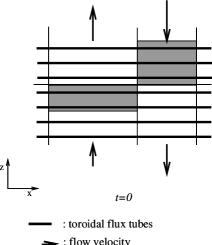
Figure 5.  : Turbulent pumping for a toroidal field.

2.7 Turbulent Pumping

The only inhomogeneous quantity is now $v^{2}$. As discussed in Sect. 2.4, in this case an asymmetry between up- and downflows is to be expected. In the case of weak inhomogeneity, implied by (51), we may use the linear relation $2F_{\rm kin}\sim-\rho lv_{t}d{v_{t}^{2}}/dz$. Comparing this with (52) we find $\Delta v=(v_{u}+v_{d})/2\simeq 2v\Delta f\sim-ldv/dz$ and $\Delta f=(f_{u}-f_{d})/2=\Delta v/2v\ll 1$. Then all expressions can be expanded into a series to first order in $\Delta f$; in this approximation $F_{\rm kin}/\rho\simeq 2v^{3}\Delta f$.

In the case of a poloidal field no turbulent pumping is expected to first order in $v\tau/H_{v^{2}}$, as the effect of the horizontal flow is again of higher order, and we are then back to the case of the density pumping of poloidal fields.

In the case of a toroidal field, with a manipulation similar to the previous cases (plus with an expansion in $\Delta f$), one can work out the result:

$${\cal E}_{y}=\langle v_{z}B_{x}-v_{x}B_{z}\rangle=-B_{0}\tau d_{z}{v^{2}}.$$ (59)

The pumping is directed downwards if the turbulent velocity decreases downwards. The interpretation of (one contribution to) the pumping is shown in Fig. 5: as a consequence of the continuity equation and of a downward directed kinetical energy flux, the downflows are faster and they process a larger amount of flux through the reference level than do the upflows, resulting in a net transport downwards. (Another contribution is due to the action of horizontal flow on tilted flux tube portions, an effect analoguous to the density pumping of toroidal fields.)

Turbulent pumping was discovered by ? (?), who christened the effect “turbulent diamagnetism”. This expression is sometimes still used, although it is in fact a misnomer. Real diamagnetism is a dynamical effect, resulting from the orienting effect of the magnetic field on the medium, while turbulent pumping is a purely kinematic phenomenon. There is not even a mathematical similarity between the two effects: diamagnetism exerts its influence through the $\mu$ permeability, i.e. it is formally more similar to turbulent diffusion than to the pumping that involves an advective-type term.

Another confusion related to turbulent pumping is that its expression is often quoted in the form

$$\gamma=\nabla\beta\sim\nabla(v^{2}\tau).$$ (60)

In the case when $\nabla\tau\neq 0$ this clearly differs from (40) and from (59). For 2D turbulence the first equality in (60) is indeed exact (?, ?) and it is also correct in 3D in order of magnitude. However, we should remember that the expression $\beta\sim\tau v^{2}$ is itself an order-of-magnitude formula only, so its differentiation will result in huge errors. The second (approximate) equality in (60) should therefore be used with caution.

Section 3 Higher Order and Nonlinear Effects

3.1 Geometrical and Topological Pumping

Geometrical pumping relies on the non-vanishing higher order correlation $\langle v_{x}\partial_{x}v_{z}\rangle$. The appearance of such a correlation implies that either the upflows or the downflows will have a mean horizontal divergence. The drag associated with these horizontal motions will then preferentially sweep the magnetic flux into the convergent component, which results in a net flux transport along the convergent component. For the sweeping effect to be significant in a correlation time $\tau$, a rather large (comparable to $v_{z}$) horizontal velocity component correlated with $\partial_{x}v_{z}$ is needed, which requires a strong inhomogeneity by virtue of the continuity equation (?, ?). Consequently, in turbulent flows this effect may only be important near a possible sharp boundary of the turbulent layer, and is therefore generally limited to low Reynolds number flows.

Topological pumping relies on a topological asymmetry of the up/downflows: in a horizontal cross-section of the layer, upflow areas may be connected, with isolated downflows or vice versa. A one-dimensional object like a field line will more easily be carried with the connected component. Of course, ultimately “what goes up must come down”, but, given sufficient time, magnetic diffusivity may be able to smooth out the resulting field into a mean field concentrated towards the direction of the connected flow. Again, the role of diffusivity implies that the effect will be more important for low magnetic Reynolds numbers.

These effects were much studied and became undeservedly widely known in the seventies and early eighties (?, ?, ?, ?, ?, ?, ?, ?) when it was hoped that they may offer a solution to the buoyancy problem pointed out by ? (?). The interest has dwindled after their unimportance was recognized in the high (magnetic) Reynolds number case. Recently, ? (?) used topological pumping as an argument against a supposed sharp lower boundary of the solar convective zone.

3.2 Negative Diffusivity and Small-Scale Dynamo

? (?) derived the expressions of $\hat{\alpha}$ and $\hat{\beta}$ for homogeneous turbulence in the fourth-order correlation approximation. One of their most interesting results is that the fourth-order correction to the diffusivity is negative, and it involves the helicity fluctuations. If the inhomogeneity of the field is strong, i.e. if $v_{\rm t}\tau\ll H_{B}$ does not hold, then this negative contribution may overcompensate the normal diffusivity.

A negative diffusivity implies that any small fluctuation will increase instead of being damped. In fact, no matter how large the overall scale of $\langle\mbox{\bf B}\rangle$ is, it may always develop infinitesimal small-scale fluctuations. The dominating negative term in $\beta$ for these small scales then means that these small fluctuations may reach large amplitudes before their growth is halted by nonlinear effects. This process does not influence the large-scale field, as the random fluctuations give no contribution to the net mean field; but it will influence $\langle|\mbox{\bf B}|\rangle$. In effect, the consequence of the negative diffusivity at small scales will be the appearance of a source term in the transport equation for $\langle|\mbox{\bf B}|\rangle$, beside the transport terms known from the transport equation of $\langle\mbox{\bf B}\rangle$ (cf. Sect. 3.4 above). Turbulence closure computations (?, ?, ?, ?, ?, ?) as well as numerical simulations (?, ?, ?, ?, ?, ?) indeed show this small-scale dynamo action. On their basis, in the high (magnetic) Reynolds number case the source term may be phenomenologically approximated by

$$\partial_{t}\langle|\mbox{\bf B}|\rangle=\langle|\mbox{\bf B}|\rangle[1-\langle|\mbox{\bf B}|\rangle/(f_{\rm m}B_{\rm eq})]v_{\rm t}/l,$$ (61)

where $f_{\rm m}\sim 0.1$ is the magnetic filling factor at the nonlinear saturation.

Physically, the small-scale dynamo relies on the existence of small-scale helicity fluctuations in the flow which increase the unsigned flux density by stretch-twist-fold type motions.

3.3 Magnetic Buoyancy

Although buoyancy was much studied in the case of active fields, its description in MFT was for a long time limited to the use of phenomenological sink terms in the mean induction equation. Recently however a major breakthrough was achieved by ? (?). In their SOCA treatment of the problem they recover the expected result $\gamma\propto\langle\mbox{\bf B}\rangle^{2}$ for weak fields. For fields closer to equipartition however, the buoyant loss is significantly reduced by the Lorentz force.

3.4 Density Self-Pumping and “Turbulent Buoyancy”

In Sect. 3 we have seen that anomalous pumping effects, e.g. density pumping, must rely on the anisotropy of the turbulence in a plane perpendicular to the pumping. The feedback of the magnetic field on the turbulence may itself induce such an anisotropy, thereby leading to the transport of the field. In particular, a horizontal anisotropy induced by a non-vertical magnetic field should lead to the vertical transport of the field. This problem was recently studied by ? (?). For strong fields they found a pumping downwards, in line with the expectation (the field should encourage turbulence in rolls around the field lines, which corresponds to the “poloidal” case depicted in Fig. 3). Surprisingly, however, for weak fields the pumping was found to be directed upwards. The origin of this curious phenomenon of “turbulent buoyancy”, as called by the authors, is unclear.

3.5 Other Effects

The above list is far from being exhaustive, even if we only regard the transport effects studied to date. As we go to higher orders, the number of new effects increases (although their importance will decrease, unless the inhomogeneity is very strong). Other effects are mentioned e.g. in ? (?), ? (?), ? (?).

An interesting but neglected aspect of the transport problem is the role of vorticity in the magnetic field transport. The association of vorticity with narrow downflows and its interaction with flux tubes (?, ?) suggests that a study of this problem would be worthwhile.

Section 4 Solar Applications

4.1 General Assessment and Convection Kinematics

Numerical simulations (?, ?) show that in a quasi-adiabatically stratified turbulent convective layer the $l$ correlation length is close to the $H_{P}$ pressure cale height. The scale heights of other mean quantities ($\rho$, $v_{\rm t}^{2}$, $\langle\mbox{\bf B}\rangle$ etc.) are usually greater than $H_{P}$, so in the deep solar convective zone the condition $l<H$ (though not $l\ll H$) is well satisfied, and the effects of first order in $l/H$, discussed in Sect. 2, may be expected to dominate in the mean field equation (with the notable exception of the small-scale dynamo source term in the equation for $\langle|\mbox{\bf B}|\rangle$, discussed in Sect. 3.2 above). On the other hand, near the boundaries of the convective zone (e.g. in the photosphere) we may have $l\gg H$ and higher order effects may become important.

But what is the relative importance of different first order effects? In particular, is there any region in the convective zone where the importance of dynamo terms is negligible, so that our discussion of “sterile” transport in a parity-invariant flow applies? As the expressions of the terms appearing in $\vec{\cal E}$ involved velocity correlations of different orders, in order to answer this question a model of the solar convective zone (SCZ) with a reliable description of convection kinematics is needed. Unfortunately, the available models of solar convection were developed either for the needs of stellar evolutionists, who only require an average stratification (and perhaps the extent of the overshoot) or for the needs of solar/stellar granulation observers, for whom nothing short of a full 3D numerical simulation is good enough. Dynamo theorists, with their medium-level requirements are not well served by contemporary convection theory. Nevertheless, the last decade has brought a number of advances in the difficult problem of convection kinematics. This field would be worth a review in itself, so here we only recall some results more directly relevant to our present problem.

The best available model of the SCZ that can be recommended for use by dynamo theorists is the model by Unno, Kondo and Xiong (?, ?, ?, ?); in what follows: the UKX model. This is a fully non-local model; its most important assumption is that third-order correlations are proportional to the gradients of second-order correlations; this is tantamount to the assumption of weak inhomogeneity. More restrictive from the point of view of magnetic field transport theory is the assumption of a constant radial anisotropy ($\langle v_{r}^{2}\rangle=2\langle v_{\theta}^{2}\rangle=2\langle v_{\phi}^{2}\rangle$). As we have seen in Sect. 2, the anisotropy of turbulence plays an important role in the transport. ? (?) computed the anisotropy of low Prandtl number turbulent convection in the homogeneous (Boussinesq) case. Inhomogeneity may however significantly modify the anisotropy. In a later work, ? (?) evaluated the full anisotropy under the (invalid) assumption that inhomogeneity only influences the part of horizontal velocity that is correlated with the radial motions. In a complementary work, ? (?) computed the full anisotropy caused by inhomogeneity in the case of quasi-isotropic original turbulence; this latter work also incorporates the effect of rotation. Although a complete solution of the anisotropy problem is still not around, the available results suggest that the anisotropy (both radial and horizontal) in the SCZ is significant, but not extreme.

Figure 6.  : Characteristic velocites as functions of depth in the solar convective zone. Note that only an the upper limit on $\alpha$ compatible with the given kinetic energy and an upper limit on the density pumping velocity corresponding to the unlikely case of maximal anisotropy (meridional rolls) are displayed.

Fig. 6 shows the characteristic velocities corresponding to different terms in the mean field transport equation as functions of depth in the SCZ. The relative magnitudes of the velocities characterize the relative importance of these terms. It is apparent that with the exception of the bottom of the SCZ the $\alpha$ term is by orders of magnitude smaller than the transport terms. The characteristic velocity difference due to the shear by differential rotation (not shown) has a similar behaviour. This implies that with the exception of the bottom of the SCZ the dynamo terms are indeed negligible in comparison with the transport terms: in a simplistic treatment the solar dynamo may be split into a thin generation layer at bottom and a deep turbulent zone above; the distribution of the field generated in the dynamo layer will be determined by a dynamical equilibrium of turbulent transport processes in the convective zone. Of course we should keep in mind that part of the magnetic field intruding into the convective zone from the dynamo layer below will be in active form (e.g. the thick flux loops giving rise to AR). The decay of such thick active tubes may act as a local source of passive fields in the convective zone. The amplitude of this active source may be determined from observations of AR decay at the surface; but in deeper layers it presents a large uncertainty in our discussions of passive field transport.

As mentioned above, higher order effects may come into play near the boundaries of the SCZ. This is likely to be the case in the photosphere where $l\gg H_{P}$, but unfortunately very little is known about flux transport in these circumstances. In an ongoing effort (?, ?) the observed photospheric height-dependence of $\langle|\mbox{\bf B}|\rangle$ is compared to vertical transport equilibrium models (as yet only including first order effects). In agreement with observations, these models indicate that $\langle|\mbox{\bf B}|\rangle\mathrel{\mathchoice{\vbox{\offinterlineskip\halign{\hfil$\displaystyle#$\hfil\cr<\cr\sim\cr}}}{\vbox{\offinterlineskip\halign{\hfil$\textstyle#$\hfil\cr<\cr\sim\cr}}}{\vbox{\offinterlineskip\halign{\hfil$\scriptstyle#$\hfil\cr<\cr\sim\cr}}}{\vbox{\offinterlineskip\halign{\hfil$\scriptscriptstyle#$\hfil\cr<\cr\sim\cr}}}}1$ mT at the top of the photosphere. Whether such a low magnetic energy density is sufficient to explain the observed basal chromospheric Ca II K flux, as proposed by ? (?), remains to be seen.

The lower boundary of the SCZ presents an even more vexing problem. Phenomenological non-local mixing-length models traditionally predict a very sharp lower boundary with $v_{\rm t}^{2}$ suddenly dropping to zero in a thin layer. As pointed out by ? (?), in this case the extremely low velocity scale height should lead to strong geometrical and topological pumping. The flow topology in this layer is expected to be $d$-type in the notations of ? (?), so all flux would be removed upwards from the dynamo layer. This contradiction seems to make it unlikely that the SCZ has a sharp lower boundary. In the models, the sharp bottom is a consequence of the a priori assumption of a good correlation between velocity and temperature fluctuations which is not granted in the overshooting layer. Indeed, the more realistic UKX model shows a much more gradual decrease of $v_{\rm t}^{2}$ at the lower boundary with $H_{v^{2}_{\rm t}}\sim H_{P}$. This result agrees with numerical experiments (?, ?, Brandenburg, private comm.) and helioseismological constraints (?, ?). The problem is further complicated by the influence of magnetic fields and differential rotation on the structure of this important layer of the Sun.

4.2 Vertical transport

Fig. 6 shows that the most important vertical transport effects are turbulent diffusion and turbulent pumping. The vertical distribution of passive magnetic flux in the SCZ should therefore be determined by a dynamical equilibrium of these processes, possibly influenced by density pumping and/or an active source. As $v_{\rm t}$ has a maximum at a shallow depth of 200 km in the UKX model, we may expect that the downwards directed turbulent pumping will “press” the field down to the bottom of the convective zone as far as turbulent diffusion, trying to “smooth out” the distribution, will allow. If for simplicity we regard a 1D plane parallel model with $\langle B_{y}\rangle=0$, the only non-trivial component of the transport equation (35)–(36) is

$$0=d_{z}(\beta_{zz}d_{z}\langle B_{x}\rangle)+d_{z}[(\gamma_{z}+\tilde{\gamma}_{z})B_{x}],$$ (62)

with coefficients given by (39)–(41).

The vertical passive magnetic flux transport through the SCZ in a formulation similar to (62) was apparently first considered by ? (?). By analogy with the density pumping of a poloidal magnetic field in 2D convection he proposed that the vertical transport is determined by a strong density pumping downwards. Soon thereafter, ? (?) showed that vertical density pumping will vanish for horizontally isotropic turbulence, and ? (?) stressed the importance of turbulent pumping in the vertical transport. The confusion concerning the correct expression of turbulent pumping, discussed above (end of Sect. 2.7), however led many to the false belief that turbulent pumping is negligible in the SCZ. As a consequence of this, density pumping made a comeback in the first quantitative study of the problem by ? (?). The heuristic transport equation used in this work was in effect equivalent to (62) containing only a (downwards) density pumping term and turbulent diffusion. An approximate analytic solution was also presented. Kichatinov’s (?) study of the density pumping was applied to the SCZ by ? (?).

The somewhat speculative early models came into a different light with the new observational results summarized in Sect. 1.2 above. In order to see what these empirical constraints imply for the vertical distribution of passive magnetic flux, ? (?) solved equation (62) using boundary conditions taken from the observations and including turbulent pumping and turbulent diffusion, but neglecting the contribution due to the third and fourth terms in (38). ? (?) extended this work by including the neglected terms and the effects of sphericity (in an approximation that still preserved the mathemtical one-dimensionality of the problem). Equation (62) can be integrated to yield

$$\beta_{zz}d_{z}\langle B_{x}\rangle+(\gamma_{z}+\tilde{\gamma}_{z})\langle B_{x}\rangle=-L_{\rm m},$$ (63)

where the $L_{\rm m}$ integration constant is the net flux loss from the Sun and it must obviously lie between 0 and $v_{\rm t,s}\langle B_{x}\rangle_{\rm s}$ (‘s’ index refers to values near the surface, ‘b’ to those at the bottom of the SCZ). Observations show that outside unipolar network areas $\langle B_{z}\rangle$ is typically order of 0.01–0.1 mT; this may also be applied to $B_{x}$ at some depth below the surface, assuming that averaging over the solar surface the ratio $|\langle B_{x}\rangle|/|\langle B_{z}\rangle|\sim 1$. Figure 7 (left) shows the numerical solutions of the transport equation with different boundary conditions. It is apparent that the flux density increases by several orders of magnitude to the bottom of the SCZ, confirming our expectation. Turbulent pumping therefore has the important role of “helping” the dynamo by sweeping the escaping flux back to the dynamo layer very effectively. It is also apparent that a relatively low flux density of $\sim 100$ mT at the bottom will lead to a surface field comparable to that observed. Indeed, it is quite possible that all the net flux observed on the surface originates from passive fields in the dynamo layer by direct diffusion. On the other hand, we must remember that active source terms (neglected in (62)) may also be a significant source of net field. The observed rate of flux emergence in AR is too low to significantly modify the distribution (dynamical equilibrium is reached on a timescale $\sim 20$ days, comparable to the turbulent correlation time in the deep SCZ!) but AR may still be an important source of flux on a long term. In this latter case, the flux input by AR would be reprocessed by turbulent transport through the whole convective zone and would reappear again and again in a passive form. Finally, the possibility cannot be excluded that a much stronger active source operates in the deep SCZ in the form of a large number of “failed active regions” (?, ?): rising flux loops decaying before they could make it to the surface.

Figure 7.  : Mean net flux density (left) and mean unsigned flux density (right) as functions of depth in the SCZ. Short dashes denote $B_{\rm eq}$ (left) and $f_{\rm m}B_{\rm eq}$ (right); other curves are solutions with different boundary conditions (see ?, ?, for a detailed legend).

An equation similar to (62), with the added source term (61) should determine the equilibrium distribution of the unsigned flux density $\langle|B_{x}|\rangle$. The integration of this equation (?, ?, ?, ?) yields the results shown in Fig. 7 (right). Note the weak dependence on the boundary conditions applied and note that the surface value of the unsigned flux density (2.5–7.5 mT) is not a boundary condition here but an output in nice agreement with the observations of ? (?). In fact the results show that even the resolved unsigned passive flux density of 0.5–1 mT (cf. Sect. 1.2) is incompatible with a transport equation without source term; this can be regarded as indirect evidence for the operation of a small-scale dynamo mechanism in the Sun.

4.3 Horizontal and 2D Transport

The idea that horizontal transport of passive fields by meridional circulation and/or turbulent diffusion may have an important role in the solar dynamo goes back to ? (?) and ? (?) who proposed that the poleward drift of $f$-polarity background fields at high latitudes is due to these effects. These two effects were combined into a single model by ? (?) and further developed until a detailed comparison with synoptic magnetic maps yielded very positive results (?, ?). Despite their success in interpreting the synoptic maps, these 1D horizontal transport models seem to be in conflict with the results of ? (?), discussed in Sect. 1.2, which imply that the large-scale field pattern should be refreshed on a timescale of 3–30 days. Indeed, as we have seen, the vertical transport models yield a vertical transport timescale of $\sim 20$ days: over this time, the flux is vertically processed through the whole of the SCZ. The contradiction may disappear if we assume that the horizontal transport processes regarded by ? (?) act throughout the whole SCZ. This would give a natural explanation for the remarkably low diffusivity (600 km²/s, much lower than $\tau v_{\rm t}^{2}\sim 10^{4}$ km²/s for the supergranulation) required by the comparison with the synoptic maps: this is about the value of $\tau v_{\rm t}^{2}$ in the deep SCZ.

In order to check whether the results of the horizontal diffusion models remain valid, detailed 2D (horizontal+vertical) models of magnetic flux transport are clearly needed. A first step in this direction was made by ? (?) where the vertical dimension was included by a kind of vertical truncation of the equations. In Budapest we are presently working on a fully 2D model of the field transport; this model involves the numerical solution of equations (24–26) with proper boundary conditions. Preliminary results from a fast implicit integration of a simplified, approximate form of the poloidal equation on a uniform $200\times 1000$ grid show that the behaviour of the solution qualitatively agrees with the expectation, i.e. turbulent pumping presses down the field.

A potential use of 2D transport models is to forge a link between the field distribution seen on the surface (as represented by synoptic maps or spherical harmonic expansions) and the field in the dynamo layer, thereby imposing an observational constraint on dynamo models. But the transport may also turn out to have a more fundamental role than this. If the 1D results of ? (?) are confirmed in 2D, then the “poleward branch” of the butterfly diagram is fully due to field transport effects, instead of being a dynamo wave. In fact, ? (?) has proposed that transport effects may interpret both branches of the butterfly diagram: the horizontal density pumping should transport the toroidal field equatorwards, the poloidal field polewards. Clearly, the full role of flux transport mechanisms in the dynamo can only be judged after full 2D transport models become available.

Acknowledgements. I thank Rob Rutten for inviting me to the workshop. I am grateful to NATO and to the Soros Foundation for their financial support.

References

- Arter (1983a) Arter, W.: 1983a, J. Fluid Mech. 132, 25
- Arter (1983b) Arter, W.: 1983b, in J. O. Stenflo (Ed.), Solar and Stellar Magnetic Fields: Origins and Coronal Effects, Proc. IAU Symp. 102, Reidel, Dordrecht, p. 243
- Arter (1985) Arter, W.: 1985, Geophys. Astrophys. Fluid Dyn. 31, 311
- Babcock (1961) Babcock, H. W.: 1961, ApJ 133, 572
- Cattaneo et al. (1988) Cattaneo, F., Hughes, D. W., and Proctor, M. R. E.: 1988, Geophys. Astrophys. Fluid Dyn. 41, 335
- Cattaneo and Vainshtein (1991) Cattaneo, F. and Vainshtein, S. I.: 1991, ApJ 376, L21
- Chan and Sofia (1987) Chan, K. L. and Sofia, S.: 1987, Sci 235, 465
- Csada (1951) Csada, I. K.: 1951, Acta Phys. Hung. 1, 235
- De Young (1980) De Young, D. S.: 1980, ApJ 241, 81
- Drobyshevski (1977) Drobyshevski, E. M.: 1977, Ap&SS 46, 41
- Drobyshevski et al. (1980) Drobyshevski, E. M., Kolesnikova, E. N., and Yuferev, V. S.: 1980, J. Fluid Mech. 101, 65
- Drobyshevski et al. (1974) Drobyshevski, E. M., Yuferev, V. S., and Moffatt, H. K.: 1974, J. Fluid Mech. 65, 33
- Durney et al. (1993) Durney, B. R., De Young, D. S., and Roxburgh, I. W.: 1993, Sol. Phys. 145, 207
- Faurobert-Scholl (1993) Faurobert-Scholl, M.: 1993, A&A 268, 765
- Faurobert-Scholl et al. (1994) Faurobert-Scholl M., Feautrier N., Machefert F., Petrovay K., and Spielfiedel A.: 1994, A&A 298, 289
- Howard and Stenflo (1972) Howard, R. and Stenflo, J. O.: 1972, Sol. Phys. 22, 402
- Hoyng (1994) Hoyng, P.: 1994, in C. J. Schrijver and R. J. Rutten (Eds.), Solar Surface Magnetism, NATO ASI Series, Kluwer, Dordrecht
- Keller (1994) Keller, C. U.: 1994, in C. J. Schrijver and R. J. Rutten (Eds.), Solar Surface Magnetism, NATO ASI Series, Kluwer, Dordrecht
- Kichatinov (1991) Kichatinov, L. L.: 1991, A&A 243, 483
- Kichatinov and Pipin (1993) Kichatinov, L. L. and Pipin, V. V.: 1993, A&A 274, 647
- Kichatinov and Rüdiger (1992) Kichatinov, L. L. and Rüdiger, G.: 1992, A&A 260, 494
- Kichatinov and Rüdiger (1993) Kichatinov, L. L. and Rüdiger, G.: 1993, A&A 276, 96
- Krause (1978) Krause, F.: 1978, Publ. Astron. Inst. Czechoslov. 54, 41
- Krivodubskij and Kichatinov (1991) Krivodubskij, V. N. and Kichatinov, L. L.: 1991, in I. Tuominen, D. Moss, and G. Rüdiger (Eds.), The Sun and Cool Stars: Activity, Magnetism, Dynamos, ProcİAU Coll. 130, Springer, Berlin, p. 190
- Leighton (1964) Leighton, R. B.: 1964, ApJ 140, 1547
- Leorat et al. (1981) Leorat, J., Pouquet, A., and Frisch, U.: 1981, J. Fluid Mech. 104, 419
- Livingston and Harvey (1971) Livingston, W. and Harvey, J.: 1971, in R. Howard (Ed.), Solar Magnetic Fields, Proc. IAU Symp. 43, Reidel, Dordrecht, p. 51
- Ludwig (1994) Ludwig, H.-G.: 1994, in M. Schüssler (Ed.), Solar Magnetic Fields, Proc. Freiburg Internat. Conf., Cambridge UP
- Martin (1990) Martin, S. F.: 1990, in J. O. Stenflo (Ed.), Solar Photosphere: Structure, Convection and Magnetic Fields, Proc. IAU Symp. 138, Kluwer, Dordrecht, p. 129
- Martin (1994) Martin, S. F.: 1994, in C. J. Schrijver and R. J. Rutten (Eds.), Solar Surface Magnetism, NATO ASI Series, Kluwer, Dordrecht
- Meneguzzi et al. (1981) Meneguzzi, M., Frisch, U., and Pouquet, A.: 1981, Phys. Rev. Letters 47, 1060
- Meneguzzi and Pouquet (1989) Meneguzzi, M. and Pouquet, A.: 1989, J. Fluid Mech. 205, 897
- Moffatt (1983) Moffatt, H. K.: 1983, Rep. Prog. Phys. 46, 621
- Monteiro et al. (1994) Monteiro, M. J. P. F. G., Christensen-Dalsgaard, J., and Thompson, M. J.: 1994, A&A in press
- Murray (1992a) Murray, N.: 1992a, Sol. Phys. 138, 419
- Murray (1992b) Murray, N.: 1992b, ApJ 401, 386
- Nicklaus and Stix (1988) Nicklaus, B. and Stix, M.: 1988, Geophys. Astrophys. Fluid Dyn. 43, 149
- Nordlund et al. (1992) Nordlund, Å., Brandenburg, A., Jennings, R. L., Rieutord, M., Ruokolainen, J., Stein, R. F., and Tuominen, I.: 1992, ApJ 392, 647
- Parker (1955) Parker, E. N.: 1955, ApJ 122, 293
- Parker (1975) Parker, E. N.: 1975, ApJ 198, 205
- Parker (1979) Parker, E. N.: 1979, Cosmical Magnetic Fields, Clarendon, Oxford
- Parker (1982) Parker, E. N.: 1982, ApJ 256, 302
- Petrovay (1990) Petrovay, K.: 1990, ApJ 362, 722
- Petrovay (1991) Petrovay, K.: 1991, in I. Tuominen, D. Moss, and G. Rüdiger (Eds.), The Sun and Cool Stars: Activity, Magnetism, Dynamos, Proc. IAU Coll. 130, Springer, Berlin, p. 67
- Petrovay (1992) Petrovay, K.: 1992, Geophys. Astrophys. Fluid Dyn. 65, 183
- Petrovay (1993) Petrovay, K.: 1993, in W. Weiss and A. Baglin (Eds.), Inside the Stars, Proc. IAU Coll. 137, Conf. Series Astron. Soc. Pacif. 40, 293
- Petrovay (1994) Petrovay, K.: 1994, in M. Schüssler (Ed.), Solar Magnetic Fields, Proc. Freiburg Internat. Conf., Cambridge UP, p. 146
- Petrovay and Szakály (1993) Petrovay, K. and Szakály, G.: 1993, A&A 274, 543
- Rädler (1976) Rädler, K.-H.: 1976, in V. Bumba and J. Kleczek (Eds.), Basic Mechanisms of Solar Activity, Proc. IAU Symp. 71, Reidel, Dordrecht, p. 323
- Rädler (1980) Rädler, K.-H.: 1980, Astron. Nachr. 301, 101
- Schüssler (1984) Schüssler, M.: 1984, in T. D. Guyenne and J. J. Hunt (Eds.), The Hydromagnetics of the Sun, Proc. 4th Eur. Meeting on Sol. Phys., ESA, p. 67
- Sheeley (1966) Sheeley, N. R.: 1966, ApJ 144, 723
- Sheeley et al. (1985) Sheeley, N. R., DeVore, C. R., and Boris, J. P.: 1985, Sol. Phys 98, 219
- Spruit et al. (1987) Spruit, H. C., Title, A. M., and van Ballegooijen, A. A.: 1987, Sol. Phys. 110, 115
- Steenbeck et al. (1966) Steenbeck, M., Krause, F., and Rädler, K.-H.: 1966, Zs. Naturforschung A 21, 369
- Stenflo (1973) Stenflo, J. O.: 1973, Sol. Phys. 32, 41
- Stenflo (1982) Stenflo, J. O.: 1982, Sol. Phys. 80, 209
- Stenflo (1987) Stenflo, J. O.: 1987, Sol. Phys. 114, 1
- Stenflo (1992) Stenflo, J. O.: 1992, in K. L. Harvey (Ed.), The Solar Cycle, NSO/Sacramento Peak 12th Summer Workshop, Astron. Soc. Pacif. Conf. Proc., p. 83
- Stenflo and Lindegren (1977) Stenflo, J. O. and Lindegren, L.: 1977, A&A 59, 367
- Sweet (1950) Sweet, P. A.: 1950, MNRAS 110, 69
- Unno and Kondo (1989) Unno, W. and Kondo, M.: 1989, PASJ 41, 197
- Unno et al. (1985) Unno, W., Kondo, M., and Xiong, D.-R.: 1985, PASJ 37, 235
- Vainshtein (1978) Vainshtein, S. I.: 1978, Magn. Gidrodin. 2, 67
- Wang et al. (1989) Wang, Y.-M., Nash, A. G., and Sheeley, N. R.: 1989, ApJ 347, 529
- Wang et al. (1991) Wang, Y.-M., Sheeley, N. R., and Nash, A. G.: 1991, ApJ 383, 431
- Weiss (1964) Weiss, N. O.: 1964, Phil. Trans. Roy. Soc. A 256, 99
- Zeldovich (1957) Zeldovich, Y. B.: 1957, Sov. Phys-JETP 4, 460
- Zirin (1986) Zirin, H.: 1986, Aust. J. Phys. 38, 961
- Zwaan (1994) Zwaan, C.: 1994, in M. Schüssler (Ed.), Solar Magnetic Fields, Proc. Freiburg Internat. Conf., Cambridge UP, p.