Abstract

A model for homogeneous anisotropic incompressible turbulence is proposed. The model generalizes the GISS model of homogeneous isotropic turbulence; the generalization involves the solution of the GISS equations along a set of integration paths in wavenumber (k-) space. In order to make the problem tractable, these integration paths (“cascade lines”) must be chosen in such a way that the behaviour of the energy spectral function along different cascade lines should be reasonably similar. In practice this is realized by defining the cascade lines as the streamlines of a cascade flow; in the simplest case the source of this flow may be identified with the source function of the turbulence. Owing to the different approximations involved, the resulting energy spectral function is not exact but is expected to give good approximative values for the bulk quantities characterising the turbulent medium, and for the measure of the anisotropy itself in particular.

The model is then applied to the case of low Prandtl number thermal convection. The energy spectral function and the bulk quantities characterizing the flow are derived for different values of the parameter $S=\mbox{Ra}\,\sigma$. The most important new finding is that unlike the anisotropy of the most unstable mode in linear stability analysis the anisotropy of the turbulence does not grow indefinitely with increasing $S$ but it rather saturates to a relatively moderate finite asymptotic value. Anisotropy, convection, turbulence.

Section 1 INTRODUCTION

In recent years it has become clear that a better understanding of the anisotropy of turbulence in stellar convective zones is important for several reasons. It is now widely believed that the anisotropy of turbulence plays a key role in governing the transport of angular momentum in the convective zones of stars and therefore in determining their differential rotation (Rüdiger, 1989). More accurate knowledge of the anisotropy could therefore constrain the theories of differential rotation, which at present involve a large number of free parameters. Furthermore, it is possible to show (Petrovay, 1990) that the intriguing morphological properties of solar and stellar convection found in recent numerical simulations (Stein and Nordlund, 1989, Nordlund and Dravins, 1990) can be predicted on the basis of sufficiently general convection theories if the anisotropy is known. From its influence on differential rotation and on the morphology of convection it follows that the anisotropy of turbulence is important in understanding the dynamo mechanism (Brandenburg et al. , 1991, Petrovay, 1991). Finally, some current theories of stellar convection (e.  g.  Xiong, 1980) rely on the assumption that the anisotropy of turbulence remains moderate throughout the convective layer, while other formalisms (Canuto 1989, 1990) include the anisotropy as a free parameter to be specified. All this suggests that a method to compute the anisotropy of turbulence that is simple enough to be applicable in practice while it still retains the essential physical ingredients of the problem could be very useful in several astrophysical areas.

It seems to be plausible to treat homogeneous anisotropic turbulence as a first step. Despite the fact that homogeneous anisotropic turbulence is “to some extent a non-problem” (Leslie 1973), in the sense that any process generating (anisotropic) turbulence relies on the presence of an inhomogeneity on the large scales while the turbulence becomes isotropic on the small scales, it has been widely recognized that the study of this subject is of high importance for several reasons. First, it is expected that with increasing $k$ wavenumber the turbulence tends to homogeneity faster than to isotropy (Leslie 1973), so there exists a wavenumber-regime where the model applies. Secondly, in certain flows (e. g.  in grid turbulence sufficiently far from the grid) the homogeneous anisotropic approximation may be valid even on the scale of the energy-containing eddies. Thirdly, and perhaps most importantly, the study of homogeneous and anisotropic turbulence may be an important intermediate step towards the fully general case of inhomogeneous anisotropic turbulence.

As efforts to tackle the problem of anisotropic turbulence on the basis of two-point closure models like the DIA did not bear much fruit owing to the intimidating complexity of the equations, Canuto et al.  (1990) propose that, to begin with, simpler heuristic models should be used, followed by the construction of more complex models (in analogy with the historical development of the theory of homogeneous isotropic turbulence).

Figure 1.  : The anisotropy of the “typical” (T) and the strongest (S) mode may be similar or totally different, depending on how sharply peaked the spectral function is.

The measure of anisotropy is usually characterised by quantities like

$$x=\frac{l_{z}^{2}}{l_{x}^{2}+l_{y}^{2}}$$ (1)

or

$$s=\frac{\overline{v_{x}^{2}}}{\overline{v_{z}^{2}}}$$ (2)

where $l_{x}$, $l_{y}$, $l_{z}$ are “characteristic scales” of the turbulence (e. g.  macroscales or correlation lengths) in different directions, v is the turbulent velocity and $z$ is a preferred direction (e. g.  due to gravity). In contemporary practice values of these quantities are often “guessed” on the basis of their values for the most unstable mode in linear stability analysis. Turbulent values for the diffusivities are sometimes used in the analysis as an attempt to take the nonlinear interaction of modes into account. It is however rather uncertain whether the anisotropy computed in this way represents the anisotropy of the turbulence correctly, not only because nonlinear mode interactions may be expected to distort the shape of the spectrum shifting the maximum, but also because quantities like (1) or (2) are defined as averages over all wavenumbers, weighted e. g.  by

$$\Phi_{ij}(\mbox{\bf k})=\frac{1}{(2\pi)^{3}}\int\exp(-i\mbox{\bf k}\underline{\xi})\overline{v_{i}(\mbox{\bf r})v_{j}(\mbox{\bf r}+\underline{\xi})}\,d^{3}\xi,$$ (3)

the velocity covariance spectral function (or its trace $F\equiv\Phi_{ii}$), and not as values for the single mode corresponding to the maximum of $F(\mbox{\bf k})$. The difference is highlighted in Figure 1 (for the sake of clarity in one dimension). Depending on how sharply peaked $F(\mbox{\bf k})$ is, the “typical” k value may be similar to or totally different from the location of the maximum of $F(\mbox{\bf k})$.

In fact, for the case of low Prandtl number convective turbulence in numerical experiments the value of the $s$ parameter defined in (2) is found to be very nearly constant at a moderate value of $s\simeq 0.37$ for a range of the

$$S=\mbox{Ra}\,\sigma=\frac{g\delta\beta D^{4}}{\chi^{2}}$$ (4)

parameter covering several orders of magnitude (Chan and Sofia, 1989). (Ra is the Rayleigh number, $\sigma$ the Prandtl number, $g$ the gravity acceleration, $\delta$ the volume expansion coefficient, $\beta$ the superadiabatic temperature gradient, $\chi$ the thermodiffusion coefficient, $D$ the layer depth, usually identified with the $H_{P}$ pressure scale height.) This is in contrast with the anisotropy of the most unstable mode in linear stability analysis which grows indefinitely with increasing $S$ (Canuto, 1990). On the other hand, Canuto (1990) has shown that if molecular diffusivities are replaced by turbulent ones in the linear analysis, the anisotropy of the most unstable mode, though still quite high and slowly increasing with $S$, will be seriously reduced. This was the first theoretical result indicating that nonlinear interactions of modes have the potential to limit the anisotropy of turbulence.

The present paper proposes a method to derive the measure of the anisotropy as well as other bulk quantities in a consistent (though approximate) way. Section 2 contains the general description of the method. This model is then applied to the astrophysically relevant case of low Prandtl number convective turbulence in Section 3. The results, summarized in Section 4, agree with the above mentioned numerical simulations. Section 5 concludes the paper.

Section 2 THE MODEL

2.1 General description of the model

The model presented below is a generalization of the GISS model developed by Canuto, Goldman and Chasnov (1987, hereafter CGC). The GISS model is a single-point closure scheme belonging to the class of “turbulent viscosity approach” models; it has been shown to compare well with experiments and DIA results (see CGC).

We suppose that $\Phi_{ij}(\mbox{\bf k})$ is a “smooth” function, i. e.  that the spectrum of the allowed modes is not discrete. In cases of astrophysical interest, for which this model was primarily developed, this is often a reasonable approximation as the studied turbulent regions here form parts of much larger systems (e. g.  stars) and so the eigenmodes populate the k-space densely enough. The assumption may also be reasonably valid in some laboratory experiments (e. g.  grid turbulence). However, for systems with a discrete and sparsely populated mode spectrum the present approach cannot be applied.

In its principal axis frame the velocity covariance spectral function takes the form

$$\hat{\Phi}=\left(\begin{array}[]{ccc}\Phi_{1}&0&0\\ 0&\Phi_{2}&0\\ 0&0&\Phi_{3}\end{array}\right).$$ (5)

For each $\Phi_{i}(\mbox{\bf k})$ component we have an $n_{S,i}(\mbox{\bf k})$ source function or growth rate, supposed to be known from the linear stability analysis. (The dissipation rate is also supposed to be built into $n_{S,i}$.) So we can form an $\hat{n}_{S}$ source tensor function in such a way that in the principal axis frame of $\hat{\Phi}$ the form of $\hat{n}_{S}$ is

$$\hat{n}_{S}=\left(\begin{array}[]{ccc}n_{S,1}&0&0\\ 0&n_{S,2}&0\\ 0&0&n_{S,3}\end{array}\right).$$ (6)

The total energy input per unit time into a given k mode is then $\hat{n}_{S}(\mbox{\bf k}):\hat{\Phi}(\mbox{\bf k})$. ($\hat{A}:\hat{B}\equiv A_{ij}B_{ij}$.)

The basic equation of the model expresses the equality of the energy fed into a given $\cal V$ volume of the k-space with the energy transferred away from that volume:

$$\int_{\cal V}\hat{n}_{S}({\mbox{\bf k}}^{\prime}):\hat{\Phi}({\mbox{\bf k}}^{\prime})\,d^{3}k^{\prime}=\int_{\cal V}\,d^{3}k^{\prime}\int_{\overline{\cal V}}T({\mbox{\bf k}}^{\prime},{\mbox{\bf k}}^{{}^{\prime\prime}})\,d^{3}k^{{}^{\prime\prime}},$$ (7)

$\overline{\cal V}$ being the complement of $\cal V$. The $T({\mbox{\bf k}}^{\prime},{\mbox{\bf k}}^{{}^{\prime\prime}})$ transfer term is to be determined by the closure. In the turbulent viscosity approach the r.  h.  s.  of equation (6) is taken to be the product of the total vorticity of modes in $\cal V$ with the turbulent viscosity.

In the case of isotropy equation (7) for a continuous manifold of spheres centered on the origin of the coordinate frame uniquely determines $\hat{\Phi}$, once $\hat{\alpha}\equiv\hat{\Phi}/F$ is specified. In the case of anisotropy, however, we need several (in general three) such intersecting manifolds of surfaces. Equivalently, one may take a continuous manifold of curves originating from a common $P$ starting point and covering the k-space. This manifold defines a “curvilinear polar coordinate frame” with coordinates $\kappa$, $\theta_{C}$, $\phi_{C}$ ($\kappa$ is the length along each curve measured from $P$, the $\theta_{C}$ and $\phi_{C}$ “angles” effectively index the curves). Now in equation (7) we may choose for $\cal V$ a “curvilinear cone” with angle $\Delta\Omega_{C}$ centered around the $0<\kappa^{\prime}<\kappa$ stretch of the $(\theta_{C},\phi_{C})$ curve. Taking the $\Delta\Omega_{C}\rightarrow 0$ limit and using the notation $k_{c}^{2}$ as defined by

$$d^{3}k=k_{c}^{2}\,d\kappa\,d\Omega_{C}$$ (8)

we get

$$\int_{0}^{\kappa}\hat{n}_{S}(\kappa^{\prime},\theta_{C},\phi_{C}):\hat{\Phi}(\kappa^{\prime},\theta_{C},\phi_{C})k_{c}^{2}(\kappa^{\prime},\theta_{C},\phi_{C})\,d\kappa^{\prime}=y(\kappa,\theta_{C},\phi_{C})\nu_{t}(\kappa,\theta_{C},\phi_{C})$$ (9)

where

$$y(\kappa,\theta_{C},\phi_{C})=\int_{0}^{\kappa}F(\kappa^{\prime},\theta_{C},\phi_{C})k^{2}(\kappa^{\prime},\theta_{C},\phi_{C})k_{c}^{2}(\kappa^{\prime},\theta_{C},\phi_{C})\,d\kappa^{\prime}$$ (10)

is the total vorticity along the $(0,\kappa)$ stretch of the curve.

According to the turbulent viscosity concept $\nu_{t}$ can be written in the form of an integral of independent contributions. On a purely dimensional basis

$$\nu_{t}(\kappa,\theta_{C},\phi_{C})=\int_{\overline{\cal V}(\kappa,\theta_{C},\phi_{C})}\frac{F(\mbox{\bf k}^{{}^{\prime\prime}})}{n_{c}(\mbox{\bf k}^{{}^{\prime\prime}})}\,d^{3}k^{{}^{\prime\prime}},\hfill(11)$$ (11)

$n_{c}^{-1}$ being a characteristic timescale of the turbulence. The GISS model closure is

$$\gamma n_{c}=k^{2}\nu_{t}$$ (12)

($\gamma=(2/3\mbox{Ko})^{3}$ where Ko is the Kolmogorov constant).

Equation (11) shows that in order to solve the system of equations along a given path, the value of $F$ must be known along all the other paths. How can we avoid this awkward recursion?

Suppose that our choice of the integration paths is so fortunate that the behaviour of $F(\kappa)=F(\kappa,\theta_{C},\phi_{C})$ is very similar (or even identical) for all $(\theta_{C},\phi_{C})$ paths. In the case of this “fortunate” choice we will call the paths cascade lines. Equation (11) can now be written as

$$\nu_{t}(\kappa,\theta_{C},\phi_{C})=4\pi\int_{\kappa}^{\infty}k_{c}^{2}(\kappa^{{}^{\prime\prime}},\theta_{C},\phi_{C})\frac{F(\kappa^{{}^{\prime\prime}},\theta_{C},\phi_{C})}{n_{c}(\kappa^{{}^{\prime\prime}},\theta_{C},\phi_{C})}\,d\kappa^{{}^{\prime\prime}},$$ (13)

i. e.  the integration over the angles could be replaced by a $4\pi$ factor and the recursion has disappeared. The method of finding the cascade lines (i. e. such a fortunate choice of paths) will be discussed in the next subsection.

Now the equations (9), (10), (12) and (13) can be transformed into a more convenient form, following the treatment in CGC with slight modifications.

Differentiating (9) with respect to $\kappa$ and using the notation $\hat{\alpha}=\hat{\Phi}/F$ we get

$$(\hat{n}_{S}:\hat{\alpha})+4\pi yn_{c}^{-1}=\nu_{t}k^{2}.$$ (14)

From this

$$2\gamma n_{c}=(\hat{n}_{S}:\hat{\alpha})+\left[(\hat{n}_{S}:\hat{\alpha})^{2}+16\pi\gamma y\right]^{1/2}.$$ (15)

Still following CGC we introduce

$$V=4\pi y+{\textstyle\frac{1}{2}}\gamma n_{c}^{2}.\hfill(16)$$ (16)

With this, equation (15) becomes

$$\gamma n_{c}={\textstyle\frac{1}{3}}(\hat{n}_{S}:\hat{\alpha})+\left[{\textstyle\frac{1}{9}}(\hat{n}_{S}:\hat{\alpha})^{2}+{\textstyle\frac{2}{3}}\gamma V\right]^{1/2}.$$ (17)

Now differentiating (16) and using the closure (12)

$$\frac{\partial V}{\partial\kappa}=\gamma n_{c}^{2}\frac{1}{k^{2}}\frac{\partial k^{2}}{\partial\kappa}.$$ (18)

(Partial derivatives are taken with $(\theta_{C},\phi_{C})=$const. , i. e.  along the cascade lines.)

Were $\hat{\alpha}(\kappa,\theta_{C},\phi_{C})$ and $k_{c}^{2}(\kappa,\theta_{C},\phi_{C})$ known, equations (16)–(18) would determine $y(\kappa,$ $\theta_{C},\phi_{C})$, and therefore $F(\kappa,\theta_{C},\phi_{C})$. On the basis of the original integral form of the equations the initial condition is

$$V(\kappa=0)=\frac{1}{2\gamma}(\hat{n}_{S}:\hat{\alpha})^{2}.$$ (19)

For $\hat{\alpha}$ and $k_{c}^{2}$, the asymptotic behaviour in the limits $\kappa\rightarrow 0$ and $\kappa\rightarrow\infty$ is known (for incompressible turbulence). In the intermediate regimes interpolation formulas may be used. These, and the choice of the cascade lines will be discussed in the next subsection.

Figure 2.  : Inappropriate (a) and appropriate (b) choices for the cascade lines with a source function sharply peaked in the dashed area of k-space.

2.2 Choice of the cascade lines and quenching

In the isotropic case the cascade lines may obviously be chosen as straight lines starting from the origin (Figure 2a). The behaviour of $F(\kappa)$ is in this case exactly identical for the different cascade lines. In the anisotropic case, however, this choice is not appropriate anymore. If, for instance, Tr$(\hat{n}_{S}:\hat{\alpha})$ has a sharp peak in a certain regime of the k-space, marked by a dashed outline in Figure 2 (a quite common case in physical processes generating turbulence) the energy input along paths crossing this regime will greatly exceed the input along other paths, so the $F(\kappa)$ values will be very different for different paths at large $\kappa$. On the other hand, one might expect that a choice of the cascade lines that follows the general structure of the $\hat{n}_{S}(\mbox{\bf k})$ function defining the problem (like the one sketched in Figure 2b) will lead to a much more balanced distribution of the energy input between different paths.

These considerations lead us to specify the cascade lines the following way. Let the lines be the streamlines of a ${\mbox{\bf j}}_{c}$ vector field. As for large $k$-s we expect isotropy, and therefore radial cascade lines, we can put rot$\,{\mbox{\bf j}}_{c}=0$ or ${\mbox{\bf j}}_{c}=\nabla\psi_{c}$. The divergence of ${\mbox{\bf j}}_{c}$ is now equated to the source function:

$$\nabla^{2}\psi_{c}=-\mbox{Tr}(\hat{n}_{S}).$$ (20)

An equally defensible approach would be to put

$$\nabla^{2}\psi_{c}=-(\hat{n}_{S}:\hat{\alpha})F$$ (21)

on the basis that it is the total energy input that determines the shape of $F(\mbox{\bf k})$. As however no formula can in general ensure that $F(\kappa)$ will be exactly identical for every path and equation (22) would involve much more numerical work (as using it coupled to the equations (16)–(18) some kind of iterative solution would be necessary for $F$), it is more economic to use equation (20). Nevertheless, alternative choices of the cascade lines can be used to check the dependence of the results on this particular choice.

Physically we expect that with increasing $k$ wavenumber the turbulence becomes more and more isotropic. This property enables us to find the asymptotic form of $k_{c}^{2}(\mbox{\bf k})$ and $\hat{\alpha}(\mbox{\bf k})$ for large $k$ values.

For $k_{c}^{2}$ we simply expect $k_{c}^{2}\rightarrow k^{2}$ as $k\rightarrow\infty$; while at points in the immediate neighbourhood of $P$ we expect $k_{c}^{2}\rightarrow k_{c,0}^{2}=(\mbox{\bf k}-{\mbox{\bf k}}_{P})^{2}$ for truly 3-dimensional anisotropy and $k_{c}^{2}\rightarrow k_{c,0}^{2}=\pi k_{x,P}|\mbox{\bf k}-{\mbox{\bf k}}_{P}|$ for axially symmetric turbulence (i. e.  with only one preferred direction). In the intermediate regime we may simply use an arbitrary interpolation formula describing the “quenching” of the anisotropy towards large $k$-s:

$$k_{c}^{2}=\frac{p}{1+p}k^{2}+\frac{1}{1+p}k_{c,0}^{2}$$ (22)

where

$$p=\frac{|\mbox{\bf k}-{\mbox{\bf k}}_{P}|}{Qk_{P}};$$ (23)

$Q$ is a numerical factor which must be order of unity as $k_{P}$ is basically the single important “length scale” in k-space.

In order to be able to find a similar formula for $\hat{\alpha}$ we must restrict ourselves to incompressible flows for which $\hat{\Phi}$ has only two nonzero independent components, say $\Phi_{1}=0$ (cf.  Batchelor, 1953). In this case $\hat{\alpha}$ will take the form

$$\hat{\alpha}=\left(\begin{array}[]{ccc}0&0&0\\ 0&1-\alpha&0\\ 0&0&\alpha\end{array}\right)$$ (24)

and in the $k\rightarrow\infty$ limit $\alpha\rightarrow 1/2$ while in the neighbourhood of $P$ where (in the framework of the present model) all the energy in the modes comes directly from the energy input by the instability generating the turbulence we have $\alpha=n_{S,3}/(n_{S,2}+n_{S,3})$. Our interpolation formula will be

$$\alpha=0.5\frac{p}{1+p}+\frac{n_{S,3}}{(n_{S,2}+n_{S,3})}\frac{1}{1+p}.$$ (25)

The precise functional form of these interpolation formulas is physically not too relevant, the sole important parameter that influences the values of the bulk properties is the $Q$ quenching parameter.

2.3 Discussion of the model

To summarize what was said above, the recipe to compute $F(\mbox{\bf k})$ for homogeneous anisotropic incompressible turbulence goes as follows.

Starting from the $\hat{n}_{S}$ source function defining the problem one solves the

$$\nabla^{2}\psi_{c}=-\mbox{Tr}(\hat{n}_{S})$$ (26)

Poisson-equation for the $\psi_{c}$ cascade potential; physically we expect $\psi_{c}\rightarrow\epsilon/k$ as $k\rightarrow\infty$, so the boundary condition at large $k$ values may be chosen as

$$\frac{1}{k}\psi_{c}(k,\theta,\phi)+\frac{\partial\psi_{c}(k,\theta,\phi)}{\partial k}=0.$$ (27)

Now taking the gradient of $\psi_{c}$ one can compute a desired number of cascade lines starting from the $P$ maximum site of $\psi_{c}$. The system

$$\frac{\partial V}{\partial\kappa}=\gamma n_{c}^{2}\frac{1}{k^{2}}\frac{\partial k^{2}}{\partial\kappa}.$$ (28)

$$\gamma n_{c}={\textstyle\frac{1}{3}}(\hat{n}_{S}:\hat{\alpha})+\left[{\textstyle\frac{1}{9}}(\hat{n}_{S}:\hat{\alpha})^{2}+{\textstyle\frac{2}{3}}\gamma V\right]^{1/2}.$$ (29)

$$V=4\pi y+{\textstyle\frac{1}{2}}\gamma n_{c}^{2}.$$ (30)

$$F=\frac{1}{k^{2}k_{c}^{2}}\frac{\partial y}{\partial\kappa}$$ (31)

can now be integrated along each cascade line with the initial condition

$$V(\kappa=0)=\frac{1}{2\gamma}(\hat{n}_{S}:\hat{\alpha})^{2}.$$ (32)

The expressions for $k_{c}^{2}$ and $\hat{\alpha}$ are given by equations (22)–(25).

The resulting $F(\mbox{\bf k})$ can then be used to compute the integrals defining the bulk quantities characterising the turbulence, among them the anisotropy parameters such as (1) or (2). Let us derive e. g.  the expression for the $s$ parameter defined in equation (2). It is a straightforward algebraic exercise to compute the components of $\hat{\alpha}$ in the fixed $k_{x}k_{y}k_{z}$ frame of reference (in the incompressible case, using the $k\theta\phi$ polar coordinates):

$$\alpha_{xx}=\alpha(\cos^{2}\theta\cos^{2}\phi-\sin^{2}\phi)+\sin^{2}\phi$$

$$\alpha_{xy}=\alpha\left[(\cos^{2}\theta+1)\sin\phi\cos\phi\right]-\sin\phi\cos\phi$$

$$\alpha_{xz}=\alpha\sin\theta\cos\theta\cos\phi$$ (33)

$$\alpha_{yy}=\alpha(\cos^{2}\theta\sin^{2}\phi-\cos^{2}\phi)+\cos^{2}\phi$$ (34)

$$\alpha_{yz}=\alpha\sin\theta\cos\theta\sin\phi$$

$$\alpha_{zz}=\alpha\sin^{2}\theta.$$

Using this, for $s$ we get

$$2s+1=\frac{\int_{0}^{\infty}\,dr\int_{0}^{2\pi}\,d\phi\int_{0}^{\pi}\alpha(r,\theta,\phi)F(r,\theta,\phi)\sin\theta\,d\theta}{\int_{0}^{\infty}\,dr\int_{0}^{2\pi}\,d\phi\int_{0}^{\pi}F(r,\theta,\phi)\sin^{3}\theta\,d\theta}.$$ (35)

Figure 3.  : Owing to the assumption of a preferred direction of energy transport, a spurious narrow “hole” appears near the maximum of $F(\mbox{\bf k})$ in the present model.

It is obvious that the resulting $F(\mbox{\bf k})$ is only a rather crude approximation of the real velocity covariance spectral function. An assumption inherent in applying equation (6) to describe the flow is that the energy cascade has a preferred direction; this will lead to a spurious “hole” in $F(\mbox{\bf k})$ around $P$ where $F(\mbox{\bf k})$ goes to zero (Figure 3). This “hole” is narrow enough for its effect on the bulk quantities not to be serious; it basically corresponds to the lack of backscatter in the isotropic GISS model. On the other hand, the fact that some cascade lines may actually run towards decreasing $k$ values (cf.  Figure 2b) means that the anisotropic model does contain some backscatter—an improvement with respect to the isotropic case!

The approximation in equation (12) has the effect that the asymptotically isotropic behaviour of $F(\mbox{\bf k})$ at large $k$ values is not strictly guaranteed anymore. As the bulk properties of the turbulence are mainly determined by the energy-containing eddies at low $k$ values, this inconsistency is not expected to cause serious errors in the bulk quantities. (Yet a quenching of the resulting $F(\mbox{\bf k})$ function with the same $Q$ parameter as in equation (22) may be used to correct this flaw.)

Altogether the method described here seems to be appropriate for a first approximative derivation of the values of the bulk quantities, most notably the anisotropy itself, in a homogeneous, anisotropic, incompressible turbulent flow.

Section 3 APPLICATION

For the numerical implementation of the method we nondimensionalize every quantity by choosing $D=\chi=1$:

$$\begin{array}[]{ll}\tilde{k}=kD&{\tilde{n}}_{S}=n_{S}D^{2}\chi^{-1}\\ \tilde{y}=yD^{2}\chi^{-2}&\tilde{\kappa}=\kappa D\\ \tilde{F}=FD^{-1}\chi^{-2}&\tilde{V}=VD^{4}\chi^{-2}\end{array}$$ (36)

etc. In order to simplify the notation, the tildes will be omitted from here on, but we must remember that all the formulae below refer to the nondimensional quantities.

The problem at hand is axially symmetric, so in $x,z,\phi$ cylindrical coordinates we may restrict ourselves to the $k_{x}k_{z}$-plane and ${\hat{n}}_{S}$ has the form ${n}_{S,xx}={n}_{S,zz}=n_{S}$; ${n}_{S,\phi\phi}={n}_{S,x\phi}={n}_{S,z\phi}={n}_{S,xz}=0$. The formula for $n_{S}(\mbox{\bf k})$ was written down in the CGC paper; for low Prandtl numbers it is

$$n_{S}(\mbox{\bf k})=-\frac{1}{2}k^{2}+\left[\frac{1}{4}k^{4}+S\frac{k_{x}^{2}}{k^{2}}\right].$$ (37)

As in practice we would like to apply this formula to stratified layers (identifying $D=H_{P}$), a $k_{co}$ cutoff wavenumber is introduced so that for values $|k_{z}|<k_{co}$, $n_{S}$ is taken to be zero. This is intended to imitate the decrease of the growth rate with increasing vertical eddy size above a size of $\sim 2H_{P}$ in linear stability analysis (Narasimha and Antia 1982; see also the Figure 1 in Chan and Serizawa 1991). In order to check the dependence of the results on the choice of $k_{co}$, the computations were performed with two different $k_{co}$ values (1.0 and 3.14).

The $\alpha(\mbox{\bf k})$ and $k^{2}_{c}(\mbox{\bf k})$ functions are given in equations (22) and (25); the $Q$ parameter values studied were 0.5, 1, 2, 3 and $\infty$.

The equations of the model were solved on a $32\times 32$ rectangular grid in a square-shaped regime of the $k_{x}k_{z}$ plane: $0\leq k_{x},k_{z}\leq k_{max}=100$. As the most interesting behavior of $F(\mbox{\bf k})$ is expected at low $k$ values, the grid was not uniformly spaced; instead, new variables

$$\hat{k}_{x}=\log(k_{x}+1)$$

$$\hat{k}_{y}=\log(k_{y}+1)$$

$$\hat{\kappa}=\log(\kappa+1)$$ (38)

$$\hat{k}=\log(k+1)$$

were introduced and the grid spacing was chosen to be uniform in these variables. In the new variables equations (27)–(31) and (26) take the form

$$\frac{\partial V}{\partial\hat{\kappa}}=\gamma n_{c}^{2}\frac{1}{k^{2}}\frac{\partial k^{2}}{\partial\hat{\kappa}}$$ (39)

$$\gamma n_{c}={\textstyle\frac{1}{3}}(n_{S}\alpha)+\left[{\textstyle\frac{1}{9}}(n_{S}\alpha)^{2}+{\textstyle\frac{2}{3}}\gamma V\right]^{1/2}$$ (40)

$$V=4\pi y+{\textstyle\frac{1}{2}}\gamma n_{c}^{2}$$ (41)

$$F=\frac{1}{k^{2}}\frac{1}{k_{c}^{2}}\frac{1}{\exp\hat{\kappa}}\frac{\partial y}{\partial\hat{\kappa}}$$ (42)

$$V(\hat{\kappa}=0)=\frac{1}{2\gamma}(n_{S}\alpha)^{2}$$ (43)

$$\exp(-2\hat{k}_{x})\frac{\partial{}^{2}\psi_{c}}{\partial\hat{k}_{x}^{2}}+\exp(-2\hat{k}_{z})\frac{\partial{}^{2}\psi_{c}}{\partial\hat{k}_{z}^{2}}-\exp(-2\hat{k}_{x})\frac{\partial\psi_{c}}{\partial\hat{k}_{x}}-\exp(-2\hat{k}_{z})\frac{\partial\psi_{c}}{\partial\hat{k}_{z}}=-2n_{S}.$$ (44)

The boundary conditions for the $\psi_{c}$ cascade potential are

$$\begin{array}[]{cl}\qquad\frac{\partial\psi_{c}}{\partial\hat{k}_{x}}=0&\mbox{ at }\hat{k}_{x}=0\\ \qquad\frac{\partial\psi_{c}}{\partial\hat{k}_{z}}=0&\mbox{ at }\hat{k}_{z}=0\\ \qquad\frac{(k_{max}+1)k_{max}}{[(\exp\hat{k}_{x}-1)^{2}+(\exp\hat{k}_{z}-1)^{2}]^{1/2}}\psi_{c}+\frac{\partial\psi_{c}}{\partial\hat{k}_{z}}=0&\mbox{ at }\hat{k}_{x}=100\\ \qquad\frac{(k_{max}+1)k_{max}}{[(\exp\hat{k}_{x}-1)^{2}+(\exp\hat{k}_{z}-1)^{2}]^{1/2}}\psi_{c}+\frac{\partial\psi_{c}}{\partial\hat{k}_{x}}=0&\mbox{ at }\hat{k}_{z}=100.\end{array}$$ (45)

The elliptic problem defined by (43) and (44) was solved for $\psi_{c}$ by a 7-point multigrid iteration scheme using Numercal Algorithms (NAG) software library routines. After computing the resulting cascade lines, the (38)–(42) GISS equations were integrated along each cascade line with the Euler-Cauchy method. The resulting $F$ values were then used to interpolate $F$ on the mesh points of a regular rectangular and a polar grid and the bulk quantities characterizing the turbulent flow (weighted integrals of $F(\mbox{\bf k})$) were computed.

The whole procedure was performed for many different values of $S$ in the regime $10^{2}$–$10^{17}$ (the range of $S$ in the solar convective zone) and with the $k_{co}$ and $Q$ values quoted above. In order to check the dependence of the results on the choice of the cascade lines, in some cases alternative definitions for $\psi_{c}$ were also used (as described in Section 2.2). As expected, the results proved to be fairly insensitive to the choice of the cascade potential as long as it by and large reflected the general geometrical structure of the source function.

Figure 4.  : Contour lines of the $F(\mbox{\bf k})$ double energy spectral function on the $k_{x}k_{z}$ plane for the case $S=10^{10}$, $k_{co}=1$, $Q=1$.

Figure 5.  : Cascade lines and contour lines of the cascade potential (dashed) for the same case as in Figure 4.

Section 4 RESULTS

The contour lines of $F(\mbox{\bf k})$ are shown for an example run in Figure 4. The preference of high $k_{x}/k_{z}$ modes over low $k_{x}/k_{z}$ modes (i. e.  vertical anisotropy) is apparent, particularly at low $k$ values (in the range of the energy-containing eddies). Figure 5 shows the cascade lines for the same example. As explained in Section 2.4., the present model does not ensure the isotropic behavior of the solution as $k\rightarrow\infty$, but this has little effect on the bulk properties.

Figure 6.  : The $F(k)$ angle-integrated double energy spectral function for the case $S=10^{5}$, $k_{co}=3.14$, $Q=1$. Note the backscatter at low wavenumbers.

In Figure 6 the

$$F(k)=2\pi\int_{0}^{\pi}F(k,\theta)k^{2}\sin\theta\,d\theta$$ (46)

integrated double energy spectral function is shown. This figure is to be compared with the Figure 23 of the CGC paper. Contrary to the isotropic GISS model, some backscatter is noticeable in the present model, though it is not so emphasized as in the DIA.

Figure 7.  : The $s$ anisotropy parameter as a function of $S$ for different $Q$ values.

Values of the $s$ anisotropy parameter for different models are shown in Figure 7 as a function of $S$. These values can be computed from

$$2s+1=\frac{\int_{0}^{k_{max}}\,dk\int_{0}^{\pi}\alpha(k,\theta,\phi)F(k,\theta,\phi)\sin\theta\,d\theta}{\int_{0}^{k_{max}}\,dk\int_{0}^{\pi}F(k,\theta,\phi)\sin^{3}\theta\,d\theta}.$$ (47)

i.  e.  the 2D version of Equation (34). It is apparent that instead of going to zero, $s$ saturates to a finite limiting value as $S\rightarrow\infty$. This qualitative behavior is independent of the choice of the $Q$ quenching parameter, though the actual asymptotic value of $s$ does depend on $Q$. The value $s=0.37$ found in Chan and Sofia’s (1989) simulations corresponds to $Q\sim 3$–$4$ but the anisotropy remains quite moderate even with $Q\rightarrow\infty$. A similar effect, with a weaker dependence on $Q$ is observed in the shape of the $x(S)$ function (Figure 8). The $x$ quantity defined in (1) was calculated here using

$$l_{x}^{-1}=2\pi\int_{0}^{k_{max}}dk\int_{0}^{\pi}F(\mbox{\bf k})k_{x}k^{2}\sin\theta\,d\theta$$

$$l_{z}^{-1}=2\pi\int_{0}^{k_{max}}dk\int_{0}^{\pi}F(\mbox{\bf k})k_{z}k^{2}\sin\theta\,d\theta.$$ (48)

Figure 8.  : The $x$ anisotropy parameter as a function of $S$ in the present model (continuous line) and for the most unstable linear mode on the basis of the formulas of Canuto (1990) (dashed line).

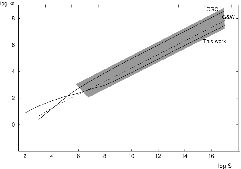
Figure 9.  : The $\Phi$ nondimensional convective flux as a function of $S$ for the present work, for the CGC model, for the mlt formula of Gough and Weiss (1976), and the observational limits deduced by Spruit (1974) (dashed area). The mlt fluxes were nondimensionalized assuming $l=H_{P}$.

In Figure 9 the $S$-dependence of the nondimensional convective flux

$$\Phi=\frac{2\pi}{S}\int_{0}^{\infty}dk\int_{0}^{\pi}n_{S}(\mbox{\bf k})\alpha(\mbox{\bf k})F(\mbox{\bf k})k^{2}\sin\theta\,d\theta$$ (49)

is shown. For comparison, the CGC result and some mixing-length theory (mlt) calibrations (with the choice $l=H_{P}=D$ as length scale) are also shown. It should be noted though that a direct comparison of the present Boussinesq model with mlt models of the strongly stratified solar convective zone is not necessarily sensible. The computed curve lies near the lower limit derived by Spruit (1974) and is by a factor of 7 lower (at large $S$ values) than the isotropic CGC curve. Similarly, the total specific kinetic energy

$$K=\pi\int_{0}^{k_{max}}dk\int_{0}^{\pi}F(\mbox{\bf k})k^{2}\sin\theta\,d\theta$$ (50)

(Figure 10) and the turbulent viscosity

$$\nu_{t}=2\pi\int_{0}^{k_{max}}dk\int_{0}^{\pi}\frac{F(\mbox{\bf k})k^{2}}{n_{c}(\mbox{\bf k})}\sin\theta\,d\theta$$ (51)

(Figure 11) are also considerably lower than the isotropic results. From these results the coefficient of the $K$–$\epsilon$ relation

$$\epsilon=\xi_{3}K^{2}/\nu_{t}$$ (52)

is found to be $\xi_{3}=0.184$, which is a factor of two higher than the experimental value. Similarly, for Smagorinsky’s constant we get $C\simeq 0.001$, to be compared with the latest experimental value of 0.003 (quoted by CGC). As in CGC, the agreement of the computed coefficients with the experimental ones to within a factor of 2 or 3 indicates that the qualitative behavior of $n_{S}(\mbox{\bf k})$ is typical for a general class of mechanisms generating turbulence.

Figure 10.  : The $K$ specific turbulent kinetic energy as a function of $S$.

Figure 11.  : The $\nu_{t}$ turbulent viscosity as a function of $S$.

Section 5 CONCLUSION

The application of the homogeneous anisotropic incompressible turbulence model desribed in Section 2 has shown that the anisotropy of turbulent thermal convection does not grow indefinitely with incresing $S$, but it rather saturates to a finite (and moderate) limiting value. This result is in agreement with numerical experiments but it is in contradiction with earlier theoretical expectations based on linear stability analysis. It remains to be seen how the inhomogeneity (nonlocality) of turbulence will influence these results, but it appears that the assumption of near isotropy is not the main factor limiting the validity of present-day convection theories.

The computations show that the resulting $\Phi$ convective flux is practically insensitive to the value of the $Q$ quenching parameter, unless $Q\ll 1$. The physical reason for this is that the flux is predominantly determined by the low wavenumber energy-containing eddies, so details of the quenching at higher wavenumbers do not have serious effects on it. The comparison with numerical experiments shows that $Q$ is indeed of order unity. The low sensitivity of $\Phi$ to $Q$ means that the $\Phi^{\prime}optoS^{1/2}$ scaling remains valid for any form of the (unknown) $Q(S)$ function. As the $Q$ parameter basically determines the efficiency of the coupling between different velocity components (the “toroidal” and “poloidal” components of Massaguer, 1991), it follows that the secondary instabilities generating toroidal motions do not significantly influence the energy transport.

The work reported here has been the first attempt to study anisotropic turbulent convection in a self-consistent (though approximate) way. It is needless to say that further, more sophisticated models are necessary to extend these studies, in particular to the inhomogeneous case.

Acknowledgement

I am grateful for Carole Jordan’s encouragement. This work was partly funded by a Soros/FCO grant and by the OTKA grant No. 2135.

References

- Batchelor, G. K., The Theory of Homogeneous Turbulence (Ch. 2.4), Cambridge University Press (1953).
- Brandenburg, A., Moss, D., Rieutord, M., Rüdiger, G. and Tuominen, I., “-dynamos”, in The Sun and Cool Stars: activity, magnetism, dynamos (Eds. I. Tuominen, D. Moss and G. Rüdiger), Springer, p. 147 (1991).
- Canuto, V. M., “AMLT: anisotropic mixing-length theory”, Astron. Astrophys. 217, 333 (1989).
- Canuto, V. M., “The mixing-length parameter ”, Astron. Astrophys. 227, 282 (1990).
- Canuto, V. M., Goldman, I. & Chasnov, J., “A model for fully developed turbulence”, Phys. Fluids 30, 3391 (1987). (CGC)
- Canuto, V. M., Hartke, G. J., Battaglia, A., Chasnov, J. & Albrecht, G. F., “Theoretical study of turbulent channel flow: bulk properties, pressure fluctuations, and propagation of electromagnetic waves”, J. Fluid Mech. 211, 1 (1990)
- Chan, K. L. and Serizawa, K., “On numerical studies of solar/stellar convection”, in The Sun and Cool Stars: activity, magnetism, dynamos (Eds. I. Tuominen, D. Moss and G. Rüdiger), Springer, p. 15 (1991).
- Chan, K. L. and Sofia S., “Turbulent compressible convection in a deep atmosphere IV: Results of three-dimensional computations”, Astrophys. J. 336, 1022 (1989).
- Gough, D. O. and Weiss, N. O., “The calibration of stellar convection theories”, Mon. Not. R. A. S. 176, 589 (1976).
- Leslie, D. C., Developments in the Theory of Turbulence (Ch. 15.3), Clarendon (1973)
- Massaguer, J. M., “Stellar convection as a low Prandtl number flow”, in The Sun and Cool Stars: activity, magnetism, dynamos (Eds. I. Tuominen, D. Moss and G. Rüdiger), Springer, p. 57 (1991).
- Narasimha, D. and Antia, H. M., “Consistency of the mixing-length theory”, Astrophys. J. 262, 358 (1982).
- Nordlund, Å. and Dravins, D., “Stellar granulation III: Hydrodynamic model atmospheres”, Astron. Astrophys. 228, 155 (1990).
- Petrovay, K., “Morphology of convection and mixing-length theory”, Astrophys. J. 362, 722 (1990).
- Petrovay, K., “Topological pumping in the lower overshoot layer”, in The Sun and Cool Stars: activity, magnetism, dynamos (Eds. I. Tuominen, D. Moss and G. Rüdiger), Springer, p. 65 (1991).
- Rüdiger, G., Differential Rotation and Stellar Convection, Gordon & Breach, New York (1989).
- Spruit, H. C., “A model of the solar convective zone”, Solar Phys. 34, 277 (1974).
- Stein, R. F. and Nordlund, Å., “Topology of convection beneath the solar surface”, Astrophys. J. Lett. 342, L95 (1989).
- Xiong, D.-R., “A statistical theory of non-local convection”, Chinese Astron. 4, 234 (1980).