Primordial nucleosynthesis with massive $\tau$ neutrinos

Abstract

A massive long-lived $\tau$ neutrino in the MeV regime modifies the primordial light-element abundances predicted by big-bang nucleosynthesis (BBN) calculations. This effect has been used to derive limits on $m_{\nu_{\tau}}$. Because recently the observational situation has become somewhat confusing and, in part, intrinsically inconsistent, we reconsider the BBN limits on $m_{\nu_{\tau}}$. To this end we use our newly developed BBN code to calculate the primordial abundances as a function of $m_{\nu_{\tau}}$ and of the cosmic baryon density $\eta$. We derive concordance regions in the $\eta$-$m_{{\nu}_{\tau}}$-plane for several sets of alleged primordial abundances. In some cases a concordance region exists only for a nonvanishing $m_{{\nu}_{\tau}}$. At the present time BBN does not provide clear evidence for or against a $\tau$ neutrino mass.

1 Introduction

The theory of big-bang nucleosynthesis (BBN) describes the creation of the light elements hydrogen, helium, lithium, and beryllium in the early universe. The standard version of this theory is based on three main assumptions. 1. The evolution of the universe is described by the homogeneous and isotropic Friedmann-Robertson-Walker model. 2. The standard model of particle physics is used. 3. The lepton asymmetry of the universe is of the same order as the baryon asymmetry so that the chemical potential of the neutrinos in the early universe is small relative to the temperature.

Figure 1: Predicted values for the primordial abundances of the light elements assuming 2 (dashed), 3 (solid), and 4 (dotted) light neutrino families. The boxes indicate observationally inferred limits (Sect. 2).

Because the nuclear reaction rates and the neutron half-life are well known, there remains only one free parameter, namely the present-day cosmic number density $\eta$ of baryons relative to photons. For a given $\eta$ it is then possible to solve numerically a nuclear network in the expanding universe which gives the primordial light element abundances. In Fig. 1 we show the results of such a calculation for $10^{-10}<\eta<10^{-9}$, based on our newly developed BBN-code which is documented in [Rehm (1996)]. The results agree very well with those of other groups (e.g. [Yang et al. (1984)]; [Smith et al. (1993)]).

Table 1: Observationally inferred primordial light-element abundances. “Measured” values and the errors are taken from the given papers in which references to the original observations can be found. The errors are systematic except for those with the superscript “stat” (for statistical). For ${\rm{{}^{7}Li}}$ two sets of systematic errors are given as explained in the text.

Abundance	Measurement	Adopted Range	Label	Reference
$Y_{\rm p}$	$0.234\pm 0.003^{\rm stat}\pm 0.005$	0.223–0.245	l${\rm{{}^{4}He}}$	[Olive & Scully (1996)]
	$0.243\pm 0.003^{\rm stat}$	0.237–0.249	h${\rm{{}^{4}He}}$	[Izotov et al. (1997)]
${\rm D/H}\times 10^{5}$	$1.6\pm 0.2$	1.8–4.4	ISM	[Linsky et al. (1993)], [Dearborn et al. (1996)]
	$19\pm 4$	15–23	hQAS	[Rugers & Hogan (1996)]
	$2.3\pm 0.3^{\rm stat}\pm 0.3$	1.4–3.2	lQAS	[Tytler et al. (1996)]
${\rm{{}^{7}Li}}/{\rm H}\times 10^{10}$	$1.6\pm 0.07^{{\rm stat\,}+0.4+1.6}_{{\phantom{\rm stat\,}}-0.3-0.3}$	0.9–3.7	${\rm{{}^{7}Li}}$	[Fields et al. (1996)]

In the past, BBN has become a cornerstone of the hot big bang scenario in that one could find a concordance interval for $\eta$ where all observed light-element abundances agreed with the calculated values. Further, BBN has been used to constrain new particle-physics models, notably the properties of neutrinos, and thus has become a powerful tool in the field of particle astrophysics (e.g. [Malaney & Mathews (1993)]). In particular, if $m_{\nu_{\tau}}$, the mass of the $\tau$ neutrino, is larger than a few $100\,\rm keV$ the cosmic expansion rate during the BBN epoch is modified enough to cause significant changes in the predicted light-element abundances. Therefore, one can derive constraints on a putative mass for the $\tau$ neutrino or other neutral leptons that might be present in the early universe ([Dicus et al. (1978), Miyama & Sato (1978), Kolb & Scherrer (1982), Dolgov & Kirilova (1988)]).

Since this earlier works, the $m_{\nu_{\tau}}$ question has been revisited by many groups of authors ([Kolb et al. (1991), Dolgov & Rothstein (1993), Kawasaki et al. (1994), Dolgov et al. (1996)], Hannestad & Madsen 1996a,b, [Fields et al. (1997)]). The measured width of the $Z^{0}$ boson shows that there are exactly three neutrinos which are lighter than half the $Z^{0}$ mass so that the post-1990 works indeed focus on the question of a $\tau$ neutrino mass rather than on the number of light neutrino flavors or the mass of some arbitrary new lepton. One motivation for the post-1990 works was to understand the impact of certain approximations for the kinetic treatment of massive neutrino freeze-out. Another motivation was to include the latest observationally inferred primordial light-element abundances in the derivation of the constraints. While the treatments by the various groups differ in detail, they all agree that $m_{\nu_{\tau}}$ above a few $100\,\rm keV$ is forbidden. A mass beyond a few $10\,\rm MeV$ would again be allowed by BBN, but is experimentally ruled out (ALEPH–collaboration [Buskulic et al. (1995), Passalacqua (1996)]).

Meanwhile, the observational situation has changed in that the first direct measurements of deuterium in quasar absorption systems have become available. Unfortunately, the results by different authors and from different systems do not agree with each other, and do not necessarily agree with the classic interstellar-medium determination of the primordial abundance. In addition, a new determination of the primordial ⁴He abundance yields a significantly higher value than the previous “standard” result. Therefore, at the present time it is not clear which set of observational data (if any of the currently available ones) should be used to compare with the BBN calculations. It is not even clear whether there indeed exists any concordance interval for $\eta$, and if so, where exactly it lies. This constitutes the current debate about a possible “BBN crisis” (see [Hata et al. (1995), Copi et al. (1995)]).

Therefore, while the most recent papers on the $m_{\nu_{\tau}}$ question have focused on various aspects of the kinetic treatment for these particles during and after freeze-out, the main current source of uncertainty for $m_{\nu_{\tau}}$ limits is actually the observational situation. The main purpose of the present note is to reconsider BBN limits on $m_{\nu_{\tau}}$ in the light of the current debate about the correct primordial light-element abundances. In this regard our study is motivated by a similar discussion of the allowed number of massless neutrino species ([Cardall & Fuller (1996)]).

These authors have calculated the primordial light-element abundances as a function of the cosmic baryon-to-photon ratio $\eta$, and of the equivalent number of massless neutrino species $N_{\rm eff}$ which characterizes the energy density and thus the expansion rate of the universe at the time of BBN. They have then derived detailed concordance regions in the $\eta$-$N_{\rm eff}$-plane where different sets of observational data agree with the calculated abundances. However, these results cannot be trivially translated into concordance regions in the $\eta$-$m_{\nu_{\tau}}$-plane because the contribution of a massive tau neutrino to the expansion rate cannot be expressed in terms of an equivalent $N_{\rm eff}$, as we will discuss below. Therefore, it is best to construct such concordance regions directly in the $\eta$-$m_{\nu_{\tau}}$-plane. Before the onset of the current observational debate this sort of analysis was performed by [Kawasaki et al. (1994)].

A rather complete numerical treatment of the $\nu_{\tau}$ kinetics was performed in the works of [Kawasaki et al. (1994)] and Hannestad & Madsen (1996a,b). Together with the recent studies by [Dolgov et al. (1996)] and [Fields et al. (1997)] they indicate that the final concordance regions in the $\eta$-$m_{\nu_{\tau}}$-plane are rather insensitive to fine points of the $\nu_{\tau}$ kinetics. Therefore, we limit ourselves to the simplest approximation in which kinetic equilibrium is assumed for $\nu_{\tau}$ throughout so that an analytically integrated Boltzmann collision equation can be used. With this approach we can reproduce previous results with sufficient accuracy.

Of course, on a timescale much longer than the BBN epoch (approximately 200 seconds), the $\tau$ neutrinos have to decay into relativistic particles to prevent the universe from becoming overdominated by $\tau$ neutrinos today (e.g. [Kolb & Turner (1990)]). We will not discuss the impact of neutrino decays on BBN. Extensive previous discussions include those by [Kawasaki et al. (1994)] and [Dodelson et al. (1994)].

We begin our study in Sect. 2 with a short review of the current status of the observations. In Sect. 3 we describe the influence of a massive $\tau$ neutrino on the cosmic expansion rate, which is calculated by solving a simplified Boltzmann equation. In Sect. 4 the influence of a massive $\tau$ neutrino on the primordial abundances is studied. We derive concordance regions in the $\eta$-$m_{\nu_{\tau}}$-plane for different sets of observational data. Finally, we discuss and summarize our results in Sect. 5. Some details about the neutrino reaction rates are given in Appendix A.

2 Observations

In order to derive concordance intervals for the cosmic baryon density, or in order to derive BBN limits on novel particle-physics models, one must compare the calculated light-element abundances with observations. For most elements the difficulty is to derive the primordial abundances from values which are measured today in our vicinity. Even for ${\rm{{}^{4}He}}$, where this appears to be relatively straightforward and model-independent, some controversy has emerged. Therefore, we begin with a discussion of the current observational situation.

Helium-4

A large number of measurements exist for the ${\rm{{}^{4}He}}$ as well as for the O and N abundances in low-metallicity HII regions. Using O or N as tracers, the ${\rm{{}^{4}He}}$ abundance is extrapolated to zero metallicity to obtain the primordial value. We quote the usual “standard” value (“low ${\rm{{}^{4}He}}$” labeled l${\rm{{}^{4}He}}$ in Table 1) according to [Olive & Scully (1996)]. Their results are very similar to those of [Olive & Steigman (1995)]; the values and errors differ at most by $2\times 10^{-3}$. In contrast, [Izotov et al. (1997)] have found a significantly higher value (h${\rm{{}^{4}He}}$ in Table 1) using a new set of emissivities and collisional enhancement factors for the analysis of the observed spectral lines and by using other selection criteria for the HII regions. Their method and interpretation of the differences, in turn, has been critiqued by [Olive et al. (1997)], who reconfirm the above “low” value.

We emphasize that we do not give more weight to any of the two values; we merely quote what is currently discussed in the literature. In view of the disagreement between the lower deuterium value inferred from quasar observations (see below) it has been proposed that the systematic uncertainties might be substantially larger than commonly assumed ([Sasselov & Goldwirth (1995)]). They argue that the primordial mass fraction of ⁴He might be as high as 0.26.

Deuterium

For deuterium, there is the canonical value from observations of deuterium in the solar system ([Geiss (1993)]) and the interstellar medium ([Linsky et al. (1993), Linsky & Wood (1996), Piskunov et al. (1997)]) which provide a lower limit on the primordial deuterium abundance. Based on the theory of galacto-chemical evolution for deuterium, an upper limit—usually about a factor of 2–3 higher (cf. [Edmunds (1994)])—can be inferred. The most recent analysis is that of [Dearborn et al. (1996)] which is labeled “ISM” in Table 1. In all canonical models of galacto-chemical evolution a strong overproduction of ³He with respect to observations in the solar system and the ISM is found. As long as this problem remains unsolved, limits based on an analysis of the sum of deuterium and ³He should not be used to constrain the primordial abundances. The value quoted here relies on deuterium depletion only. Non–canonical models for stellar evolution, including additional mixing on the Red Giant Branch avoid a net production of ³He in low mass stars and might provide a solution to this problem ([Charbonnel (1995), Weiss et al. (1996)]).

In addition, deuterium is the only case where one believes to observe a primordial abundance directly. Deuterium lines were found in extragalactic HII clouds which lie on the line of sight to high redshift quasars (Quasar Absorption Systems or QAS). Unfortunately, the values found in different systems by different authors do not agree. [Tytler et al. (1996)] argue that the correct value is one order of magnitude smaller (“low QAS value” labeled lQAS in Table 1) than the one originally found by [Songaila et al. (1994)] and [Carswell et al. (1994)]. Their high value (hQAS in Table 1) was recently confirmed in an analysis by [Rugers & Hogan (1996)]. The high QAS deuterium abundance would allow for an $\eta$ concordance interval at relatively low values when combined with the lower ${\rm{{}^{4}He}}$ abundance, but poses severe problems for the theory of galacto-chemical evolution of deuterium and ${\rm{{}^{3}He}}$ (e.g. [Steigman (1994), Galli et al. (1995)]). Even the non-canonical models of [Charbonnel (1995)] and [Weiss et al. (1996)] cannot make the high deuterium value consistent with the present–day ³He observations. It is argued by [Songaila et al. (1994)], [Carswell et al. (1994)], and [Tytler et al. (1996)] that the high QAS deuterium value is in fact not deuterium, but another hydrogen cloud at a different position which mimics the deuterium line, and that the systems used are not sensitive for abundances as low as $10^{-5}$. This interpretation is rejected by [Rugers & Hogan (1996)]. Clearly, more high redshift quasar spectra are needed to reveal the true primordial deuterium abundance.

Lithium-7

The chemical evolution of lithium in stars is not well understood and therefore the derivation of the primordial value is much more uncertain. We quote here a recent value from [Fields et al. (1996)], based on the observations by [Molaro et al. (1995)], for the so-called “Spite plateau”, which is the minimal ${\rm{{}^{7}Li}}$ abundance found in old Pop II halo stars of our galaxy. Since it is nearly constant in stars with a surface temperature of more than 5500 K and metallicities lower than about 5 % solar, it is usually argued that this is the primordial value. Because the abundance depends on the modeling of the stellar atmosphere, the error is dominated by systematic effects (first set of systematic errors in Table 1). Furthermore, it has been suggested that ${\rm{{}^{7}Li}}$ might have been depleted significantly ([Deliyannis et al. (1990), Pinsonneault et al. (1992)]), but the detection of the more fragile isotope ${\rm{{}^{6}Li}}$ in two of these stars may be taken as an indication against strong depletion ([Steigman et al. (1993)]). The possible depletion effect is represented by the second set of systematic errors in the ${\rm{{}^{7}Li}}$ abundance.

The current observational evidence is summarized in Table 1. For each observation we also give a range for the relevant abundance which we have adopted to compare with the calculations below. The adopted range has been derived by adding the stated systematic error linearly with the $2\,\sigma$ statistical one. For lithium, both systematic errors have been linearly added. These procedures are somewhat arbitrary, but represent the common practice in this field.

Figure 2: Evolution of the parameter $g_{*}(t)$ for a Majorana $\tau$ neutrino with $m_{\nu_{\tau}}=10$, 20, and $100\,\rm MeV$ (solid lines). For comparison, the evolution of $g_{\ast}$ for 2 and 3 massless neutrino families is also shown (dotted lines).

3 Massive long-lived $\tau$ neutrinos in the early universe

As a further ingredient for our study of possible BBN limits on $m_{\nu_{\tau}}$ we need to specify the contribution of a massive neutrino to the expansion rate of the early universe. In the radiation dominated phase the expansion rate is governed by the Friedmann equation without a curvature term

$$H^{2}=\frac{8\pi}{3}\,\frac{\varrho}{m_{\rm Pl}^{2}}.$$ (1)

Here, $H=\mathaccent 31071{R}/R$ is the expansion rate, $m_{\rm Pl}$ the Planck mass, and $\varrho$ the energy density in radiation. It is commonly expressed in the form

$$\varrho=\frac{\pi^{2}}{30}g_{*}T^{4}$$ (2)

where $T$ is the cosmic temperature and $g_{*}$ the effective number of thermally excited relativistic degrees of freedom. This parameter is a function of temperature and thus of cosmic time. Just before the BBN epoch one finds

$$g_{*}=g_{\gamma}+\textstyle{\frac{7}{8}}\left(g_{e}+2N_{\nu}\right)=10.75$$ (3)

with $g_{\gamma}=2$ for the photons, $g_{e}=4$ for the electrons and positrons, and $N_{\nu}=3$ for the number of neutrino families which are assumed to be massless.

A particle species no longer contributes when $T$ falls below its mass because then its number density is suppressed and therefore the contribution to the cosmic energy density in the early radiation dominated phase of the universe is negligible. The evolution of $g_{*}$ in the temperature range $10^{2}$ to $10^{-2}$ MeV is shown in Fig. 2 (dashed lines) for a scenario with 2 and 3 light neutrino families. At a temperature of about 1 MeV the electrons get nonrelativistic and annihilate to photons. Therefore they drop out of Eq. (3), $g_{*}$ decreases, and their entropy is transferred to the photons, which dominate the energy density from now on.

Massive neutrinos contribute differently to the cosmic energy density than massless ones. Therefore, the expansion rate as a function of temperature and thus the time-temperature relation is modified, leading to changed light-element abundances in a BBN calculation. We examine a scenario where the $\tau$ neutrino is massive whereas the other two neutrinos are taken to be massless. Thermodynamic equilibrium is maintained as long as reactions such as

$$\nu_{\tau}+\bar{\nu}_{\tau}\longleftrightarrow a+\bar{a}$$ (4)

are fast compared to the expansion of the universe. Here, $a$ stands for any fermion which is kinematically allowed. As the universe expands, this reaction slows down and eventually the number density of $\tau$ neutrinos freezes out and stays constant thereafter (Fig. 3).

Figure 3: Number density (upper panel) and energy density (lower panel) as a function of the cosmic temperature for a $10\,\rm MeV$ Majorana $\tau$ neutrino. The contribution of a massless neutrino is shown for comparison. The densities are relative to those of photons and normalized to 1 at high temperatures. At $e^{+}e^{-}$ annihilation the photon density increases and the relative neutrino densities take a downward step as indicated. The curves marked “Equilibrium” represent the $\nu_{\tau}$ densities if the $\bar{\nu}_{\tau}\nu_{\tau}$ annihilations would not freeze out.

The process of freeze-out is described by the Boltzmann collision equation. This integro-differential equation is very difficult to solve in general, but it can be simplified by making the following approximations: 1. The annihilation products are in thermodynamic equilibrium due to effective interactions with the cosmic plasma. 2. Classical instead of quantum statistics is used, i.e. a Maxwell-Boltzmann distribution instead of a Fermi-Dirac or a Bose-Einstein one. 3. Even after annihilations the $\tau$ neutrinos are kept in kinetic equilibrium by effective elastic scatterings with electrons and massless neutrinos which are far more abundant. Other authors have dropped some or all of these assumptions, but the results do not change drastically, as we will discuss in Sect. 4. Because of the assumed kinetic equilibrium, the distribution function of the massive $\tau$ neutrinos can be expressed in terms of the so-called pseudo chemical potential $z_{i}$,

$$f_{\nu_{\tau}}=\exp\left(z_{i}-\frac{E_{i}}{T}\right).$$ (5)

Furthermore, the Boltzmann equation is integrated over the phase space of one of the incoming $\tau$ neutrinos. Because we assumed classical statistics, this can be done in a closed form and one arrives at one single ordinary differential equation for the $\nu_{\tau}$ number density,

$$\frac{{\rm d}n_{\nu_{\tau}}}{{\rm d}t}+3Hn_{\nu_{\tau}}=\left\langle\sigma v\right\rangle\;\left[n_{\nu_{\tau}}(t)^{2}-n_{\nu_{\tau}}^{\rm eq}(t)^{2}\right].$$ (6)

Here, $H$ is the expansion rate, $n_{\nu_{\tau}}$ the actual and $n_{\nu_{\tau}}^{\rm eq}$ the equilibrium number density of $\tau$ neutrinos. The thermally averaged reaction rate $\langle\sigma v\rangle$ is given in Appendix A.

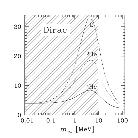
Figure 4: Number of effective light neutrino families $N_{\rm eff}$ equivalent to the contribution of a massive neutrino. The value of $N_{\rm eff}$ depends on the light element it is based upon. For Dirac neutrinos, our “helicity approximation” causes $N_{\rm eff}$ to be overestimated for $m_{\nu_{\tau}}\,\hbox{\raise 2.15277pt\hbox{$<$} \kern-10.00002pt\lower 2.58334pt\hbox{$\textstyle{\sim}$}}\,10\,\rm MeV$; this region has been hatched as a warning.

For a Dirac neutrino we are confronted with another difficulty because it has four degrees of freedom. In the massless case, only two of them interact with other particles, namely the helicity-minus neutrino and the helicity-plus antineutrino. The other two degrees of freedom are sterile and have no impact at all. If neutrinos have a mass, their helicity eigenstates are no longer eigenstates of chirality and thus are no longer completely sterile. The strength of the weak interaction for “wrong-helicity” neutrinos is suppressed by a factor of about $(m_{\nu_{\tau}}/2E_{\nu_{\tau}})^{2}$ relative to the usual rates, provided that $m_{\nu}\ll E_{\nu}$. In this case the quasi-sterile states remain essentially unexcited, leaving us with two degrees of freedom which are relevant for the cosmic expansion (for a recent discussion of cosmic abundances of right-handed neutrinos with masses up to 200 keV see [Enqvist et al. (1997)]). Conversely, for nonrelativistic neutrinos all four degrees of freedom interact with the full strength. Therefore, if the neutrino mass exceeds about $1\,\rm MeV$ so that they are nonrelativistic at the time of freeze-out, all four degrees of freedom would be fully excited and would thus contribute to the expansion rate of the universe

A correct treatment of the intermediate-mass regime requires a detailed kinetic treatment of neutrino helicities (e.g. [Fields et al. (1997)]). Because this is a very significant complication we have limited ourselves to an approximation where it is assumed that all available helicity states are always fully populated, an assumption that we shall refer to as the “helicity approximation”. It implies that the number and energy density of light ($m_{\nu}\hbox{\raise 2.15277pt\hbox{$<$} \kern-10.00002pt\lower 2.58334pt\hbox{$\textstyle{\sim}$}}1\,\rm MeV$) massive Dirac neutrinos is overestimated by a factor of 2. In the mass range from 1 – 10 MeV the number and energy density is still overestimated, but now by a factor less than 2; for $m_{\nu}\hbox{\raise 2.15277pt\hbox{$>$} \kern-10.00002pt\lower 2.58334pt\hbox{$\textstyle{\sim}$}}10\,\rm MeV$ our approximation yields the correct result.

Because we have assumed kinetic equilibrium, the energy density of the $\tau$ neutrinos can be calculated from their number density. As an example we show in Fig. 3 the evolution of the number and energy density, respectively, for a $10\,\rm MeV$ Majorana $\tau$ neutrino. Even though the neutrino mass causes the universe to become quickly matter dominated, we continue to parameterize the impact on the expansion rate by $g_{*}$ which thus no longer represents the effective number of relativistic degrees of freedom. It is merely a time-dependent proportionality factor between $T^{4}$ and the energy density according to the definition in Eq. (2).

4 BBN with massive $\tau$ neutrinos 

4.1 The number of effective light neutrino species

It is common practice in the literature to parameterize the influence on BBN of a new particle by the equivalent number $N_{\rm eff}$ of light neutrino species. This is a useful parameterization for a particle which is relativistic during the entire period of BBN, i.e. down to $T\,\approx\,40$ keV or until about 200 seconds after the big bang. Such a particle contributes a fixed amount to the parameter $g_{*}$ during the relevant epoch. On the other hand, a particle which is or becomes nonrelativistic during the BBN epoch contributes to the expansion rate in the way discussed in the previous section and displayed in Fig 2, i.e. its contribution to $g_{*}$ varies with time. Evidently, the effect of a massive $\tau$ neutrino cannot be mapped on a constant shift of $g_{*}$ or on a fixed modification of $N_{\rm eff}$.

One can still define a useful $N_{\rm eff}$ parameter indirectly by comparing the modification of the calculated abundance of a certain light element, for example ⁴He, caused by a massive neutrino with that caused by a fixed modification of $g_{*}$. The synthesis of the light elements peaks at different times for the different elements. Therefore, defining $N_{\rm eff}$ in this way depends on the chosen isotope. In Fig. 4 we show $N_{\rm eff}$ based on the equivalent impact on the abundances of deuterium and the two helium isotopes. (Note that in the Dirac case the low-mass range does not converge to the correct value of 3 light families, but to 4. This represents the abovementioned helicity approximation.)

In the previous literature $N_{\rm eff}$ has always been defined by the equivalent impact on ⁴He. However, if one wishes to perform a more direct comparison with different sets of observational data, there is no reason to introduce $N_{\rm eff}$. We will present all of our results directly as a function of $m_{\nu_{\tau}}$ in a form analogous to that used by [Kawasaki et al. (1994)].

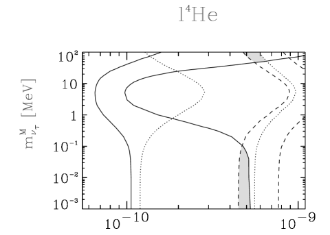
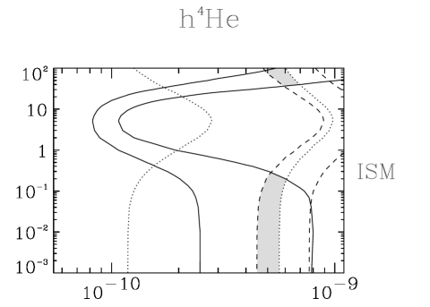
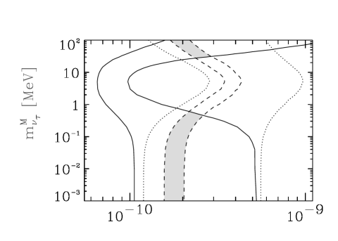
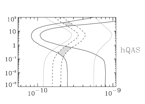
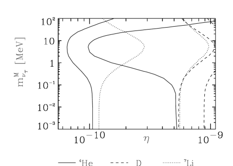
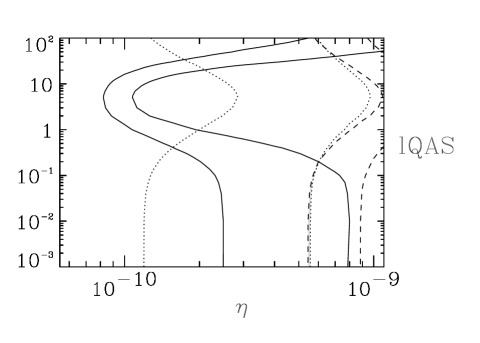
Figure 5: Isoabundance contours for the light elements if the neutrino mass is taken to be of Majorana type. In each panel, the contours have been drawn for a specific combination of observational data which are denoted according to the labels given in Table 1. (Left column: low ${\rm{{}^{4}He}}$. Right column: high ${\rm{{}^{4}He}}$. Top row: deuterium from ISM. Middle row: high deuterium from QAS. Bottom row: low deuterium from QAS.) The concordance regions for $\eta$ and $m_{\nu_{\tau}}$ are shaded.

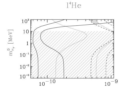
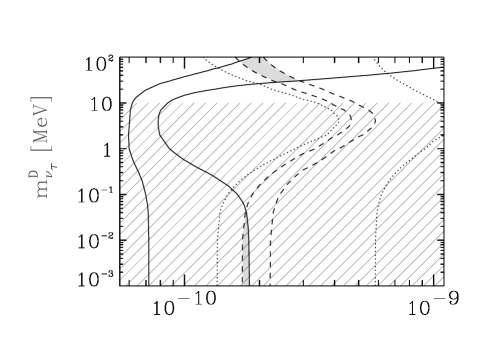
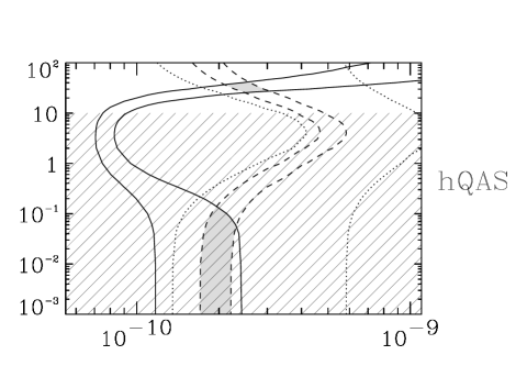
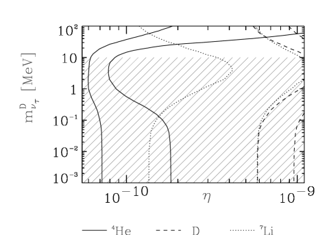
Figure 6: Isoabundance contours as in Fig. 5 if the neutrino mass is of Dirac nature. In the hatched area the results are not quantitatively correct because of our “helicity approximation”.

4.2 Validity of the approximated Boltzmann equation

The $N_{\rm eff}$ parameter remains very useful to compare our results with those of other authors who have dropped some or all of the simplifying assumptions made in Sect. 3 to calculate the neutrino freeze-out. [Fields et al. (1997)] used the integrated version of the Boltzmann equation, but with correct Fermi-Dirac statistics for the neutrinos. Furthermore, they did not assume thermodynamic equilibrium for the electron neutrinos, but solved the coupled Boltzmann equation for all three neutrino families and took into account the influence of the increased $\nu_{\rm e}$ number density on the weak reaction rates. This changes the maximum value of $N_{\rm eff}$ by about 0.5, but the limits on the allowed $\tau$ neutrino mass are hardly affected, because below $N_{\rm eff}=4$ the results practically coincide.

[Hannestad & Madsen (1996a)] (1996a,b) [Hannestad & Madsen (1996b)] solved the full Boltzmann equation for all neutrino species without any simplifying assumptions. In addition they calculated the influence of the deviation from equilibrium of the electron neutrino distribution function on the weak reaction rates. Their results deviate at most by 0.2 neutrino families compared to [Fields et al. (1997)].

[Dolgov et al. (1996)] solved the integrated Boltzmann equation with the method of the pseudo chemical potential only for the $\tau$ neutrinos, but calculated the deviation from equilibrium of the electron neutrino distribution function on the weak reaction rates. In this paper they do not present values for $N_{\rm eff}$, but only for $\Delta N_{\rm eff}$ relative to their earlier paper ([Dolgov & Rothstein (1993)]) for the results without $\nu_{\rm e}$-heating. There, very large values for $N_{\rm eff}$ were shown with $N_{\rm eff,max}^{\rm Dirac}\approx 11$ and $N_{\rm eff,max}^{\rm Majorana}\approx 8$. Their results for $\Delta N_{\rm eff}$ are opposite to those of the other groups. They argue that this is because [Fields et al. (1997)] did not take into account the deviation from equilibrium for the distribution function of the electron neutrinos, but [Kainulainen (1996)] showed in an update to [Fields et al. (1997)] that this would change their bounds by less than half a neutrino family.

In summary, the modifications of $N_{\rm eff}$ brought about by a more complete kinetic treatment of neutrino freeze-out and the weak interaction rates appear to be small enough to justify our simple treatment with the integrated Boltzmann equation.

In the study of [Kawasaki et al. (1994)] the $N_{\rm eff}$ parameter was not introduced, and they performed a rather complete numerical treatment of the $\nu_{\tau}$ kinetics. We have constructed a contour plot with the observational data used by [Kawasaki et al. (1994)] in order to be able to compare directly with their Figure 5(e) which refers to the stable Majorana neutrino case. Our contours agree with theirs better than we would have expected, corroborating that our simple approximation is entirely justified for the task at hand.

4.3 Concordance Regions

In Figs. 5 and 6 we present our results as isoabundance contours in the plane of baryon density vs. neutrino mass. In each panel, contours are drawn for ⁴He (solid), deuterium (dashed) and ⁷Li (dotted). The contour levels correspond to the adopted observational ranges listed in Table 1. Each panel corresponds to a specific combination of observational results as described in the figure. Concordance regions in the $\eta$-$m_{\nu_{\tau}}$-plane are shaded. In the Dirac case (Fig. 6) the area below about $10\,\rm MeV$ has been hatched because there our results are not quantitatively meaningful because of our helicity approximation. Qualitatively, the Dirac and Majorana cases, of course, yield rather similar results.

The Dirac $\tau$ neutrino results have to converge to the ones for the Majorana case in the small mass regime ($m_{\nu_{\tau}}\hbox{\raise 2.15277pt\hbox{$<$} \kern-10.00002pt\lower 2.58334pt\hbox{$\textstyle{\sim}$}}$ 1 MeV), since the “wrong-helicity” states are not populated there. In the intermediate mass range from 1 – 10 MeV our approximation still overestimates the contribution of the Dirac $\tau$ neutrino energy density to the cosmic expansion rate; the correct results for the light element abundances lie somewhere between the two cases .(For the ${\rm{{}^{4}He}}$ abundance in the presence of a massive Dirac $\tau$ neutrino with the correct treatment of the helicity states see [Fields et al. (1997)].) The correct treatment of both helicity states does not open up new concordance regions in this mass range.

The most recent experimental limit on the $\tau$ neutrino mass is $m_{\nu_{\tau}}<18$ MeV (ALEPH–collaboration, [Passalacqua (1996)]), somewhat lower than the previously published limit (ALEPH–collaboration, [Buskulic et al. (1995)]). Therefore, the concordance regions above this mass limit are already ruled out.

If the classic ISM determination of the primordial deuterium abundance were correct after all (top row in Figs. 5 and 6) we would be left with a concordance region in the low-mass regime; in fact the neutrino mass may well be zero in this case. Even though the concordance region does not show up in the Dirac case because of our helicity approximation, it would be there because for low-mass neutrinos the Dirac and Majorana cases are equivalent. The concordance region is almost independent of which ⁴He result is used because of the constraints provided by the deuterium and lithium contours. A mass range between a few hundred keV and few tens of MeV is excluded.

If the high QAS deuterium abundance is correct (middle row in Figs. 5 and 6), the result depends on the assumed ⁴He abundance. If the low value is right, the situation is similar to that discussed in the previous paragraph, except that the inferred cosmic baryon abundance is smaller by a factor of 3. If the high helium abundance is the true value, then in the Majorana case there remains a small concordance region which actually requires a neutrino mass somewhat below $1\,\rm MeV$. In the Dirac case, the situation is unclear because of our helicity approximation.

If the low QAS deuterium abundance is taken to be the primordial one (bottom row in Figs. 5 and 6), there is essentially no concordance region whatsoever, independently of the neutrino mass. This situation would constitute a true “crisis for BBN” as there would be no consistency between observations and calculations. Some other novel ingredient would be needed besides a massive neutrino.

5 Summary

We have studied the influence of a massive $\tau$ neutrino in the MeV range on the primordial abundances of the light elements. Several recent studies indicate that our simple approximate treatment of the Boltzmann collision equation for the neutrinos is quite adequate. We have focussed on a comparison between the calculated light-element abundances with current observational data by virtue of contour plots in the $\eta$-$m_{\nu_{\tau}}$-plane. This method avoids the use of an effective number of neutrino families $N_{\rm eff}$ which cannot be defined simultaneously for all light element abundances.

We find that the existence and location of concordance regions where all observations can be reproduced depends dramatically on the assumption which of the abundances currently offered as the “observed primordial” ones are actually correct. Depending on ones choice or judgment one may find that BBN is in crisis (no concordance region at all), that a nonvanishing neutrino mass is required, or that there are concordance regions even for a vanishing neutrino mass.

In each case one finds that a neutrino mass between the experimental limit of 18 MeV and about 1 MeV (and a bit below) is ruled out. In this regard our conclusions agree with those of previous authors. In spite of the great uncertainty of the observational situation, this conclusion is rather stable because of the opposite curvature of the deuterium and the helium contours which peak in opposite $\eta$-directions for neutrino masses of a few MeV.

Still, given the unclear observational situation one cannot be confident in the reliability of such limits. After all, if there were no concordance region whatsoever so that a new ingredient for BBN would be required, the possible impact of this new physics on the present results is entirely unknown. One clearly has to wait until the mutual inconsistencies of the observationally inferred abundances have been sorted out before one can arrive at far-reaching cosmological conclusions about the properties of elementary particles.

Appendix A Annihilation rates for massive $\tau$ neutrinos

The reaction rate for $\tau$ neutrinos annihilating to fermions is given by the thermal average over the cross section $\sigma$ times the relativistic invariant relative velocity $v$ ([Gondolo & Gelmini (1991)])

$$\left\langle\sigma v\right\rangle = \frac{1}{4m_{\nu_{\tau}}^{4}TK_{2}^{2}(m_{\nu_{\tau}}/T)}$$

$$\int_{4m^{2}_{\tau}}^{\infty}{\rm d}s\;\sigma vE_{\nu_{\tau}}E_{\bar{\nu}_{\tau}}\sqrt{s-4m_{\nu_{\tau}}^{2}}K_{1}(\sqrt{s}/T).$$

$K_{i}$ is the modified Bessel function of the second kind of order $i$ as defined in [Abramowitz & Stegun (1972)], $E_{i}$ are the particle energies, $s=(P_{\nu_{\tau}}+P_{\bar{\nu}_{\tau}})^{2}$ is the center of mass energy, and $P$ are the four momenta. We borrowed the expression $\sigma vE_{\nu_{\tau}}E_{\bar{\nu}_{\tau}}$ from [Dolgov & Rothstein (1993)]. The expressions given there are misprinted in several ways as confirmed by the authors (private communication). The correct expressions must read for Dirac neutrinos

(8)

$$= \displaystyle{\frac{1}{4}\frac{1}{g_{{\nu}_{\tau}}g_{\nu_{\tau}}}\sum_{a}\sum_{\rm Spins}\int|M_{\nu_{\tau}\bar{\nu}_{\tau}\leftrightarrow a\bar{a}}|_{\rm D}^{2}}$$

$$\displaystyle{(2\pi)^{4}\delta^{4}(P_{\nu_{\tau}}+P_{\bar{\nu_{\tau}}}-P_{a_{1}}-P_{a_{2}})\frac{{\rm d}^{3}{\bf p}_{a}}{2E_{a}(2\pi)^{3}}\frac{{\rm d}^{3}{\bf p}_{\bar{a}}}{2E_{\bar{a}}(2\pi)^{3}}}$$

$$= \displaystyle{\frac{G_{\rm F}^{2}w}{4\pi}\sum_{a}\left[\frac{1}{6}\left(C_{{\rm V},a}^{2}+C_{{\rm A},a}^{2}\right)\left(s-m_{a}^{2}-m_{\nu_{\tau}}^{2}\frac{w^{2}}{s^{2}}\right)\right.}$$

$$\displaystyle{\left.+\;\frac{m_{a}^{2}}{s}\left(C_{{\rm V},a}^{2}-C_{{\rm A},a}^{2}\right)\left(\frac{s}{2}-m^{2}_{\nu_{\tau}}\right)\right]},$$

and for Majorana neutrinos

(9)

$$= \displaystyle{\frac{1}{4}\frac{1}{{g_{{\nu}_{\tau}}g_{\nu_{\tau}}}}\sum_{a}\sum_{\rm Spins}\int\frac{1}{2}|M_{\nu_{\tau}{\nu}_{\tau}\leftrightarrow a\bar{a}}|_{\rm M}^{2}}$$

$$\times \displaystyle{(2\pi)^{4}\delta^{4}(P_{\nu_{\tau}}+P_{\bar{\nu_{\tau}}}-P_{a_{1}}-P_{a_{2}})\frac{{\rm d}^{3}{\bf p}_{a}}{2E_{a}(2\pi)^{3}}\frac{{\rm d}^{3}{\bf p}_{\bar{a}}}{2E_{\bar{a}}(2\pi)^{3}}}$$

$$= \displaystyle{\frac{G_{\rm F}^{2}w}{2\pi s}\sum_{a}\left\{\left(C_{{\rm V},a}^{2}+C_{{\rm A},a}^{2}\right)m_{\nu_{\tau}}^{2}\left(m_{a}^{2}-\frac{s}{2}\right)\right.}$$

$$+ \displaystyle{\left.\left(C_{{\rm A},a}^{2}-C_{{\rm V},a}^{2}\right)m_{a}^{2}\left(3m_{\nu_{\tau}}^{2}-\frac{s}{2}\right)\right.}$$

$$+ \displaystyle{\frac{1}{3s}\left(C_{{\rm V},a}^{2}+C_{{\rm A},a}^{2}\right)}\displaystyle{\left[\left.\frac{w^{2}}{2}\left(\frac{s}{2}-m_{\nu_{\tau}}^{2}\right)+\frac{s^{2}}{4}\left(s+2m_{a}^{2}\right)\right]\right\}}.$$

Here, p_i are the three momenta, $G_{\rm F}$ the Fermi-constant, $m_{a}$, $C_{{\rm V},a}$, and $C_{{\rm A},a}$ are the mass and the vector and axial couplings for the final state fermions. Further we have defined $w=(s^{2}-4sm_{a}^{2})^{1/2}$. The squared matrix element $|M_{\nu_{\tau}\bar{\nu}_{\tau}\leftrightarrow a\bar{a}}|^{2}$ is summed over the kinematically allowed reaction channels ($\nu_{\tau}\bar{\nu}_{\tau}\to e^{+}e^{-}$, $\nu_{e}\bar{\nu}_{e}$, $\nu_{\mu}\bar{\nu}_{\mu}$) and averaged over the spins.

References

- [Abramowitz & Stegun (1972)] Abramowitz M., Stegun I.S. (eds.), 1972, Handbook of mathematical functions, Dover Publications Inc., New York
- [Buskulic et al. (1995)] Buskulic D. et al., 1995, Phys. Lett. B 349, 585, (ALEPH Collaboration)
- [Cardall & Fuller (1996)] Cardall C., Fuller G.M., 1996, ApJ 472, 435
- [Carswell et al. (1994)] Carswell R.F., Weymann R.J., Cooke A.J., Webb K.J., 1994, Mon. Not. R. Astron. Soc. 268, L1
- [Charbonnel (1995)] Charbonnel C., 1995, ApJ 453, L51
- [Copi et al. (1995)] Copi C.J., Schramm D.N., Turner M.S., 1995, Phys. Rev. Lett. 75, 3981
- [Dearborn et al. (1996)] Dearborn D., Steigman G., Tosi M., 1996, ApJ 465, 887
- [Deliyannis et al. (1990)] Deliyannis C.P., Demarque P., Kawaler S.D., 1990, ApJ Suppl. Ser. 73, 21
- [Dicus et al. (1978)] Dicus D.A., Kolb E.W., Teplitz V.L., Wagoner R.V., 1978, Phys. Rev. D 17, 1529
- [Dodelson et al. (1994)] Dodelson S., Gyuk G., Turner M.S., 1994, Phys. Rev. D 49, 5068
- [Dolgov & Kirilova (1988)] Dolgov A.D., Kirilova D., 1988, Int. J. Mod. Phys. A 3, 267
- [Dolgov et al. (1996)] Dolgov A.D., Pastor S., Valle J., 1996, Phys. Lett. B 383, 193
- [Dolgov & Rothstein (1993)] Dolgov A.D., Rothstein I.Z., 1993, Phys. Rev. Lett. 71, 476
- [Edmunds (1994)] Edmunds M.G., 1994, Mon. Not. R. Astron. Soc. 270, L37
- [Enqvist et al. (1997)] Enqvist K., Keränen P., Maalampi J., Uibo H., 1997, Nucl.Phys.B 484, 403
- [Fields et al. (1997)] Fields B.D., Kainulainen K., Olive K.A., 1997, Astropart. Phys. 6, 169
- [Fields et al. (1996)] Fields B.D., Kainulainen K., Olive K.A., Thomas D., 1996, New Astronomy 1, 77
- [Galli et al. (1995)] Galli D., Palla F., Ferrini F., Penco U., 1995, ApJ 443, 536
- [Geiss (1993)] Geiss J., 1993, in: Origin and Evolution of the Elements (Edited by Prantzos N., Vagioni-Flam E., Cassé M.), p. 89, Cambridge, UK, Cambridge University Press
- [Gondolo & Gelmini (1991)] Gondolo P., Gelmini G., 1991, Nucl. Phys. B 360, 145