SPECTRAL ENERGY DISTRIBUTIONS OF GAMMA-RAY BLAZARS

Laura Maraschi

Osservatorio Astronomico di Brera, via Brera 28, 20121 Milano, Italy

Giovanni Fossati

Scuola Internazionale Superiore di Studi Avanzati, via Beirut 2–4, 34014 Trieste, Italy

ABSTRACT

Average Spectral Energy Distributions (SED) for different subgroups of blazars are derived from available homogeneous (but small) data sets, including the gamma–ray band. Comparing Flat Spectrum Radio Quasars (FSRQ) with BL Lacs extracted from radio (RBL) or X–ray surveys (XBL) remarkable differences and similarities are apparent: i) in all cases the overall SED from radio to gamma–rays shows two peaks; ii) the first and second peak fall in different frequency ranges for different objects, with a tendency for the most luminous objects to peak at lower frequencies; iii) the ratio between the two peak frequencies seems to be constant, while the luminosity ratio between the high and low frequency component increases from XBL to RBL and FSRQ. The variability properties, (amplitude and frequency dependence) are similar in different objects if referred to their respective peak frequencies. Finally, comparing spectral snapshots obtained at different epochs, the intensities of the two components at frequencies close and above their respective peaks seem to be correlated. The relevance of these properties for theoretical models is briefly discussed.

1. THE BLAZAR FAMILY

In 1978 Ed Spiegel proposed the name ”blazar” to designate a class of objects including BL Lacs as well as flat spectrum, radio loud quasars (Angel & Stockman, 1980). Although there are differences among members of the class, the underlying hypothesis was that at least the phenomena associated with the continuum derive from a common process, most likely a jet of relativistically moving plasma.

The opening of the high energy windows of X–ray and gamma–ray astronomy revealed further differences within the blazar family. X–ray astronomy led to the discovery of a new subclass, the so called X–ray selected BL Lacs, differing from the classical radio-selected BL Lacs in the relative strength of their X–ray and radio emissions and in a lesser degree of ”activity” in the radio to optical emission (e.g. Urry and Padovani, 1995).

More recently, the Compton Gamma Ray Observatory revealed that in many cases a substantial fraction and in some cases the bulk of the emitted power is released in this very high energy band. This fundamental discovery with far reaching theoretical implications extensively discussed at this meeting, poses the problem as to why some blazars are detected in gamma–rays and some are not, or in other words whether there are significant differences in the gamma–ray emission of different blazars.

In the following we will discuss the observed spectral energy distributions of blazars from radio to gamma–rays, and their variability, showing that there are clear systematic differences between the continua of different blazar subclasses. Nevertheless a unitary approach is still possible, maintaining a common process of energy release in a relativistic jet and relating the observed differences to different physical conditions in or around the jet.

2. SPECTRAL ENERGY DISTRIBUTIONS OF BLAZARS

Average spectral energy distributions of blazars have been constructed recently, taking advantage of the fact that the complete samples of the 1 Jy BL Lacs (RBLs), the EMSS BL Lacs (XBLs) and a small but complete sample of FSRQs (Brunner et al. 1994) have all been observed with the ROSAT PSPC allowing to derive ”uniformly” X–ray fluxes and in most cases spectral shapes in the 0.1 – 2 keV range (Sambruna et al. 1996a, and references therein). Average fluxes at radio, mm (230 GHz), IR and optical frequencies were taken from the literature.

The SEDs of each class, plotted in a $\nu F(\nu)$ vs. $\nu$ diagram, are smoothly convex up to the X–ray range and show a broad peak (Fig. 1). The peak frequency increases from FSRQs to RBLs and XBLs. The X–ray spectrum follows the general trend of continuous steepening only in the case of XBLs, while for RBLs and FSRQs the X–ray spectrum is flatter than the optical to X–ray extrapolation, suggesting a new spectral component. If RBLs are splitted into three subgroups according to the shape of their optical to X–ray continua (convex, straight or concave) the SEDs of the three subgroups at lower frequencies follow the same patterns as the three main groups, suggesting that we have to do with a continuous spectral sequence within the blazar family, rather than with separate spectral classes.

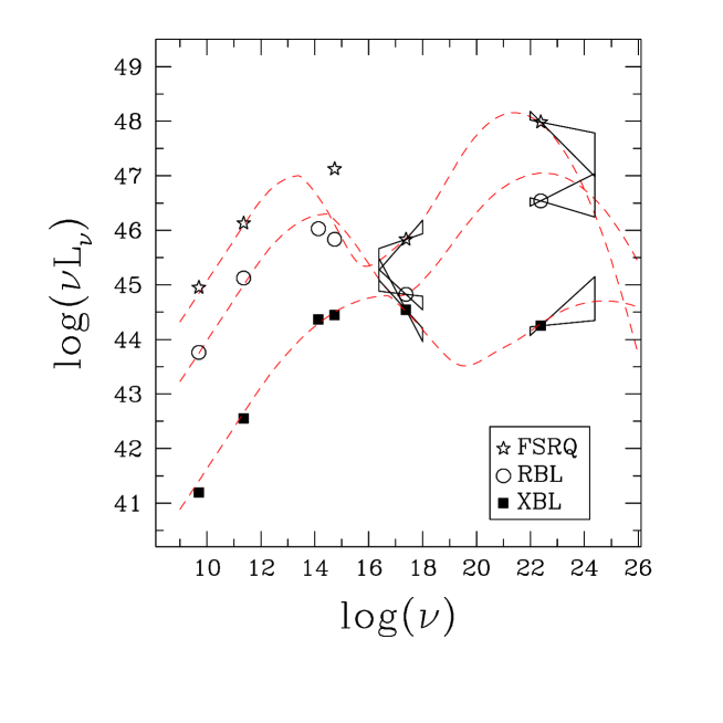
Figure 1: Spectral Energy Distributions of blazar subclasses. The points up to the X–ray range derive from average fluxes for complete samples of blazars (Sambruna et al. 1996a). The average slopes in the X–ray range are also shown. Average gamma–ray intensities and spectral shapes were obtained from results by Comastri et al. (1997) as explained in the text. The dashed lines are analytic approximations to the SEDs meant to merely ”describe” the observed trends.

Unfortunately the gamma–ray observations are at present less ”systematic”. In order to add average gamma–ray fluxes and spectral indices to the SEDs for XBLs, RBLs and FSRQs we will use the correlation between gamma–ray properties and X–ray properties found by Comastri et al. (1997) for 37 FSRQs, 11 RBLs and 5 XBLs with measured fluxes in both bands (see also Ghisellini this volume). For the joint sample, the gamma to X–ray flux ratio is strongly correlated with the radio to optical flux ratio, characterized by the two point spectral index $\alpha_{RO}$. Based on the above correlation we assign a gamma–ray flux to each subclass according to the average $\alpha_{RO}$ parameter of the class, the average X–ray flux for the class and the gamma to X–ray flux ratio defined by the correlation of Comastri et al. (1997). In addition we plot for each class the average spectral shape in the 0.1 – 5 GeV band measured by the EGRET experiment on board CGRO for the above objects.

The results are shown in Fig. 1, admittedly very preliminary, but highly suggestive. Clearly a second peak is present in the SED of each subgroup in a very broad gamma–ray range. The location of this second peak can be guessed from the shape of the gamma ray spectrum. Depending on whether the gamma–ray spectrum is steep , medium or flat ($\alpha_{\gamma}>1,\simeq 1,<1$), the peak must fall below within or above the EGRET range.

The dashed curves in Fig. 1 are drawn mainly to guide the eye. However we mention that the low frequency part is a parameterization discussed in Fossati et al. (1996) based on the hypothesis that the peak frequency of the first spectral component is inversely related to the luminosity in this component ($\nu_{peak}\propto L^{-1.5}$ in this case). The only point deviating strongly from the analytical description is the optical flux of FSRQ. While this discrepancy could be real, we note that for the 8 objects in the sample, the adopted magnitudes probably have large errors, since these objects were scarcely observed and the magnitudes used were mostly retrieved from the Véron-Cetty & Véron catalog (Véron-Cetty & Véron, 1993).

The lines describing the second spectral component, peaking at very high frequencies have been drawn assuming that the second peak frequency has a fixed ratio ($10^{8}$ to the first one and a height proportional to the average radio luminosity of each subclass. It is remarkable how well the average X–ray spectra fit into this very simple scheme.

Summarizing: the SEDs of blazars show two broad peaks. The first can fall between $10^{14}-10^{17}$ Hz, the second between $10^{22}-10^{25}$ Hz depending on the object. However for a given object the two peak frequencies are correlated, the present data being compatible with a constant ratio. The strength of the gamma–ray peak with respect to the lower frequency one increases with increasing $\alpha_{RO}$.

3. VARIABILITY AND SPECTRAL ENERGY DISTRIBUTIONS

The above properties can be verified in several, diverse, prototype objects for which also variability data have been obtained, namely 3C 279, a weak lined FSRQ (Maraschi et al. 1994), Mrk 421, a typical XBL (Macomb et al. 1995, 1996), and PKS 0528+134, a typical strong lined FSRQ (Sambruna et al. 1996b). We can summarize the comparison of broad band spectral snapshots obtained at different epochs for each object, stating that the variability is similar in all these objects, once the different peak frequencies of their spectral components are taken into account. More explicitly, in all cases the variations are larger and the spectra tend to be harder in higher intensity states at frequencies larger than the peak frequencies of the two spectral components. For instance a hardening is seen clearly in the IR to UV continuum of 3C 279 ($\nu_{peak,1}$ falls in the FIR) and in the X–ray spectrum of Mrk 421 ( $\nu_{peak,1}$ falls in the soft X–ray band). In Mrk 421 a hardening is observed also in the high energy spectrum, where the TeV emission varies more than the GeV emission ($\nu_{peak,2}\simeq 100$ GeV. In PKS 0528 +134, the gamma–ray slope measured by EGRET is $>1$ ($\nu_{peak,2}\simeq 100$ MeV) and flattens significantly at high intensity. It is remarkable that a shift by three decades to lower frequencies of the Mrk 421 data yields a very good match with the high and low gamma–ray spectra of PKS 0528+134.

Finally it is important to stress that as long as one considers the energy ranges above each peak (at $\nu_{peak,1}$ and $\nu_{peak,2}$), where the largest variability is observed, the intensities of the high and low energy branch in the same object vary in a correlated fashion. We are not aware of any counterexample to this behaviour.

4. GENERAL THEORETICAL CONSIDERATIONS

The above properties strongly support models involving synchrotron and Inverse Compton radiation in a relativistic jet to account for the two components in the SEDs. The arguments are i) that the spectral shapes of the two components are ”similar” as expected for synchrotron and IC radiation from the same relativistic electrons (except for effects of self–absorption); ii) the two components vary in a correlated fashion. On the other hand present observations are insufficient to decide whether the seed photons are the synchrotron photons themselves (SSC) or photons present outside the jet (External Compton, EC) (see for a review Sikora 1994, and refs. therein).

Comparative spectral fits with both models to the same data and a discussion of the expected correlations in the two cases can be found in Ghisellini et al. (1996) and Maraschi and Ghisellini (1996). Briefly, if the variations are due to changes in the relativistic electron spectrum, the SSC model or the “mirror model” of Ghisellini and Madau (1996) predict that the Compton branch varies more than the corresponding synchrotron branch, while in the EC model the variations should be proportionate. However if the bulk Lorentz factor of the emitting region changes, the EC model variability can mimic the SSC one, and intermediate cases are possible if other parameters vary as well.

Short time scale variability at different frequencies (i.e. multifrequency light curves as obtained thus far for the BL Lac object PKS 2155–304, observed simultaneously with ASCA, EUVE and IUE, Urry et al. 1996; and for Mrk 421 observed simultaneously by the Whipple observatory, ASCA, EUVE and from ground, Buckley et al. 1996) offers the best means to discriminate between models. However the problem is complicated in practice by the necessity of taking into account the ”structure” of the source, as indicated by the ”delays” observed in the above sources. This is a new territory which needs to be explored (see the papers by Mastichiadis and Ghisellini in this volume).

A final comment concerns the trends in the SEDs shown in Fig. 1. The astrophysical cause of this trend is presently unknown. Ideas under discussion involve self–limited acceleration in the presence of strong radiative losses (Fossati et al. 1996) or different external (or intrinsic) physical conditions for the jet development (Sambruna et al. 1996b).

It would be extremely important to determine the physical parameters of the emitting region. If the SSC model applies to the three subclasses, then the constant ratio between the two peak frequencies implies that the energy of the relativistic electrons radiating at the peak $(\gamma_{e})^{peak}$ is the same in all objects. Consequently the magnetic field should be lower in objects with higher luminosity, peaking at lower frequencies (i.e. FSRQ).

If the spectral sequence correponds to the increasing dominance of the external radiation field (with constant, typical, rest frame frequency $\simeq 10^{15}$ Hz), then, in order to maintain a constant ratio between the observed peak frequencies, $(\gamma_{e})^{peak}$ should be lower in FSRQs and the magnetic field should be constant for the three subclasses.

References

Angel, J.R.P., & Stockman, H.S. 1980, ARA&A, 18, 321

Buckley, J.H., et al. 1996, ApJ, in press

Brunner, H., Lamer, G., Worral, D.M., & Staubert, R., 1994, A&A, 287, 43

Comastri, A., Fossati, G., Ghisellini, G., & Molendi, S., 1997, ApJ, submitted

Fossati, G., Celotti, A., Ghisellini, G., & Maraschi L., 1996 M.N.R.A.S., submitted

Ghisellini, G., & Madau, P. 1996, M.N.R.A.S., 280, 67

Ghisellini, G., Maraschi, L., & Dondi, L., 1996, A&A in press.

Macomb, D.J., et al. 1995, ApJ, 449, L99

Macomb, D.J., et al. 1996, ApJ, 459, L111

Maraschi, L., et al. 1994, ApJ, 435, L91

Maraschi, L., & Ghisellini, G. 1996, Proc. of ”Variability of Blazars”, Miami Febr. 1996.

Sambruna, R.M., Maraschi, L., & Urry, C. M. 1996a, ApJ, 463, 444

Sambruna, R.M., et al. 1996b, ApJ, in press

Sikora, M. 1994, ApJS, 90, 923

Urry, C.M., & Padovani, P. 1995, PASP, 107, 803

Urry, C.M., et al. 1996, ApJ, submitted

Veron–Cetty, M.P. and Veron, P., 1993, ESO Scientific Report No. 13