X-ray properties of the distant cluster Cl0016+16

Abstract

We present X-ray data on the distant cluster Cl0016+16 (z=0.5545) from ROSAT PSPC and HRI observations and use them to study the physics of the intracluster medium (ICM) and the dynamical state of the cluster. The surface brightness distribution is not only described by a spherically symmetric model but also by a two-dimensional $\beta$-model fit. Subtracting an elliptical model cluster as defined by the best fit parameters of the two-dimensional model we find significant residuals, indicating an additional, extended X-ray source within the cluster. This source, likely to be a merging subcomponent of the cluster, coincides with a peak in the weak lensing mass map of Smail et. al. (1995). In the course of this analysis we present a new approach to quantify the significance of substructure in cluster X-ray images dominated by Poisson noise and smoothed with a Gauss filter.
We determine the radial mass profile integrated out to a radius of 3Mpc and find for the total mass of the cluster a value of $\sim 1.4-3.3\times 10^{15}$ M_⊙ and $\sim 4.5\times 10^{14}$ M_⊙ for the gas mass, yielding a gas–to–total mass ratio of 14 – 32%. There is no significant radial dependence of the gas–to–total mass ratio in the cluster.

1 Introduction

Cl0016+16 is with a redshift of z=0.5545 one of the best studied clusters of galaxies at higher redshifts. It has been target of observations in all wavelength. The cluster is very massive and, comparing it to nearby clusters, it certainly is most similar to the Coma cluster. It seems to be embedded in a large-scale-structure density enhancement at a redshift of approximately z=0.55 (Koo, 1981). This idea was recently strengthened by Hughes, Birkinshaw & Huchra (1995), who found a poor cluster in X-rays at a redshift of 0.5506 at about 8 arcmin distance from Cl0016+16.
It is an exceptional cluster, due to its high X-ray luminosity (L_x(2-10keV)=2.62$\times 10^{45}$erg/sec (Tsuru et al. 1996) at such a high redshift. Also the optical appearance of this cluster is different to other equally distant clusters. For a long time it was known to be a counter example for the Butcher-Oemler effect (Butcher& Oemler 1978) showing only a red, old population of galaxies.
Belloni& Röser (1996) (hereafter BR) recently found that the cluster has a high fraction of E+A galaxies, being responsible for the relatively high fraction of red light in the cluster’s galaxies. Wirth, Koo & Kron (1994) studied 24 cluster members with the HST, and found that the E+A galaxies seem to be more disklike than normal red galaxies.
Cl0016+16 is an ideal cluster for the observation of the Sunyaev-Zel’dovich effect, as it is very X-ray luminous and at a high redshift. The cluster was among the first three objects for which a detection of the effect has been claimed (Birkinshaw, Gull & Hardebeck 1984; Uson 1986; see also Rephaeli 1995).
In this paper we study the X-ray properties of Cl0016+16 using ROSAT/PSPC and HRI data. We give constraints on the radial total mass profile of the cluster and discuss its morphology and its dynamical state. Most probably Cl0016+16 is in the process of a merger. The smaller infalling component carries only a small fraction of the mass, and therefore the merger has probably a small effect on the overall dynamical equilibrium of the cluster.
Recently, a weak gravitational shear signal was detected in the cluster by Smail et al. (1995) (hereafter SEFE). They used this measurement to infer the gravitational mass of Cl0016+16. We compare our results on the cluster mass derived from the X-ray data with their weak gravitational lensing results.
Throughout the paper we use a Hubble constant of H₀=50km/sec/Mpc.

2 The observations

2.1 ROSAT HRI data

Cl0016+16 was observed by the ROSAT/HRI for 76593 sec (for a description of ROSAT see Trümper 1983, 1992). The observation was performed in two different periods, in January and June/July 1995 with exposure times of 5,917 sec and 70,676 sec, respectively. To correct for a possible offset between the two pointings, we use the QSO 0015+162 in the North of the cluster. We measure an offset of $6^{\prime\prime}$ in right ascention and $4^{\prime\prime}$ in declination between both positions of the QSO, and correct for it.
Fig.1. shows the HRI count rate image of Cl0016+16. The image covers the total energy range of the ROSAT telescope, 0.1-2.4keV.
The source in the North-East of the centre is not very significant, and does not have an optical counterpart (see also Fig.5.). The QSO 0015+162 lies outside of this plot but can be seen in Fig.1.

Figure 1: Contour Plot of the ROSAT HRI observation of Cl0016+16. The image is smoothed with a Gauss filter with a $\sigma$ of 6 arcsec. The lowest contour level is 1.3$\times 10^{-6}$cts/sec/arcsec². The spacing is linear with steps of 5.22$\times 10^{-7}$ cts/sec/arcsec².

2.2 The PSPC data

Cl0016+16 was observed for 43,157 sec with the ROSAT PSPC (for more detailed information see Hughes et al. (1995)). To obtain the best signal-to-noise-ratio for the detection of the cluster we select the photons in the 0.5 - 2 keV energy band (channels 52 to 201). The resulting count rate image for this energy range is shown in Fig.2. The image is vignetting corrected. The PSPC data show a much more regular appearance, partly coming from the larger point spread function (PSF) of the instrument in comparison with the HRI, and partly from the better statistics. The PSPC has a much lower background and a higher sensitivity (about a factor of three) compared to the HRI.
The most prominent point source in the image is QSO 0015+162, lying to the North of the cluster, approximately 3 arcmin from the centre. In the South, approximately 8 arcmin from the centre, one can see a clearly extended source which is another galaxy cluster at a redshift of z=0.5506 recently discovered by Hughes et al. (1995) in the same PSPC data.

Figure 2: Contour plot of the exposure corrected PSPC data of Cl0016+16. The image is smoothed with a variable Gauss filter. The largest $\sigma$ is 30 arcsec. The lowest contour line is $1\times 10^{-7}$cts/sec/arcsec² The spacing of the contour levels is 35% of the value of the lower one.

3 The spatial data analysis

3.1 The spherical symmetric fitting

For the data analysis we use EXSAS, the software system provided by MPE (Zimmermann et al. 1994). To study the global physical properties of the cluster we primarily use the PSPC data, because they trace the cluster X-ray emission to larger radii due to the higher signal to noise and better photon statistics. But we also present the results of analyzing the HRI data. With the PSPC data we have also checked for a possible hardness ratio variation of the X-ray emission across the PSPC cluster image and found no variation, implying that the soft energy band does not provide any particular extra information on the physical parameters of the cluster.
To obtain an approximate description of the X-ray surface brightness distribution, which allows to subsequently derive the main physical parameters of the cluster analytically, we use the so-called isothermal $\beta$-model (Cavaliere&Fusco-Femiano, 1976, 1981; Sarazin&Bahcall, 1977; Gorenstein et al., 1978; Jones&Forman, 1984), which describes the surface brightness $S(r)$ of a galaxy cluster assuming spherical symmetry

$$S(r)=S_{0}\left(1+\frac{r^{2}}{r_{c}^{2}}\right)^{-3\beta+1/2}+B$$ (1)

where $S_{0}$ is the central intensity, $r$ the radius, $r_{c}$ the core radius, $\beta$ a slope parameter of the radial surface brightness distribution, and $B$ the background surface brightness. The $\chi^{2}$-fitting results for the PSPC data are: $\beta=0.80^{+0.09}_{-0.07}$, $r_{c}=372^{+62}_{-52}$kpc$\equiv 50.5^{+8.4\prime\prime}_{-7.1}$ (for a summary see Tab.2). The surface brightness profile and the fit are shown in Fig3. The results for the HRI data are: $r_{c}=283_{-81}^{+140}$ kpc, $\beta=0.68^{+0.26}_{-0.1}$ (see also Tab.3). Serendipitous sources are extracted from the fitting. The best fit values of both data sets for the core radius and the $\beta$ are quite different, but the error bars have a large overlap (see Tab.2 and Tab.3). The discrepancy arises from the fact, that the HRI data do not trace the cluster out to such a large radius as the PSPC data, due to higher background and lower sensitivity.
Fitting this spherically symmetric profile to the image of Cl0016+16 has the disadvantage that it does not perfectly describe the slightly elliptical cluster. But it allows a simple analytic deprojection of the surface brightness profile of the cluster yielding the radial gas density profile. We will show later that the spherically symmetric approximation is a sufficiently good description for the determination of the gas mass and total mass profiles with errors that are smaller than relevant uncertainties like those of the temperature distribution of the intracluster medium (ICM). It can actually be seen also from the analysis of simulated clusters that a spherically symmetric $\beta$ model approximation generally leads to a good description of the shape of realistic clusters with errors of less than 20% (e.g. Schindler 1995; Evrard, Metzler & Navarro 1996). The analytic deprojection of the profile of equ. (1) leads to the density profile:

$$\rho(r)=\rho_{0}\left(1+\frac{r^{2}}{r_{c}^{2}}\right)^{-3\beta/2}~{}~{}.$$ (2)

For the central electron density we obtain 0.65$\times 10^{-2}$cm^-3 from the PSPC data, and 0.77$\times 10^{-2}$cm^-3 from the HRI data.
For the fitting we cut out regions of serendipitous sources, which clearly do not belong to the emission of the ICM itself.
The different fit parameters are correlated. For example the $\beta$ and the core radius are dependent on each other. But $\beta$ is also correlated to the background. A too low result in the background leads to a decrease of $\beta$, as the profile has to become shallower to overcome the difference of the wrong background result to the real one. Therefore we have carefully checked these sources of uncertainty and found in particular that our result for the background in the fit is in perfect agreement with the background determined independently in large regions outside the cluster with all detectable individual sources removed.

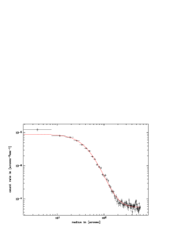
Figure 3: Surface brightness profile of Cl0016+16 from the PSPC data. The crosses mark the errors and the full line is the best fit with the parameters shown in Tab.2.

3.2 The two-dimensional fit

To account better for the slightly elliptical shape of the cluster we have also performed a two-dimensional fit to the cluster using a modified $\beta$ model that allows for two different core radii along the two principal axes of the cluster image ellipse. The surface brightness profile in this model is described by the equation:

$$S(r_{1},r_{2})=S_{0}\left(1+F_{1}+F_{2}\right)^{-3\beta+1/2}+B$$ (3)

with

$$F_{1}=\frac{(\mbox{cos}(\alpha)(r_{1}-x_{0})-\mbox{sin}(\alpha)(r_{2}-y_{0}))^{2}}{a_{1}^{2}}$$

$$F_{2}=\frac{(\mbox{sin}(\alpha)(r_{1}-x_{0})+\mbox{cos}(\alpha)(r_{2}-y_{0}))^{2}}{a_{2}^{2}}$$

The fit is applied to the two-dimensional pixel data of the image. The newly introduced parameters are defined in Tab.1.

Table 1: Description of the fit parameters of the two-dimensional case. Not mentioned parameters have the same definition as in the 1d fit.

parameter	definition
$x_{0}$	central position in x direction
$y_{0}$	central position in y direction
$r_{1}$	coordinate in x direction
$r_{2}$	coordinate in y direction
$\alpha$	position angle
$a_{1}$	major axis of core radius
$a_{2}$	minor axis of core radius

The results are shown in Tab.2 and Tab.3. This fit has the advantage of taking into account, that a relaxed cluster does not necessarily need to be completely spherical symmetric, but can show ellipticity. A further advantage is that the centre position of the cluster is derived in the fitting procedure itself and does not have to be predetermined like it is necessary in the one-dimensional analysis. There the centre position is usually determined from the maximum in the surface brightness profile (with some dependence on the smoothing used before determining the centre).
The application of such a two-dimensional fit can also be found in Bardelli et al. (1996) in which they apply this model to Abell 3558 the central cluster of the Shapley concentration.
However, the two-dimensional fit exhibits more problems than the one-dimensional one, firstly because of poorer statistics in each bin, as one has to use pixels instead of concentric rings. This is particularly severe at larger radii because the surface brightness is falling off steeply, which is partly compensated by the increasing surface of the rings in the one-dimensional analysis but not in the two-dimensional case. This is very crucial in the regions outside the cluster emission, where the only observed emission comes from the background. Secondly, the number of fit parameters increases from four to eight fit parameters.
For our two-dimensional fit we use the PSPC data with a binsize of $5^{\prime\prime}\times 5^{\prime\prime}$. We again cut out serendipitous sources in the field of view. Since the number of photons per pixel in the background area is too small to apply Gaussian statistics, which is assumed by $\chi^{2}$-fitting, we apply a small Gauss-filter to the image. The $\sigma$ of the Gauss-filter is $5^{\prime\prime}$, and therefore much smaller than the FWHM of the PSF ($\sim 30^{\prime\prime}$) of this data set, so that we do not risk to loose any information.
If we do not apply a Gauss-filter, we underestimate the background. This is due to the fact that for the low photon statistics in the background pixels the mean of the Poissonian distribution is larger than the most abundant value and the mean adopted by assuming a Gaussian distribution. This adopted Gaussian distribution is used with $\chi^{2}$-fitting. Because of the above mentioned correlation effect an underestimation of the background leads than to a decrease in the fitted slope parameter $\beta$. The application of a small Gauss filter improves the photons statistics and removes this problem. Of course, the errors obtained for the fitting parameters in this procedure are no longer precisely defined. However, it is a very good approach to get the best fit value. We test this with images on model clusters, on which we added Poisson noise. These model clusters have about the same parameters as Cl0016+16. We apply a Gauss-filter, of the same size as for the real cluster image, and run the fitting routine on them. The parameters obtained from the fitting are in very good agreement with the intrinsic model parameters, so that we can be sure, that the Gauss-filter does not obscure our fitting result.
The one-dimensional fit-parameters are in very good agreement with the two-dimensional fit-values (see Tab.2 and Fig.6), so that this can also be used as a proof for reliability of the Gauss filtering. The best fit value for the core radius in the one-dimensional fit is 372 kpc, lying almost exactly on the geometrical mean value of the 2d fit. Also the $\beta$ of the two fits agree very well, with 0.80 best fit value for the 1d fit, and the 2d fit being at 0.81.
Trying to overcome the Gauss filter with a larger binsize of the image is not feasible, due to the low background. The bins would be too large. The best fit value for from the two-dimensional fit are slightly depending on the binning. However, applying different binning and different Gauss filters (not too large of course) yields values which are all in excellent agreement with the 1d fit and its errors.
Another approach, using a maximum likelihood analysis, as for example applied by Birkinshaw, Hughes & Arnaud (1991), has the disadvantage of predefining the fit parameters. The parameters are not fitted, but only tested.
To check the existence of substructure, in addition to the overall ellipticity of the cluster, we produce a synthetic cluster image from the fit parameters of the two-dimensional model and subtract it from the real image. There is significant structure in the residual image that can indicate either point sources in the field or subcomponents of the cluster itself. The residual images are shown in Fig.4 for the PSPC data and in Fig.5 for the HRI data. To obtain Fig.5 the HRI image was treated in the same way as the PSPC image with a two-dimensional fitting approach. The used parameters are shown in Tab.3. Here the pixel size is $4^{\prime\prime}\times 4^{\prime\prime}$ and also $\sigma=4^{\prime\prime}$ for the Gauss filter. The residual images shown in these figures are displayed in the form of a significance plot. How the significance of the pixels of the residual images are calculated is explained in more detail in the appendix. Briefly the initial problem is how to calculate the significance of a source after having applied a Gauss filter. We solve this problem by using error propagation and Poisson noise. Basically two different Gauss filtered images are divided by each other. The one being the “error image”, is not only Gauss filtered, but also the square root of each pixel has to be calculated together with a general normalization. The “source image” can be calculated in two ways. In the first case one subtracts a background model. Then the routine gives $\sigma$ above background. The other possibility is to subtract a model cluster, and to calculate the significance ($\sigma$) of these residuals. A more general approach for the testing of significances with filter techniques (not only Gauss filters) is described by Rosati (1995).

4 The spectral analysis

Due to the spectral resolution of the PSPC it is possible to determine the temperature of the ICM. However, as this cluster has a very high redshift and only a relatively small number of source photons were detected, the spectral resolution is of course limited.
We determine the temperature in different radii around the centre of Cl0016+16 with different backgrounds and different energy bands with different values for metallicity. The results show a large scatter, which is due to the relatively low photon statistics. For example in a radius of 4 arcmin around the centre, the total sum of photons is about 6,000.
Nevertheless, the results which are in the range 6 to 10 keV are in quite good agreement with the ASCA data of Tsuru et al. (1996) who obtained a global temperature of $8.22^{+1.83}_{-1.47}$ keV. Only the results for the hydrogen column density are different. We obtain results of $4-6\times 10^{20}$cm^-2, which are in good agreement with the measurements of the 21cm line of $4\times 10^{20}$cm^-2(Dickey & Lockman 1990), while Tsuru et al. find $12.9\times 10^{20}$cm^-2. This difference might be explained by the fact, that ASCA does not provide a very good spectral sensitivity below 0.5keV, which is the energy range relevant for the determination of this degree of absorption.
In different rings (which are partly overlapping) we do not detect any significant temperature gradient, which leads us to the assumption that the cluster is probably more or less isothermal within the given the large error bars. This is in very good agreement with the ASCA data. Only in the very centre we see a drop of the lower boundary of the temperature (in a radius of 1 arcmin) to 4 keV together with an increase of the hydrogen column density. This decrease is, however, not significant and most likely an artifact of the temperature fitting, as the cluster has not yet developed a Cooling Flow (see also 5.2) for which such a temperature decrease would be expected. Therefore we neglect this lower boundary in the centre for the mass determination. Including it does not change the overall mass result significantly (the mean result changes by less than 5%).
In general it is interesting, that the temperatures determined from the PSPC data are only very weakly depending on the assumed values for the metallicity.

5 The Morphology of Cl0016+16

5.1 The X-ray data

Cl0016+16 shows a position angle of about 50^∘ (measured from North to East) and an eccentricity of about 0.18. There are clearly additional sources superposed on the elliptical cluster, both in the HRI and the PSPC observation.

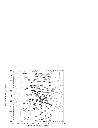
Figure 4: Significance of the residuals after subtracting the elliptical isothermal $\beta$-model from the original hard PSPC image. The parameters for the subtracted model is described in Tab.2. The stepsize of the contours is 1 $\sigma$. The dashed line is the 0 level, the full lines are positive the positive $\sigma$’s, the dotted ones are the negative ones. The numbers are the objects of the optical identification list of BR. The Gauss filter has a $\sigma$ of 25 arcsec.

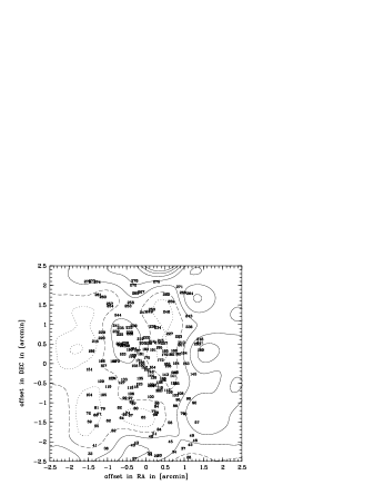
Figure 5: Significance of the residuals after subtracting the elliptical isothermal $\beta$-model from the original HRI image. The parameters are presented in Tab.3. The stepsize is 1 $\sigma$. The dashed line is the 0 level, the full lines are positive the positive $\sigma$’s, the dotted ones are the negative ones. The numbers are the objects of the optical identification list of BR. The Gauss filter has a $\sigma$ of 20 arcsec.

In the West of the cluster, about 2 arcmin from the centre (Fig.4), we find a surface brightness excess with 4 $\sigma$ significance in the PSPC image. This source at a position of RA=00H18M27S DEC=16D25M55S (J2000) is most likely extended, as explained in the discussion.
The residual image of the HRI observation also shows a surface brightness excess to the West of the centre. At the exact location of the PSPC maximum of Fig.4 we find, however a gap in the HRI surface brightness excess (Fig.5). There are several effects that can produce such a result. First of all, the HRI data have a lower photon statistics than the PSPC data as explained above and thus the gap may be produced by a larger statistical fluctuation (the surface brightness excess is just produced by 55 photons). The second point is, that only the hard band photons were used for the analysis of the PSPC data. We cannot apply the same selection to the HRI, as this instrument does not provide any energy discrimination. But as we found no significant feature in a hardness ratio map produced from the PSPC data we believe that the difference in the shape of the western emission excess is due to photon statistical effects.
Therefore we conclude, that there is an extended source in the West in the line-of-sight of Cl0016+16. This extended source might be a subgroup falling into this cluster. However, this subgroup, if existing is very small compared to the total cluster Cl0016+16.
Another source visible in the significance plot of the PSPC image, but only having a 2$\sigma$ significance, is the source in the South. This source structure is most likely to be extended too. Galaxy number 43, defined by BR, having a redshift of z=0.38, indicated in the figure, coincides with the maximum of this source, so that it might be, that there is emission from a small foreground group, as already suggested by Ellis et al. (1985). However, optical source number 36 also in this enhancement is a star and might contribute partly to the emission.

5.2 Cooling time

The central cooling time, calculated for a gas temperature of 8.4keV (Tsuru et al, 1996; Yamashita, 1995) and for the density profile obtained from the isothermal $\beta$ model fit is larger than 10¹⁰years from both the PSPC and the HRI data. Therefore the cluster cannot have yet formed a steady cooling flow (Fabian, Nulsen & Canizares 1984).

5.3 Comparison with optical data

Cl0016+16 is a well observed cluster in the optical. There has been an extensive survey by Dressler & Gunn (1992) (hereafter DG) and BR. Fig.4 and Fig.5 show the overlays of the optical data of the sample of BR.
We did not apply a bore-side correction in the PSPC image, but found an inaccuracy of the data of 2 to 5 arcsec for the pointing position.
The most striking feature is, that the alignment of the central galaxies is coinciding with the PA we determined from X-rays (as already mentioned by SEFE). However, for the 4 $\sigma$ excess emission in the West of the centre, which is probably a substructure feature of the cluster, there is not enough overlap with the data of BR to search for a possible galaxy density enhancement which could be related to the surface brightness excess. DG detected objects in that region, but they did not obtain redshifts for them. The objects seem to be extended, so that it is likely that they are galaxies.

6 Mass analysis

6.1 The one-dimensional approach

X-ray observations of the ICM in clusters of galaxies can be used for the determination of the total and gas mass. The formula for the cluster mass profile obtained from combining the isothermal $\beta$ formalism (1d) equ(2) and the hydrostatic equation is:

$$M(<r)=\frac{kr^{2}}{G\mu m}\left(\frac{dT}{dr}-\frac{3\beta rT}{r^{2}+r_{c}^{2}}\right)$$ (4)

The results are shown in Fig.6. For the mass determination we use the PSPC data because of the better statistics, even though the spatial resolution is a factor about 7 worse in comparison to the HRI data. Our total mass estimate for Cl0016+16 at a radius of 3Mpc is about 2.3$\times 10^{15}$ M_⊙ . This is a typical result for a rich cluster, like for example the Coma cluster of galaxies (Briel, Henry & Böhringer 1992).
For the mass determination we use the method by Neumann & Böhringer (1995). This method uses a Monte-Carlo approach for determining the cluster’s radial mass profile. The stepwidth for the Monte-Carlo method is 300kpc with a maximal change of the temperature of 1 keV per step. For the temperature range we take 6 to 10 keV (rounded errors of Tsuru et al. 1996 and our results from the PSPC data fitting). We assume that the cluster gas is not necessarily isothermal, but only that the gas temperature lies in the given temperature range. This assumption is justified since we find no significant temperature variations in different concentric rings. The gas mass of the cluster integrated out to a radius of 3 Mpc is roughly 4.5$\times 10^{14}$ M_⊙ . Thus we obtain a gas to total mass ratio of about 20%. This is in the typical range of other clusters.

6.2 The two-dimensional approach

With our results for the two-dimensional fit, it is also possible to determine the influence of ellipticity on the results for the cluster mass. For comparison we determine the masses with the major and minor-axis results for the core radius of the two-dimensional fit. We again use the Monte-Carlo approach with the same conditions as the one-dimensional analysis. As one can see, the difference between both results becomes less with increasing radius. This result is natural, as only the coreradius is different, which influences the mass result mostly near the centre.

6.3 Comparison of the different mass estimates

Comparing the different results for the total mass of the 1d approach with the 2d approach leads to similar results, as can be seen in Fig.6. This also implies that it is a good approach even to take only a sector out of a certain cluster surface brightness distribution when the cluster is elliptical. This approach has been normally undertaken, if clusters show clear substructure, to exclude those regions. Only within the innermost 1 Mpc there is some divergence of the mass depending on the core radius. However averaging the 2d distribution to a modified 1d distribution leads to a core radius (by taking the geometrical mean of the major and minor axis) of less than 1% difference to the coreradius originally derived by the 1d fit. This is a proof, that the 1d fit averages correctly over the eccentricity of a cluster. Also the similarity of the $\beta$’s of both approaches supports this.
A comparison of the results for the gas mass shows that this case is slightly more critical. Because of the dependence of the central density on $\beta$ and the coreradius, one yields different results for the approach with the values for the major and minor axis. Therefore an analysis, that takes into account only sectors of the X-ray distribution must be undertaken cautiously, not to overestimate or underestimate the mean coreradius. Taking the extreme values for the major and minor axis, we get a difference to the averaged value almost up to 20%.
However, averaging over the entire cluster with a 1d fit is a good approach as the averaged 2d central electron density is of the order of 1% different to the one from the original 1d approach. Therefore the differences of the averaged 1d approach to the original 1d fit are in the order of less than 1%, and only diverge to less than 1.5% at a radius larger than 2.5 Mpc.

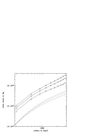
Figure 6: Integrated mass profile of CL0016+16. The full lines indicate the mass profile from the 1d fit. It shows the mean value and the upper and lower lines are the mean $\pm 2\sigma$. The small dots are the results for the 2d fit with the minor axis as core radius. The circles are the same for the major axis as core radius. Again middle values are the mean, the others $\pm 2\sigma$. The lower dotted line is the gas mass profile from the 1d fit, the dashed line is the gas mass from the 2d fit, using the major axis value as core radius, the dotted dashed line respectively for the minor axis result used as core radius.

Table 2: Obtained parameters for Cl0016+16 using the PSPC data. The physical values are all calculated with $H_{0}$ = 50 km/sec/Mpc. The errors for $r_{c}$ and $\beta$ from the 1d fit are 3$\sigma$ errors.

parameter	value
$\beta$ 1d fit	$0.80^{+0.09}_{-0.07}$
$r_{c}$ 1d fit	372${}_{-52}^{+62}$ kpc $\equiv 50.5_{-7.1}^{+8.4\prime\prime}$
$n_{e0}$ 1d fit	0.65 $\times 10^{-2}$cm-3
$M_{tot}<$ 3 Mpc	$2.32^{+0.94}_{-0.94}\times 10^{15}$ M⊙
$M_{gas}<$ 3 Mpc	$4.5\times 10^{14}$ M⊙
$\beta$ 2d fit	0.81
$r_{c}$ for major axis	410 kpc $\equiv 56^{\prime\prime}$
$r_{c}$ for minor axis	337 kpc $\equiv 46^{\prime\prime}$
PA (North over East)	50∘
$\epsilon$ (eccentricity)	0.18

Table 3: Obtained parameters for Cl0016+16 using the HRI data. The errors for $r_{c}$ and $\beta$ from the 1d fit are 3$\sigma$ errors.

parameter	value
$\beta$ 1d fit	$0.68^{+0.26}_{-0.1}$
$r_{c}$ 1d fit	283${}_{-81}^{+140}$ kpc $\equiv 38.5_{-11}^{+19\prime\prime}$
$n_{e0}$ 1d fit	0.76 $\times 10^{-2}$cm-3
$\beta$ 2d fit	0.69
$r_{c}$ for major axis	318 kpc $\equiv 43^{\prime\prime}$
$r_{c}$ for minor axis	261 kpc $\equiv 35^{\prime\prime}$
PA (North over East)	50∘
$\epsilon$ (eccentricity)	0.18

7 Discussion

7.1 Possible influence of the QSO on the X-ray temperature

Tsuru et al. (1996) found with ASCA a temperature of about 8.22keV and a very low metallicity, m$<$0.167 for the ICM. However, these values can in principal be obscured as there is another X-ray emitting source, QSO 0015+162 in the vicinity of the cluster (see also Fig.2). The distance to the cluster centre of 3 arcmin. This is in the order of the half power diameter of the point spread function of the ASCA plus GIS combination of 3.2 arcmin (Ikebe, 1996). Tsuru et al. 1996 used the GIS data. It is very likely, that this QSO, which has a redshift of z=0.553, close to the cluster’s redshift, influences the spectrum and therefore the spectroscopic estimates might be wrong. A rough estimate of the influence can be made by comparing the countrate of the QSO with the countrate of the cluster itself measured by ROSAT. For the PSPC we get a countrate of about 10% for the QSO in comparison to the cluster. Fitting a power law to the QSO spectrum of the PSPC yields a power law index in the range of -3 to -2.3. Fitting a power law to the cluster itself yields a power law index of -1.6 to -1.5, both times fixing the hydrogen column density to 5$\times 10^{20}$cm^-2. Thus the spectrum of the QSO is steeper implying that it has less influence in the higher energy band of ASCA. For the temperature measurement, the QSO would, if it influences the cluster spectrum, lower the fitted temperature, as fitting a Raymond-Smith spectrum to the QSO data yields a best fit parameter of about 2 keV.
Another possibility in principle is to measure the influence of the QSO to the cluster spectrum by comparing luminosities measured with ASCA and the PSPC. Tsuru et al. (1996) obtain a value for $L_{x}(2-10$keV$)=2.62\times 10^{45}$erg/sec. With the PSPC we get $L_{x}(2-10$keV$)=2.3-4.4\times 10^{45}$erg/sec. This shows that the errors are too large to give a definite result on the influence of the QSO. For the luminosity determination we took into account variations of the hydrogen column density, the metallicity and the temperature (6–10keV).
Taking this all together, it is not likely, that the QSO contributes sufficiently to the spectrum of the cluster, to explain the very low result for the metallicity. A 10% contribution to the continuum of the ICM spectrum probably does not lower the metallicity by a factor of two to three, which would be necessary, to make Cl0016+16 a ‘normal’ distant cluster, with a metallicity of about m=0.3.
The low value for the metallicity is rather surprising, as Cl0016+16 is the only cluster showing such a result. This does not fit in the normal scenario of metal enrichment, especially as the cluster exhibits many E+A galaxies (BR), which have already burned all O and B stars. These stars would have been in principle able to enrich the ICM by their supernovae. However, this does not seem to be the case.

7.2 The dynamical state of Cl0016+16

The X-ray image provides strong evidence for the existence of substructure in the cluster which is possible due to the merging of a galaxy group with the main cluster.
In this case, there are basically two possibilities to explain the observation, as suggested by simulations (Schindler & Müller 1993). The first one is, that the subgroup is on its first infall to the cluster, the second one is, that the subgroup already penetrated the cluster centre once.
The second scenario leads to a much stronger distorted appearance of the subgroup than the first one. As the subgroup can be seen as a more or less compact feature, the first case seems to be far more likely. Another very interesting feature is the chain of galaxies, which coincides very well with the PA of the gas. It is not clear whether this chain comes from a recent merger, and if, whether the measured substructure in the West has something to do with it. The merger direction of the substructure roughly agrees with the PA of the gas. This is a common feature for mergers as predicted by simulations (Van Haarlem & Van de Weygaert, 1993). However, it might also be, that the chain of galaxies are only the remnants of a former merger, proving that the cluster formed out of filaments.

7.2.1 Mass estimate of the possible subgroup

The subgroup in the West shows up with about 55 photons in the hard ROSAT/PSPC band of 0.52–2.01 keV.
Due to the limited number of photons, it is very difficult to give estimates on the physical quantities of this source. However, assuming this source is at the cluster’s redshift, and on its first infall to the cluster, so that it still contains most of its own X-ray emitting ICM, we obtain a X-ray luminosity of about $L_{x}\sim 10^{43}$erg/sec. Comparing this luminosity to groups of galaxies, we find, that this value is on the upper limit for Hickson groups (Ponman et al. 1996). Poor clusters of galaxies, having more galaxies than Hickson groups are lying in the regime of about 10⁴⁴erg/sec, depending if they are hosts for Cooling Flows or not. Therefore we can classify our source as a group of galaxies in the range between Hickson groups and poor clusters of galaxies. The mass range, which one observes for these objects lies in the order of 10¹³ M_⊙ to 10¹⁴ M_⊙ (Ponman et al. 1996; Mulchaey et al. 1996). This is the most likely mass range for the subgroup. Comparing this result with the total cluster mass of about 2$\times 10^{15}$ M_⊙ , we find a contribution of the subgroup to the total mass of about 1% to 20%.

7.2.2 Contamination by stars

It must be noted, however, that this additional source does not need to be a cluster group at the same redshift as Cl0016+16. It might be a chance alignment of two point sources, or it might be a group of galaxies at another redshift. A single point-source is pretty unlikely to be the case, as we can reject a point-like shape with a confidence limit of 99%. This confidence limit is determined by comparing the surface brightness distribution of the source with the surface brightness distribution of an artificial point-source having 55 photons (see also Fig.7). The surface brightness distribution is marginally affected by the (subtracted) model parameters and the pixel size of the image.
To exclude the possibility of an artifact produced by the satellite observatory (e.g. wobbling), we compare the quasar in the North of the cluster with a point source, again using the surface brightness distribution. We obtain very good agreement of the quasar with a point-source, again the artificial point source having the same number of photons than the quasar itself, after subtracting the cluster emission (note: the Poisson errors are calculated for the total number of photons per bin, not only for the residual photons). Inspecting the optical image we find at a distance of about half an arcmin a red star. This star is by far the brightest optical source in this region. It is a M4V dwarf (BR). We can calculate an upper limit for the X-ray luminosity of the star, using the magnitude of the luminosity in the red band of m_r=16.84, and m_v=18.5 in the visible (from the Cosmos data base). The saturation limit for M dwarfs is found to have a value of 10^-3 (Fleming et al. 1993). This value defines the upper limit of the energy radiated in X-rays versus the energy emitted in the optical for M dwarfs. The 55 excess photons found in the hard ROSAT band exceed this limit by a factor of 8, excluding this star as the source of the X-ray emission.
However, we cannot exclude Quasars or AGN’s to be the source, probably, if the case, in a chance alignment.
A strong indication for the existence of a group of galaxies in the West of the centre of the cluster can be found by comparison with the dark matter map obtained by SEFE using the weak lensing approach by Kaiser & Squires (1993).

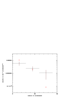
Figure 7: The surface brightness profile of the additional source in the West of the centre of Cl0016+16. The crosses mark the data, inclusive errors, the dots show the distribution of a point source having the same number of photons as the original residual source.

7.3 Comparison with weak lensing

Recently SEFE presented a map of the dark matter distribution measured by weak lensing. They also made a rough estimation of the mass inferred by X-rays, also using the ROSAT/PSPC data.
First of all, as SEFE already discussed, the PA of the mass distribution the light and the X-ray emission agrees well. Comparing our mass results with the SEFE mass estimates, however, yields a discrepancy. Our result of the projected mass is 4–7$\times 10^{14}$M_⊙ integrating out to a projected radius of 600 kpc, whereas SEFE derive a projected mass of 7.3$\times 10^{14}$M_⊙ using X-rays and a result for the weak lensing mass of 8.5$\times 10^{14}$ M_⊙ (depending on the mean redshift of the lensed background galaxies) out to the same distance. This discrepancy can be explained by using a different projection model for the X-ray surface brightness, which is more peaked in the centre than observed with the limited resolution of the PSPC data. Also shifting the lensed background galaxies to redshifts at 1$<$z$<$1.4 can in principle resolve the discrepancies. The fact that the background galaxies might be at a higher redshift than 1 is also supported by an observation of Luppino & Kaiser (1996). They measured the weak shear around MS1054-03, a rich and very X-ray luminous cluster at z=0.83 (Luppino & Gioia 1995), and found a mass-to-light ratio in agreement with more nearby clusters, when the lensed background galaxies lie at a redshift of about 1.5.
Comparing the morphology of the weak lensing mass map with our residual images yields very good overall similarities. The bimodality which can be seen in the weak lensing maps exhibits similarities as seen in Fig.4, and also less striking in Fig.5. The structure in the West found in the PSPC data coincides well with the western extension in the map of SEFE.

7.4 The gas to total mass ratio in Cl0016+16

Integrating over the entire cluster (outer boundary 3Mpc), the gas to total mass ratio of the cluster is 14–32%. This is calculated for the 1d fit. We did not take any uncertainties concerning the hydrogen column density into account. For the overall temperature we took 8.4 keV. These results are typical for clusters and undeline the effect of the Baryonic Catastrophe (Briel et al. 1992; White et al. 1993). The ratio does not vary very much with radius, it stays constant within the error bars.

7.5 The Eccentricity of Cl0016+16 and its consequences

In X-rays (ROSAT/PSPC and HRI data) Cl0016+16 shows an eccentricity of $\epsilon$ = 0.18. As HRI and PSPC show the same eccentricity, the larger PSF of the PSPC does not seem to affect this value. It is in good agreement with the optical distribution of the galaxies of $\epsilon_{gal}=0.21\pm 0.02$ derived by SEFE. The eccentricity is also comparable with results for other clusters like A2199 (Gerbal et al. 1992) and the sample of Buote & Canizares (1992) (hereafter BC). BC’s results on $\epsilon$ are generally smaller than the value for Cl0016+16, but this might be caused by the limited area they took into account for the determination (in all cases $<$ 1Mpc).
As we proof, the ellipticity of Cl0016+16 hardly affects the total mass profile of the cluster. The fact that the galaxy distribution and the X-ray surface brightness lead to similar eccentricities is a strong argument that we do not underestimate the eccentricity of the dark matter, despite the fact that SEFE obtain a result for the eccentricity of the dark matter of $\epsilon_{wl}=0.61\pm 0.06$ ($r<<r_{c}$) via the weak lensing approach of Kaiser & Squires (1993). This discrepancy might be caused by the limited area of the CCD’s for the lensing approach. Therefore it might be, that SEFE only measure the eccentricity in the centre, which is likely to be higher than the rest of the cluster, due to the chain of galaxies, and the results of BC, who found that clusters in X-rays tend to show a rounder appearance with increasing radius. It is also possible, that the eccentricity measured by SEFE is partly overestimated due to the clear bimodal shape of the dark mass map. Generally BC found out that X-rays are a good tracer for the shape of the dark matter, better than for example the galaxy distribution. However, the influences on the gas mass profile are relatively high (deviations of up to 20%). Thus taking for the gas mass estimate only sectors of the whole cluster can bias the results. This is an approach X-ray astronomers sometimes undertake, to eliminate regions which are strongly affected by substructure. However the differences are not drastic enough to change the gas-to-total-mass of the clusters dramatically.

8 Summary

In this paper we present X-ray properties on Cl0016+16, a distant cluster of galaxies with a high X-ray luminosity of L_X(2–10keV)=2.3–4.4$\times 10^{45}$erg/sec. The cluster has a temperature between 6-10keV. ASCA and ROSAT temperature results being well consistent. We present the total mass profile of the cluster based on X-ray measurements on ASCA and ROSAT, using a Monte-Carlo technique. The mass lies between 1.4–3.3 $\times 10^{15}$ M_⊙ integrated out to a radius of 3Mpc. The gas-to-total-mass ratio lies between 14-32%, making this cluster another example for the so-called Baryonic Catastrophe (Briel et al. 1992; White et al. 1993).
Applying a substructure analysis, we find indications for a not very massive group of galaxies falling into the centre of the cluster. This analysis is based on subtracting an elliptical model cluster following the isothermal $\beta$-model from the cluster X-ray image, with subsequent testing of the residuals. This indicates, that Cl0016+16 is not very disturbed. The PA’s of the distribution of the E and E+A galaxies, the weak lensing mass distribution, and the X-rays are coinciding very well with about 50^∘.

Appendix A The significance of sources with a Gauss filter

In this appendix we describe how we determine the significance of substructural features in a Gauss filtered image. The process of Gauss filtering can be described mathematically by:

$$G(x,y)=\left(\frac{1}{\sqrt{2\pi}\sigma}\right)^{2}$$ (5)

$$\int_{x}\int_{y}e^{-(x-x^{\prime})^{2}/2\sigma^{2}}e^{-(y-y^{\prime})^{2}/2\sigma^{2}}f(x^{\prime},y^{\prime})\mbox{d}x^{\prime}\mbox{d}y^{\prime}$$

$x$ and $y$ are the coordinates of the filtered and $x^{\prime}$ and $y^{\prime}$ the coordinates of the original image. The value of each pixel is described by $f(x^{\prime},y^{\prime})$. Applying the error propagation formalism to this function, assuming Poisson noise (i.e. $\Delta f(x,y)=\sqrt{f(x,y)}$), we obtain:

$$\Delta G(x,y)=\left(\frac{1}{\sqrt{2\pi}\sigma}\right)^{2}$$ (6)

$$\left(\!\int_{x}\!\!\int_{y}\!\!\left(\!e^{-(\!x\!-x^{\prime}\!)^{2}\!/\!2\!\sigma^{2}}\!\!e^{-(\!y\!-y^{\prime}\!)^{2}\!/\!2\!\sigma^{2}}\!\!f^{1\!/\!2}(\!x^{\prime}\!,\!y^{\prime}\!)\!\right)\!^{2}\mbox{d}x^{\prime}\!\mbox{d}y^{\prime}\right)\!\!^{1/2}$$

To realize this function one can apply a modified Gauss filter on the original image with a filter size of

$$\sigma^{\prime}=\frac{\sigma}{\sqrt{2}}~{}~{}.$$

and calculating the square root of this modified Gauss filtered image for each pixel and multiplying it with a factor of $\frac{1}{2\sqrt{\pi}\sigma}$. This gives $\Delta G(x,y)$. For the residual image the error $\Delta G(x,y)$ is the same as for the original smoothed image. Therefore to get the significance of the residuals one first calculates the subtracted count rate image by $G(x,y)-$Modell$(x,y)$ and calculates the statistical error of the residuals which is $\Delta G(x,y)$. The significance image is then

$$S(x,y)=\frac{G(x,y)-\mbox{Modell}(x,y)}{\ (x,y)}~{}~{}.$$ (7)

References

- [] Bardelli S., Zucca E., Malizia A., Zamorani G., Scaramella R., Vettolani, G., 1996, A&A, 305, 435
- [] Belloni P.,Röser H.-P., A&AS, in press
- [] Birkinshaw M., Gull S.F., Hardebeck H.E., 1984, Nature, 309, 34
- [] Birkinshaw M., Hughes J.P., Arnaud K.A., 1991, ApJ, 379, 466
- [] Briel U., Henry J.P., Böhringer H., 1992, A&A, 259, L31
- [] Buote D.A., Canizares C.R., 1992, ApJ, 400, 385
- [] Butcher H., Oemler A., 1978, ApJ, 219, 18
- [] Cavaliere A., Fusco-Femiano R., 1976, A&A, 49, 137
- [] Cavaliere A., Fusco-Femiano R., 1981, A&A, 100, 194
- [] Dickey J.M., Lockman F.J., 1990, ARA&A, 219, 18
- [] Dressler A., Gunn J.E. 1992, ApJS, 78, 1
- [] Elbaz D., Arnaud M., Böhringer H., 1995, A&A, 293, 337
- [] Ellis R.S., Couch W.J., MacLaren I., Koo D.C., 1985, MNRAS, 217, 239
- [] Evrard A.E., Metzler C.A., Navarro J.N., 1995, ApJ, submitted
- [] Fabian A.C., Nulsen P.E.J., Canizares C.R., 1984 Nat, 310, 733
- [] Fleming T.A., Giampapa M.S., Schmitt J.H.M.M., Bookbinder J.A., 1993, ApJ, 410, 387
- [] Gerbal D., Durret F., Lima-Neto G., Lachiéze-Rey, 1992, A&A, 253, 77
- [] Gorenstein P.D., Fabricant D., Topka K., Harnden F.R., Tucker W.H., 1978, ApJ, 224, 7188
- [] Hughes J.P., Birkinshaw M., Huchra J.P., 1995, ApJ, 448, L93
- [] Ikebe Y., 1995, Ph.D. Thesis, University of Tokyo
- [] Jones C., Forman W., 1984, ApJ, 276, 38
- [] Kaiser N., Squires G., 1993, ApJ, 404, 441
- [] Koo D.C., 1981, ApJ, 251, 75
- [] Luppino G.A., Kaiser N., 1996, ApJ, in press
- [] Luppino G.A., Gioia I., 1995, ApJL, 445, L77
- [] Mulchaey J.S., Davis D.S., Mushotzky R.F., Burstein D., 1996, ApJ, 456, 80
- [] Neumann D.M., Böhringer H., 1995, A&A, 301, 865
- [] Ponman T.J., Bourner P.D.J., Ebeling H., Böhringer H., 1996, in: X-Ray Imaging and Spectroscopy of Cosmic Hot Plasmas, F. Makino (ed.) in press
- [] Rephaeli Y., 1995, Ann. Rev. Astron. Astrophys., 33, 541
- [] Rosati P., 1995, Ph.D. thesis, University of Rome
- [] Sarazin C.L., Bahcall J.N., 1977, ApJS 34, 451
- [] Schindler S., Müller E., 1993, A&A, 272, 137
- [] Schindler S., 1995, A&A, 305, 756
- [] Smail I., Ellis R.S., Fitchett M.J. Edge A.C., 1995, MNRAS, 273, 277
- [] Squires G., Neumann D. M., Kaiser N., Arnaud M., Babul A., Böhringer H., Fahlman G., Woods D., 1996 submitted
- [] Trümper J., 1984, Adv. Space Res., 2, 241
- [] Trümper J., 1992, QJRAS, 33, 165
- [] Tsuru T., Koyama K., Hughes J.P., Arimoto N., Kii T., Hattori M., 1996, in: UV and X-ray Spectroscopy of Astrophysical and Labatory Plasmas, Yamashita K., Watanabe T. (eds.), Universal Academic Press, Tokyo, p.375
- [] Uson, J.M., 1986, Proc. of the conference on Radio Continuum Processes in Clusters of Galaxies, Green Bank, NRAO, p. 255
- [] Van Haarlem M., Van de Weygaert R., 1993, ApJ, 418, 544
- [] Wirth G.D., Koo D.C., Kron R.G., 1994, ApJ, 435, L105
- [] White S.D.M., Navarro J.F., Evrard A.E., Frenk C.S., 1993, Nat, 366, 429
- [] Yamashita K., 1994, in CLUSTERS OF GALAXIES eds. Durret, F., Mazure, A., Trân Than Vân, J., EDITIONS FRONTIERES, Gif-sur-Yvette, p.153
- [] Zimmermann H.U., Becker W., Belloni T., Döbereiner S., Izzo C., Kahabka P., Schwendtker O., 1994, EXSAS User’s Guide, MPE Report 257