Accretion of Cold and Hot Dark Matter onto Cosmic String Filaments

Abstract

The Zeldovich approximation is applied to study the accretion of hot and cold dark matter onto moving long strings. It is assumed that such defects carry a substantial amount of small-scale structure, thereby acting gravitationally as a Newtonian line source whose effects dominate the velocity perturbations. Analytical expressions for the turn-around surfaces are derived and the mass inside of these surfaces is calculated. Estimates are given for the redshift dependence of $\Omega_{nl}$, the fraction of mass in nonlinear objects. Depending on parameters, it is possible to obtain $\Omega_{nl}=1$ at the present time. Even with hot dark matter, the first nonlinear filamentary structures form at a redshift close to 100, and there is sufficient nonlinear mass to explain the observed abundance of high redshift quasars and damped Lyman alpha systems. These results imply that moving strings with small-scale structure are the most efficient seeds to produce massive nonlinear objects in the cosmic string model.

BROWN-HET-1049 June 1996.

hep-ph/yymmdd Typeset in REVTeX

I Introduction

The cosmic string model may be the most promising alternative to inflation-inspired theories of structure formation (see Ref. [1] for recent reviews). Many predictions of the model, for example a scale-invariant primordial spectrum of density perturbations[2] and the amplitude of cosmic microwave background (CMB) anisotropies on large angular scales[3], are at least qualitatively in agreement with observations.

The main problem facing the cosmic string model is the computational difficulty in analyzing its predictions. Cosmic strings will form during a phase transition in the very early Universe provided that certain well known topological criteria[4] are satisfied by the matter theory. It is also well established that the network of strings, once formed, will approach a “scaling” solution[5], i.e. the distribution of strings will become independent of time if all lengths are scaled to the Hubble radius.

However, the exact form of the scaling solution is not known. At any time $t$, there are two components to the string network: loops with radius $R\ll t$, and “long” string segments with curvature radius $R_{c}\sim t$. The best available numerical simulations [6] indicate that more mass is in the long strings than in loops. A further uncertainty pertains to the amount of small-scale structure which builds up on the long string segments as a consequence of the involved dynamics of the string network. Long straight strings with no small-scale structure carry no local gravitational potential. Their only effect is to lead to a conical structure of space perpendicular to the string[7]. Their transverse velocities will typically be close to the speed of light since the underlying dynamics is governed by the relativistic wave equation. Strings carrying small-scale structure, on the other hand, generate a local Newtonian potential[8] in addition to the conical distortion of space.

Given the lack of knowledge about the details of the initial string distribution, it is important to study all mechanisms by which strings can give rise to structures. Loops will produce roughly spherical objects by gravitational accretion[2], long strings without small-scale structure generate planar overdensities[9, 10], while long strings with small-scale structure induce - since they act as Newtonian gravitational line sources - filamentary objects[11, 12, 13].

In this paper we will study filament formation, i.e. the accretion of both cold dark matter (CDM) and hot dark matter (HDM) onto a moving Newtonian line source, by means of the Zeldovich approximation[14] and its suitable adaptation to HDM[15]. The Zeldovich approximation is a Lagrangian perturbation technique which is an improvement over standard linear perturbation theory and is widely applied in cosmology.

The accretion of CDM onto static string loops was analyzed a long time ago[16]. Subsequently, it was realized[17, 18] that - in contrast to theories based on adiabatic perturbations - the cosmic string model also appears viable if the dark matter is hot. The effects of string loops on HDM were then analyzed carefully[17, 19] by solving the collisionless Boltzmann equation, i.e. keeping track of the entire phase space distribution of the dark matter particles. Studies of nonlinear clustering about static string loops were also performed[20] by means of N-body simulations. At the time when string loops are produced, they typically have relativistic velocities. Hence, it is important to study the accretion of dark matter by moving seeds. Bertschinger[21] applied the Zeldovich approximation to study the case of CDM. He found that the total nonlinear mass is to a first approximation independent of the velocity $u_{i}$ of the loop. The decrease in the width of the nonlinear region is almost exactly compensated by the increase in the length of the structure. The study of clustering onto moving string loops was recently[22] generalized to HDM. In this case, the total nonlinear mass was shown to decrease with increasing $u_{i}$. Nevertheless, it was demonstrated that sufficient accretion to form nonlinear objects by a redshift of $z=4$ takes place.

Since the string network simulations indicate that long string would be more important for structure formation than loops, attention turned to the formation of string wakes. The accretion of CDM was analyzed in detail by means of the Zeldovich approximation in Ref. [23]. In Ref. [15], a modification of the Zeldovich approximation was introduced which made it possible to study the clustering of HDM in a simple way. This approximation was tested against the more rigorous approach obtained by solving for the phase space distribution of dark matter particles by means of the collisionless Boltzmann equation. The two methods were shown to give very similar results.

As emphasized by Carter[8], it is likely that long cosmic strings have a substantial amount of small-scale structure, and that hence the Newtonian line potential gives rise to more important gravitational effects on dark matter particles than the velocity perturbation induced by the conical structure of space perpendicular to the string. The accretion of cold[13] and hot[24] dark matter onto a moving string with a wiggle has been analyzed several years ago. However, a better description of the coarse-grained small-scale structure is by an effective Newtonian gravitational line source[8, 11, 12]. Hence, in this paper we will study the accretion of CDM and HDM onto a moving Newtonian line source by means of the Zeldovich and modified Zeldovich approximations, respectively. We will neglect the velocity perturbation which is due to the conical structure of space. The main result is that even in the case of HDM, nonlinear structures form at a redshift close to 100. For static line sources, our results reduce to those of Ref. [25]. As we shall see, for reasonable values of the parameters of the cosmic string model, either with CDM or HDM, the theory is compatible with the present observational constraints coming from the abundance of high redshift quasars. Some of our results have been obtained previously in [11] and [12]. However, our analysis is more detailed and goes further, and some of the conclusions concerning the accretion of hot dark matter are different.

The outline of this paper is as follows. In the following section we give a brief review of the standard and modified Zeldovich approximations. In Section 3 we study the accretion of cold dark matter onto a moving line source, and in Section 4 we modify the analysis for hot dark matter. Section 5 concerns an estimate of the total nonlinear mass as a function of redshift $z$ for the cosmic string filament model. We conclude with a discussion of the main results. We work in the context of an expanding Friedman-Robertson-Walker Universe with scale factor $a(t)$. Newton’s constant is denoted by G, $h$ denotes the Hubble expansion parameter in units of $100$ km s^-1 Mpc^-1, and $\Omega$ is the ratio of energy density to critical density.

II The Zeldovich Approximation

The Zeldovich approximation[14] is a first order Lagrangian perturbation method based on analyzing the trajectory of individual particles in the presence of an external gravitational source. In an expanding Universe, the physical position of a dark matter particle is given by

$${\bf r}({\bf q},t)=a(t)[{{\bf q}-{\mbox{\boldmath$\psi$}}({\bf q},t)}]\quad,$$ (1)

where q is the comoving coordinate and $\psi$ is the comoving displacement due to the gravitational perturbation.

By combining the Newtonian gravitational force equation, the Poisson equation for the Newtonian gravitational potential, using conservation of matter, and expanding to first order in $\psi$ one arrives at the following equation (valid in a matter dominated Universe) for the comoving displacement of a background particle[14, 21, 22]

$$\frac{\partial^{2}{\mbox{\boldmath$\psi$}}}{\partial t^{2}}+\frac{2\dot{a}}{a}\frac{\partial{\mbox{\boldmath$\psi$}}}{\partial t}+\frac{3\ddot{a}}{a}{\mbox{\boldmath$\psi$}}={\bf S}({\bf q},{\bf q}^{\prime})\quad,$$ (2)

where a dot means total time derivative and S stands for the source term.

Up to this point, the analysis is quite general. We now specialize to the case in which the perturbations are generated by a long straight cosmic string with small scale structure whose strength is given by the value of $G\lambda$, where $\lambda=\mu-T$, $\mu$ and $T$ being the energy per unit length and the tension of the string, respectively. If the position of the string is denoted by ${\bf r}^{\prime}(t)=a(t){\bf q}^{\prime}(t)$, then the source term $S$ is given by:

$${\bf S}=\frac{2\lambda G}{a^{2}}\frac{{\bf q}-{\bf q}^{\prime}}{|{\bf q}-{\bf q}^{\prime}|^{2}}\quad.$$ (3)

In general, there are two sources of perturbations induced by strings, the wakes produced by the conical structure of space perpendicular to the string, and the Newtonian gravitational line source given by (3). The effect of wakes can be modeled by a nonvanishing initial velocity perturbations towards the plane behind the string. However, since we are interested in exploring filament formation, we shall neglect wakes. Hence, the appropriate initial conditions for the perturbed displacement are $\psi$$(t_{s})=\partial{\mbox{\boldmath$\psi$}}(t_{s})/\partial t=0$, where $t_{s}$ is the time when the perturbation is set up (see below). Using the Green function method, the solution of Equation (2) may be written in the following form

$${\mbox{\boldmath$\psi$}}({\bf q},t)=D_{1}(t){\bf I}({\bf q},t)-D_{2}(t){\bf J}({\bf q},t)\quad,$$ (4)

with

$${\bf I} = \int_{t_{s}}^{t}{{\bf S}\frac{D_{2}dt}{W}}\quad,$$ (5)

$${\bf J} = \int_{t_{s}}^{t}{{\bf S}\frac{D_{1}dt}{W}}\quad.$$ (6)

Here, $D_{1}$ and $D_{2}$ are the two independent solutions of the homogeneous equation, and $W$ is the Wronskian. We take $D_{1}$ and $D_{2}$ to be the growing and decaying modes, respectively. In the case of a spatially flat (Einstein - de Sitter) Universe (to which we will restrict our attention) and for $t_{i}\geq t_{eq}$ we have $a=(t/t_{0})^{2/3}$, $D_{1}=a$ and $D_{2}=a^{-3/2}$.

For cold dark matter $t_{s}$ is the true initial time $t_{i}$ (the time when the string sets up the perturbation), while for hot dark matter we must take neutrino free streaming into account. In principle, one should study the evolution of the phase space density by means of the Boltzmann equation and integrate over momenta to obtain the density distribution. However, as demonstrated in [15] in the case of planar accretion, it is a good approximation to use Equation (4) but with modified initial conditions. Since the effective perturbations due to the seed survive only on scales greater than the free-streaming length [15] $\lambda_{J}\approx v(t)(z(t)+1)t$, where $v(t)$ is the r.m.s. velocity of the hot dark matter particles at time $t$, we can take for HDM a scale-dependent starting time $t_{s}$, namely the time when $|{\bf q}-{\bf q}^{\prime}|=\lambda_{J}(t_{s}(q))$ (where $|{\bf q}-{\bf q}^{\prime}|$ is the relative distance between the seed and the dark particle) which yields:

$$t_{s}=t_{s}({\bf q})=\frac{t_{0}\lambda_{0}^{3}}{|{\bf q}-{\bf q}^{\prime}|^{3}}\quad,$$ (7)

where $\lambda_{0}=v_{i}t_{i}\sqrt{z_{i}+1}$. The implementation of this initial condition in the basic solutions, in order to account for the effects of free streaming, is called the modified Zeldovich approximation[15]. In the case of static filaments, the above HDM starting condition is unambiguous. However, for moving filaments there is an ambiguity. For a fixed ${\bf q}$, the value of $t_{s}({\bf q})$ changes as the filament moves. In fact, $t_{s}({\bf q})$ may initially be smaller than $t$ and later, when the filament is closer to ${\bf q}$, increase to a value larger than $t$. We will specify how to deal with this ambiguity in Section 4.

A comment is in order concerning the motion of the line source. If we suppose the string source is straight (and infinite), pointing along the $z$ axis, then the acceleration along the $z$ axis does not affect the motion of the string. That is, we can interpret ${\bf q}^{\prime}$ in Equation (7) as a vector position in the perpendicular plane to the string. The same is also valid for the motion of a fluid dark particle, since its $z$-motion is not perturbed by the string source. Thus, in the formulae related to the filament all vectors are to be thought as belonging to the $xy$ plane. For instance, in Equation (3) we have to take ${\bf q}=(q_{x},q_{y})$ .

The dark matter particles are initially moving away from the string with the Hubble flow. The gravitational action of the string slows this expansion. At the time when $d{x}/dt=0$ the particles decouple from the Hubble flow. This is called “turn-around”. At any time $t$, we can compute the value of $q_{x}$ which is turning around. We denote this quantity by $q_{nl,x}$. The above turn-around condition, together with Equation (1) yields

$$q_{nl,x}=\frac{a}{\dot{a}}\dot{\psi_{x}}({\bf q}_{nl},t)+\psi_{x}({\bf q}_{nl},t)\quad,$$ (8)

which determines the comoving turn-around surface.

Using Equations (4), (5) and (6) we get

$$q_{nl,x} = 2aI_{x}({\bf q}_{nl},t)+\frac{1}{2}a^{-3/2}J_{x}({\bf q}_{nl},t)\,,$$ (9)

$$= 2\psi_{x}({\bf q}_{nl},t)+\frac{5}{2}a^{-3/2}J_{x}({\bf q}_{nl},t).$$ (10)

In order to determine the turn-around surface we must integrate Equations (5) and (6) for which we have to specify the position of the string, i.e. ${\bf q}^{\prime}(t)$. We choose initial condition for the seed motion in such a way that ${\bf q}^{\prime}(t_{i})=0$, and $\dot{\bf r}^{\prime}({t_{i}})={\bf u}_{i}$. Since the peculiar velocity of the string decreases as $a(t)^{-1}$, we have

$${\bf q}^{\prime}(t)=q_{i}\left[1-\left(\frac{a_{i}}{a}\right)^{1/2}\right],$$ (11)

where $q_{i}=3u_{i}t_{i}/a_{i}$ is the final comoving position of the string.

III Accretion of Cold Dark Matter

In this section we study the accretion of CDM onto a moving filament. By considering the motion of the string along the $y$ direction (then ${\bf q}^{\prime}=q^{\prime}(a)e_{y}$) and using (11), (3), (5) and (6) we obtain

$$I_{x} = \frac{9t_{0}^{2}}{5}\frac{\lambda Gq_{x}}{q_{x}^{2}+(q_{y}-q_{i})^{2}}\left\{ln\left(\frac{a}{a_{s}}\right)+ln\left(\frac{q_{x}^{2}+\left[q_{y}-q^{\prime}(a)\right]^{2}}{q_{x}^{2}+(q_{y}-q_{s})^{2}}\right)+\right.$$ (13)

$$\left.2\frac{q_{y}-q_{i}}{q_{x}}\left[tan^{-1}\left(\frac{q_{y}-q^{\prime}(a)}{q_{x}}\right)-tan^{-1}\left(\frac{q_{y}-q_{s}}{q_{x}}\right)\right]\right\}\,,$$

$$J_{x} = \frac{9t_{0}^{2}}{5}\lambda Gq_{x}Y({\bf q},a),$$ (14)

where $q_{s}=q_{i}(1-\sqrt{a_{i}/a_{s}})$ denotes the position of the string at the time when clustering for HDM begins (for CDM $q_{s}=0$), and $Y$ stands for the integral

$$Y({\bf q},a)=\int_{a_{s}}^{a}{\frac{a^{\frac{3}{2}}da}{q_{x}^{2}+[q_{y}-q^{\prime}(a)]^{2}}}\quad.$$ (15)

We see that $Y$ scales like $a^{5/2}$ when $a\rightarrow\infty$. In this case it is sufficient to keep only the leading term in $a$ for the decaying mode:

$$a^{-3/2}J_{x}\simeq\frac{18t_{0}^{2}}{25}\lambda Ga\frac{q_{x}}{q_{x}^{2}+(q_{y}-q_{i})^{2}}\quad,$$ (16)

It is worth mentioning that the above equation follows from (14) and (15) by neglecting terms of order of $a^{1/2}$ (and lower). Within such an approximation we may neglect the $a$ dependence of $q^{\prime}$ in the $ln$ and $tan^{-1}$ terms in equation (13), because its contribution is of the same order as terms neglected in (16).

Using Equations (10)–(16) it is easy to shown that the turn-around condition (which can be evaluated at any redshift $z$) is given by

$$q_{x}^{2} + (q_{y}-q_{i})^{2}=b(t)\left\{ln\left(\frac{a}{a_{s}}\right)+ln\left(\frac{q_{x}^{2}+(q_{y}-q_{i})^{2}}{q_{x}^{2}+(q_{y}-q_{s})^{2}}\right)+\frac{1}{10}+\right.$$ (18)

$$\left.+2\frac{q_{y}-q_{i}}{q_{x}}\left[tan^{-1}\left(\frac{q_{y}-q_{i}}{q_{x}}\right)-tan^{-1}\left(\frac{q_{y}-q_{s}}{q_{x}}\right)\right]\right\}\,,$$

with

$$b(t)\equiv\frac{18t_{0}^{2}}{5}\lambda Ga\,.$$ (19)

Note that the turn-around surface has the form of a tube whose perimeter is defined by (18) and whose length is proportional to the comoving distance corresponding to the Hubble radius at time $t_{i}$. Thus, the comoving length $l_{c}(t_{i})$ of the string at $t_{i}$ is given by

$$l_{c}(t_{i})=\xi(1+z(t_{i}))t_{i}\,,$$ (20)

where $\xi$ is a constant which determines the curvature radius of the long string network relative to $t$ and whose value will be discussed in Section 6. For CDM the initial conditions are $q_{s}=0$, $a_{s}=a_{i}$ with the right hand side of (18) reducing asymptotically to

$$Q_{CDM}^{2} = b(t)\left\{ln\left(\frac{a}{a_{i}}\right)+ln\left(\frac{q_{x}^{2}+(q_{y}-q_{i})^{2}}{q_{x}^{2}+q_{y}^{2}}\right)+\frac{1}{10}+\right.$$ (22)

$$\left.+2\frac{q_{y}-q_{i}}{q_{x}}\left[tan^{-1}\left(\frac{q_{y}-q_{i}}{q_{x}}\right)-tan^{-1}\left(\frac{q_{y}}{q_{x}}\right)\right]\right\}\,,$$

where we defined $Q^{2}_{CDM}:=q_{x}^{2}+(q_{y}-q_{i})^{2}$.

The perimeters of the turn-around surfaces at various redshifts are depicted in Figure 1. Unlike in the static case, the string motion along the $y$ axis gives rise to a suppression of the turn-around distance along the $x$ axis. For moving loops, the same effect has been established by Bertschinger[21]. It is easy to understand the shape of these curves. The filament starts its motion at $|{\bf q}^{\prime}|=0$ with a high velocity $u_{i}$. Due to the expansion of the Universe, the peculiar velocity decreases at later times as $a(t)^{-1}$. As a consequence, the seed spends much less time in the region, say, $q_{y}<0.9q_{i}$ than in the region $q_{y}\sim q_{i}$. The integrated action of gravity is hence larger in the second region. This explains why the turn-around distance is greater near the final position of the filament (see also Figure 2). It should be noted, however, that if the filament is replaced by a string loop, the turn-around surface will be thinner nearby the end of the motion. This can be understood by the fact that the gravitational pull for loops ($F\sim 1/r^{2}$) is less efficient at large distances than for filaments ($F\sim 1/r$).

Figure 1

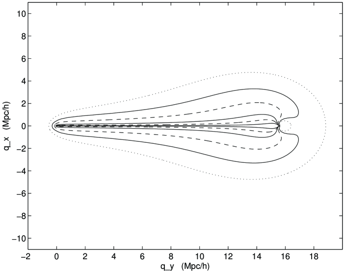
FIG. 1.: The comoving perimeter of the turn-around surface for the moving filament, with initial velocity $u_{i}=.2$ and CDM. The curves are for the redshifts $z=200$ (innermost contour), $50$, $20$, $5$, $3$, and $1$ (outermost contour). For $z<2.1$ the turn-around consists of two contours.

It is worth mentioning that the accretion is also suppressed (on small scales, $q_{x}\approx 0$) near ${\bf q}=(0,q_{i})$, as happens with the small scale suppression due to free streaming. This is shown in Figure 2 where the turn-around redshift is plotted as a function of $q_{x}$ for $q_{y}=q_{i}/2$, and for $q_{y}=q_{i}$ where such a suppression is observed (dotted line and continuous line). These curves look like the case of a static filament in HDM models[25], however, here the suppression at a fixed time $t\gg t_{i}$ occurs only on scales much smaller than the suppression caused by the free streaming. This is readily seen by rewriting equation (22) for $q_{y}=q_{i}$

$$q_{x}^{2}=q_{x,st}^{2}+b(t)\,ln\left(\frac{q_{x}^{2}}{q_{x}^{2}+q_{i}^{2}}\right)\,,$$ (23)

where $q_{x,st}$ is the turn-around comoving position (the $x$ component) in the case of a stationary filament. For small values of $|q_{x}|$, the $ln$ term on the right hand side of (23) contributes with a very large negative value (the $tan^{-1}$ terms are finite even for $q_{y}\neq q_{i}$), thereby implying that turn-around is possible in that region just for very large times (compared to $t_{i}$). This suppression is also a consequence of the peculiar motion of the string whose gravitational force on a cold dark particle acts in different (though correlated) directions at different times, which is not the case on large scales. Such a small scale suppression does not occur in the case of loops[21]. This can also be explained by taking into account the gravitational action of each defect.

Figure 2

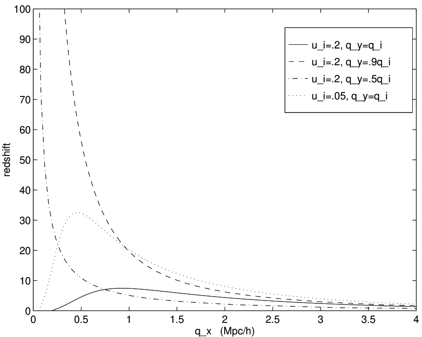
FIG. 2.: Redshift versus $q_{x}$ for different values of $q_{y}$ and $u_{i}$.

The overall effect of the string motion is to distort the cross-section of the turn-around surface (a circle in the stationary case). However, the suppression along the $x$ axis is more than compensated by the growth along the $y$ axis (see Figure 1). In fact, the suppression along $x$ is only logarithmic in the string velocity (it goes as $ln(1/q_{i})$) while the length of the wake along the $y$ axis increases linearly (proportional to $q_{i}$). In contrast, the total amount of CDM accreted by a string loop is independent of the velocity (see Refs. [26] and [21]). Figure 3 shows the dependence of the maximum value $q_{nl,x}(q_{y})$ as a function of the velocity of the seed.

Figure 3

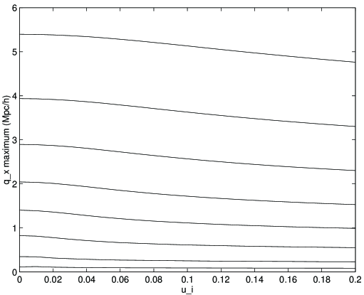
FIG. 3.: Variation of the maximum of $q_{nl,x}(q_{y})$ as a function of the velocity of the seed. The plots are for $z=1000$ (lowermost curve), $200$, $50$, $20$, $10$, $5$, $2.5$, and $1$ (uppermost curve). The difference for $q_{nl,x}(q_{y},u_{i})$ between $u_{i}=0$ and $u_{i}=.2$ falls from $25\%$ for $z=1000$ to $11\%$ for $z=1$.

We have calculated numerically the total nonlinear mass (i. e. the mass inside the turn-around surface) as a function of the redshift. A reasonable approximation can be obtained by assuming that the area inside the turn-around curve defined by (22) is given by

$$A=\pi Q_{CDM}^{2}+q_{i}\frac{l_{x}}{2}\,,$$ (24)

where $l_{x}$ is the the comoving width of the turn-around volume at its thickest point (near $q_{y}=q_{i}$). The second term in (24) corresponds to the area of an isosceles triangle whose base is $l_{x}$ and height is $q_{i}$. This equation in fact yields a lower limit for the total mass that has gone nonlinear. Since a lower bound to $\Omega_{nl}$ will be derived in Section 5, it is appropriate at this point to obtain a lower limit to the accreted mass.

The second term in (24) is proportional to $u_{i}$, the initial velocity of the string, whereas the first term in the limit $u_{i}=0$ reduces to the results of Ref. [25] for the static case. Comparing the two terms, we see that the second term in (24), stemming from the motion of the string, gives the dominant contribution if

$${{2\pi}\over{15u_{i}}}(\lambda G)_{6}^{1/2}(z(t)+1)^{-1/2}h\Omega^{1/2}<1,$$ (25)

where $(\lambda G)_{6}$ is the value of $\lambda G$ in units of $10^{-6}$. For example, we see that if $t_{i}=t_{eq}$, $(\lambda G)_{6}=0.5$, $h=1/2$, $\Omega=1$ and $u_{i}=0.2$, then the two terms are comparable at redshift 0, but the contribution originating from the second term in (24), the contribution specifically due to the motion of the string, dominates for higher redshifts.

The total mass accreted can be written as (see Equation (20))

$$M(z,u_{i})=\xi\rho_{0}t_{i}(z_{i}+1)A(z,u_{i})\,,$$ (26)

where $(z_{i}+1)=(t_{0}/t_{i})^{2/3}$ and $A(z,u_{i})$ is the area given by (24). As a consistency check, we note that taking the static limit ($q_{i}=0$) in the above equations, the results of Ref. [25] are readily recovered. For the values of the parameters used above, Equation (26) yields: $M\simeq 5\xi\times 10^{12}M_{\odot}A(z,u_{i})/Mpc^{2}$.

To proceed further, it proves convenient to summarize the main properties of the turn-around curve described by (22). For CDM we have checked numerically:

(i) The comoving area grows linearly with the scale factor (as a consequence of the fact that $ln(a/a_{i})$ is a slowly varying function of $a$) for $a\gg a_{i}$.

(ii) The area inside the turn-around curve grows almost linearly with the velocity of the filament $u_{i}$ for $u_{i}>.05$ and is practically constant for $u_{i}<.05$ at redshifts under consideration (because in the latter case the term in (24) independent of $u_{i}$ dominates).

(iii) Due to the motion of the filament, the accretion on large scales is strongly suppressed near the comoving initial position of the string (because the gravitational line source is far away for most of the time), whereas growth on small scales is suppressed at the end, when $q^{\prime}\sim q_{i}$.

(iv) Using $u_{i}=0.2$ and $t_{i}=t_{eq}$ we obtain at the redshift $z=4$ a turn-around curve whose length is $l\approx q_{i}\simeq 8h^{-2}Mpc$ and whose width in the thickest part $l_{x}$ is about $2h^{-1}(\lambda G)_{6}^{1/2}Mpc$. The area $A$ inside the curve is approximately $16h^{-3}(\lambda G)_{6}^{1/2}Mpc^{2}$ which corresponds to a mass per unit length of $M=\xi A\rho_{0}t_{eq}z_{eq}\simeq 50\xi\times 10^{12}h^{-1}(\lambda G)_{6}^{1/2}M_{\odot}$.

IV Accretion of Hot Dark Matter

Now we turn to the accretion of hot dark matter. The basic equations (13 - 20) which describe accretion onto a moving Newtonian line source are applicable.

We will deal with the ambiguity in the definition of $t_{s}(q)$ mentioned in Section 2 in the following way: Since we are only interested in the motion of dark matter in the direction perpendicular to the seed velocity, we may replace the initial condition (7) by

$$t_{s}=\frac{t_{0}\lambda_{0}^{3}}{|q_{x}|^{3}}\,.$$ (27)

This, however, seems to overestimate the free streaming effect, since it completely erases the accretion in the region near the initial location of the string (an improved analysis using the Boltzmann equation is in progress and will be reported elsewhere). In the following we will adopt (27) as a generalization of the condition used for static seeds which is a good approximation for the real free streaming effect [15]. The quantities we are going to obtain in this case, such as the total mass accreted, are lower bounds to the exact ones.

Since we must have $t_{s}\geq t_{i}$, condition (27) can be applied only if $|q_{x}|\leq v_{i}t_{i}(z_{i}+1)$, otherwise the condition $t_{s}=t_{i}$ is to be used even for HDM.

Thus, only a few small changes must be made: In the turn-around conditions we substitute $a_{s}=\frac{\lambda_{0}^{2}}{|q_{x}|^{2}}$. Then for HDM, equation (18) may be cast as

$$q_{x}^{2} + (q_{y}-q_{i})^{2}=Q_{CDM}^{2}+b(t)\left\{ln\left(\frac{q_{x}^{2}}{\lambda_{i}^{2}}\right)+ln\left(\frac{q_{x}^{2}+q_{y}^{2}}{q_{x}^{2}+(q_{y}-q_{s})^{2}}\right)\right.$$ (29)

$$\left.-2\frac{q_{y}-q_{i}}{q_{x}}\left[tan^{-1}\left(\frac{q_{y}-q_{s}}{q_{x}}\right)-tan^{-1}\left(\frac{q_{y}}{q_{x}}\right)\right]\right\}\,.$$

where $q_{s}=q_{i}(1-|q_{x}|/\lambda_{i})$, and $\lambda_{i}=\lambda_{0}/\sqrt{a_{i}}=\lambda_{J}(t_{i})$.

As shown in Figure 4, the turn-around curve (29) is composed of two identical disconnected closed curves, one for negative values of $q_{x}$ and the other for positive values of $q_{x}$. It is apparent from the figure that the nonlinearities on small scales are highly suppressed by the free streaming condition - see (7).

Figure 4

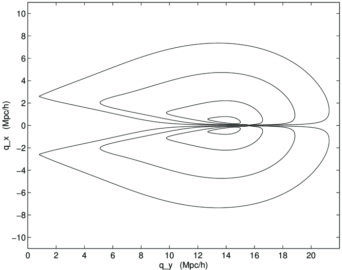
FIG. 4.: The same as Figure 1, but now for HDM with velocity $v_{eq}=.1$. Contours (two sheets each one) are drawn for $z=20$ (inner contour), $5$, $1$, and $0$ (outer contour).

In order to compare to other cases let us rewrite (29) for $q_{y}=q_{i}$

$$q_{x}^{2}=q_{x,CDM}^{2}+b(t)\left\{ln\left(\frac{q_{x}^{2}}{\lambda_{i}^{2}}\right)+ln\left(\frac{q_{x}^{2}+q_{i}^{2}}{q_{x}^{2}+q_{i}^{2}{|q_{x}|}{\lambda_{i}}^{-1}}\right)\right\}\,.$$ (30)

Recalling that equation (30) applies for $|q_{x}|\leq\lambda_{i}$ (for larger values of $|q_{x}|$ the CDM result is valid) we see that the first $ln$ term on the right hand side of (30) is negative while the second one is positive. At early times, when $q_{x}^{2}<<q_{i}^{2}$ those two terms reduce to $ln(|q_{x}|/\lambda_{i})$ and a numerical analysis shows that for $v_{i}\leq u_{i}$ the ratio of this term to $q_{x,CDM}^{2}$ is very small. This means that for a rapidly moving filament the suppression of the turn-around near $q_{y}=q_{i}$ is governed by the seed motion and is the same for both CDM and HDM. For $v_{i}>u_{i}$ the suppression due to the free streaming is important also for $q_{y}=q_{i}$. These features can be seen from Figures 2 and 5, graphs which plot the redshift corresponding to the onset of nonlinearity as a function of $q_{x}$ for different velocities of the string. For instance, for the value $u_{i}=0.2$, the curves for $q_{y}=q_{i}$ in the cases of CDM (Figure 2) and HDM (Figure 5) are essentially the same, whereas for the value $u_{i}=0.05$, the HDM curve is substantially lower at small values of $q_{x}$. Figure 5 also shows that there are no nonlinear structures for redshifts greater than about 90.

Figure 5

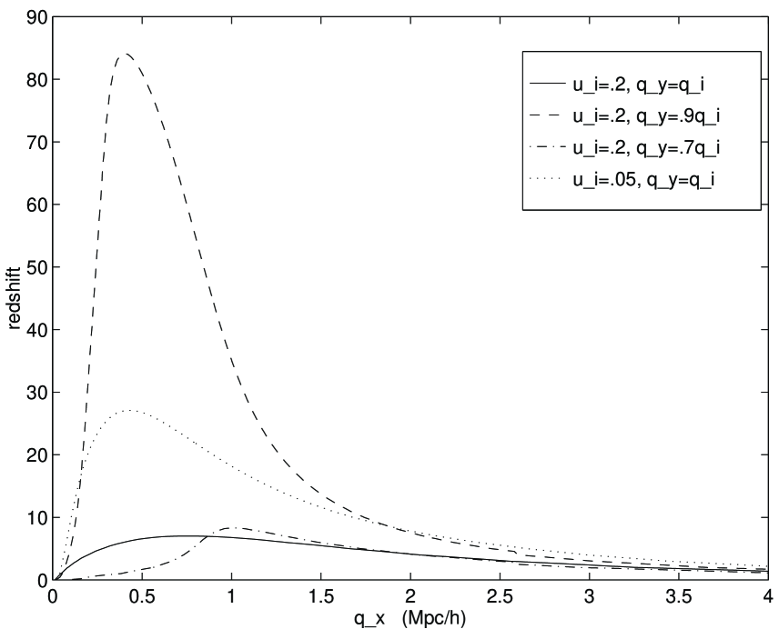
FIG. 5.: Same as figure 2, now for HDM with velocity $v_{eq}=.1$.

We know that free streaming completely erases the nonlinearities on scales smaller than the free streaming length. Equation (29) shows this behavior as a consequence of the term $ln(q_{x}^{2}/\lambda_{i}^{2})$, which is independent of $q_{y}$ and for small $|q_{x}|$ is highly negative implying that turn-around can only occur at late times. As we have seen in the previous section, for $q_{y}<q_{i}$ the $tan^{-1}$ terms are also important in determining the turn-around on large scales (they are finite even for $q_{x}\longrightarrow 0$). Then, the presence of the new $tan^{-1}$ term in (30) will not significantly change the results, and it follows that for a moving filament with HDM, the wake is strongly erased in the thinnest region near the starting position of the seed (see Figure 4).

The total nonlinear mass accreted in the HDM model can be estimated by considering all the mass inside and between the two disjoint curves (see Figure 4). We then approximate the turn-around curve by a trapezoid. Such a figure figure is obtained when the height $q_{i}$ of the isosceles triangle considered in the CDM case is reduced to $l_{y}$, thereby accounting for the free streaming suppression. By comparing Figures 1 and 4 it can be seen that the difference in the nonlinear mass between HDM and CDM is large at high redshift and decreases at later times. The length $l_{y}$ of the turn-around curve along the $y$ axis depends on the redshift and tends to $q_{i}$ for very late times (e.g. for $z<2$ if $t_{i}=t_{eq}$). According to Figure 4, a simple (underestimating) approximation is to take $l_{y}=q_{i}-q_{y}(\lambda_{i})$, where $q_{y}(\lambda_{i})$ is given by the intersection between the line $q_{x}=-\lambda_{i}q_{y}/q_{i}+\lambda_{i}$ and the approximated turn-around curve for CDM (see the comments below (24)). The result is $l_{y}=q_{i}-\lambda_{i}q_{i}/(\lambda_{i}+l_{x}/2)$. Hence, the area of the nonlinear region can be estimated as

$$A_{HDM}=\pi Q_{HDM}^{2}+q_{i}\frac{l_{x}}{2}\left(1-\frac{\lambda_{i}^{2}}{(\lambda_{i}+l_{x}/2)^{2}}\right)\,,$$ (31)

where $Q_{HDM}^{2}$ stands for the right hand side of (30). The first term is analogous to the one introduced in the CDM case, the first term in equation (24), which represents the accretion onto a static filament (at the comoving position $q_{i}$) with HDM. For $t$ sufficiently greater than $t_{i}$ the second term in (31) dominates if the same condition for CDM, Equation (25), is satisfied. In such a case we can parameterize the result as follows:

$$M_{HDM}(t,t_{i},u_{i})=f(t,t_{i},u_{i})M_{CDM}(t,t_{i},u_{i}),$$ (32)

where $f(t,t_{i},u_{i})$ is the function which parameterizes the mass suppression in the case of HDM. For large $t$, the result with HDM asymptotically approaches the CDM result. Hence

$$lim_{t\rightarrow\infty}f(t,t_{i},u_{i})=1.$$ (33)

The numerical analysis shows that for the cosmological and cosmic string parameters used (see Section 3), at a redshift of $z=10$, $f(t,t_{eq},u_{i})\approx 0.5$, and for $z=4$, $f(t,t_{eq},u_{i})\approx 0.8$. The function $f(t,t_{i},u_{i})=1-\frac{\lambda_{i}^{2}}{(\lambda_{i}+l_{x}/2)^{2}}$ used in (31) furnishes the following approximate values: $f=0.5$, $f=0.85$, and $f=0.96$ respectively for $z=10$, $z=4$ and $z=0$. We have taken $l_{x}=2|q_{x}|$ with $q_{x}$ given by (24) (see following discussion).

V The Nonlinear Density Parameter $\Omega_{{n}{l}}$

To illustrate the results of the previous sections, let us now compute the fraction $\Omega_{nl}$ of the critical density accreted onto filaments both for CDM and HDM models. Naturally, by considering only the accretion onto filamentary structures we will be underestimating the total contribution to $\Omega_{nl}$ due to the cosmic string network. Let us first consider the case where the initial string velocities $u_{i}$ and times $t$ are such that the second term in (24), the term specific to the motion of the string, dominates. This is the case of primary interest to us, since in the other limit($q_{i}=0$) the results for static filaments are recovered (see eqs.(20) and (26)).

As argued earlier (see Section 3), to estimate $\Omega_{nl}$ in the case of moving filaments with CDM, one may approximate the turn-around curve by an isosceles triangle whose height and base are respectively $l_{y}=q_{i}$ and $l_{x}$, where $l_{x}$ is the width of the thickest region of the wake. A good approximation for the width is $2|q_{x}|$, where $q_{x}$ is given by (23) without the term $ln[q_{x}^{2}/(q_{x}^{2}+q_{i}^{2})]$. This term leads to a suppression of small scales, whereas for large scales it is small in comparison to $ln(a/a_{i})$. In this way, by considering the mass of the wake for $0\leq q_{y}\leq q_{i}$, such a term may be safely neglected. The resulting expression for $q_{x}$ is then the same as for a static filament located at $q_{i}$ since the initial time $t_{i}$. Also, the condition that the string is not near $q_{i}$ for all times after $t_{i}$, can be effectively described replacing $t_{i}$ by the rescaled time $t_{eff}=\alpha t_{i}$, where $0<\alpha\leq 1$. The time $t_{eff}$ can be thought as a sort of initial time for which the Newtonian line starts to act effectively as a static source for accretion near $q_{i}$. The value of $\alpha$ may be fixed by comparing the exact value of $q_{x}$ obtained numerically with the approximation given by $q_{x,static}(t,\alpha t_{i})$. As can be easily seen, for the values of the parameters considered here one has $\alpha\approx 10^{-1}$. In the limit $\alpha\rightarrow 1$, the relative error for sufficiently large times may be written as $ln(\alpha)/ln(t/t_{i})$, and for $t_{i}=t_{eq}$, it is about $15\%$ at the present time (see Figure 3 for comparison).

The total mass accreted onto the filament during an arbitrary time interval $\Delta t=t-t_{i}$ ($t_{i}\leq t\leq t_{o}$), is the mass contained in the Lagrangian volume inside the turn-around surface. Since the length of the turn-around tube is proportional to the Hubble radius at time $t_{i}$, the accreted mass is given by (see Section 3)

$$M(t,t_{i})=\xi\frac{u_{i}}{2\pi}\sqrt{\frac{18\lambda}{5G}}t_{i}\left(\frac{t}{t_{i}}\right)^{1/3}\sqrt{ln\left(\frac{t}{t_{i}}\right)+\frac{3}{20}}\,.$$ (34)

This is the total mass that has gone nonlinear at time $t>t_{i}$ onto a Newtonian line formed at time $t_{i}$. Note that the nonlinear mass grows as $t^{1/3}$ and not as $t^{2/3}$ as in the linear theory for static seeds. The difference comes from the fact that the length along the direction of string motion depends only on the velocity of the seed, and is, to the first order of approximation, time independent. As expected, for slowly moving strings, the first term in (24) dominates, and the usual linear perturbation theory growth of the total nonlinear mass is recovered. This can also be seen by using (25) to determine the lower cutoff velocity when (34) is applicable, and substituting in (34) for the velocity $u_{i}$. This yields the extra factor of $(z(t)+1)^{-1/2}$.

From the scaling solution of the string network we know that the number of long strings per physical volume at time $t$ created in the interval between $t_{i}$ and $t_{i}+dt_{i}$ assume the form

$$n(t,t_{i})dt_{i}=\frac{\tilde{\nu}}{t_{i}^{2}t^{2}}dt_{i}\,,$$ (35)

where $\tilde{\nu}$ is a constant which gives the number of long string segments passing through a volume $t^{3}$ at any given time (this number is independent of time as a consequence of string scaling). Using this number density we obtain the fraction of the critical density of objects formed by accretion of CDM onto moving filaments in the interval between $t_{eq}$ and $t$ as

$$\Omega_{nl}(t)=6\pi Gt^{2}\int_{t_{eq}}^{t}{n(t,t_{i})M(t,t_{i})dt_{i}}\,,$$ (36)

where $M(t,t_{i})$ is given by (34).

Then by direct integration of (36) we obtain to a first approximation

$$\Omega_{nl}(t) \approx 9\xi\tilde{\nu}u_{i}\sqrt{\frac{18\lambda G}{5}}\sqrt{\ln\left(\frac{t}{t_{eq}}\right)}\left(\frac{t}{t_{eq}}\right)^{1/3}$$ (38)

$$\approx 2\xi\tilde{\nu}(u_{i})_{0.2}(\lambda G)_{6}^{1/2}h(z(t)+1)^{-1/2}\,,$$

where $(u_{i})_{0.2}$ is the value of $u_{i}$ in units of $0.2$. It follows that for $u_{i}=0.2$ and $(\lambda G)_{6}=0.5$ the value of $\Omega_{nl}(t_{0})$ at the present time $t_{0}$ is about $2\xi\tilde{\nu}$. Note that the above result is valid for values of $u_{i}$ for which (25) is satisfied. For smaller initial string velocities, by solving (25) for $u_{i}$ and inserting in (38)), we obtain in the static limit

$$\Omega_{nl,st}(t)=\frac{18}{5}\pi\lambda G\tilde{\nu}\left(\frac{t}{t_{eq}}\right)^{2/3}ln\left(\frac{t}{t_{eq}}\right)\approx\xi\tilde{\nu}{{2\pi}\over 3}(\lambda G)_{6}(z(t)+1)^{-1}h^{2}\,.$$ (39)

For HDM we have approximated the turn-around curve by a trapezoid (see the discussion below equation (30)). The velocity depending area $A_{HDM}$ inside such a curve is given by

$$A_{HDM}=f(t,t_{i},u_{i})A_{CDM}=q_{i}\frac{l_{x}}{2}\left(1-\frac{\lambda_{i}^{2}}{(\lambda_{i}+l_{x}/2)^{2}}\right)\,,$$ (40)

As mentioned before, this area includes the holes inside and between the curves of Figure 4. This means that all $ln$ terms in (30) are neglected. As a matter of fact, the suppression terms due to free streaming are important only for small scales which have been by the above approximation included in $A_{HDM}$. Besides, the term in (30) arising from the motion of the string may also be neglected by the same reason as discussed earlier. As a consequence, the expression of $q_{x}$ for HDM reduces to the same one derived in the CDM model.

The value of $\Omega_{nl}$ in the case of HDM can be estimated by following (36):

$$\Omega_{nl}^{HDM}=6\pi Gt^{2}\int_{t_{eq}}^{t}n(t,t_{i})f(t,t_{i},u_{i})M_{CDM}(t,t_{i},u_{i})dt_{i}\,.$$ (41)

Since the integral is dominated at the lower end, we can approximate the result as

$$\Omega_{nl}^{HDM}(t) \simeq f(t,t_{eq},u_{i})\Omega_{nl}^{CDM}(t)\,$$ (43)

$$\simeq\left(1-\frac{\lambda_{eq}^{2}}{[\lambda_{eq}+l_{x}(t,t_{eq})/2]^{2}}\right)\Omega_{nl}^{CDM}\,,$$

where, as we have seen above, $f(t,t_{eq},u_{i})$ grows from $f\simeq 0$ at $t=t_{eq}$ to $f\simeq 0.96$ at $t=t_{0}$.

For the sake of completeness, let us now write the contributions from the first terms in equations (24) and (31) to the fraction of nonlinear mass. As discussed earlier, these terms correspond to the fraction of the accreted mass onto static filaments. Following the previous procedure we get

$$\Omega_{nl,st}^{CDM}\simeq\frac{18}{5}\pi\xi\tilde{\nu}\lambda G\left(\frac{t}{\alpha t_{eq}}\right)^{2/3}ln\left(\frac{t}{\alpha t_{eq}}\right)\,,$$ (44)

(compare with (39)) and for HDM

$$\Omega_{nl,st}^{HDM}\simeq(1-\chi)\Omega_{nl,st}^{CDM}\,,$$ (45)

where $1-\chi$ is the suppression factor due to free streaming. $\chi=\chi(t,t_{eq})$ falls from $\chi=1$ for $t=t_{eq}$ to $\chi\approx 0$ at $t=t_{0}$. Notice that $\Omega_{nl,st}$ varies with $(z+1)^{-1}$ while the contribution due to the string motion, equations (38) and (43), goes as $(z+1)^{-1/2}$. This fact explains why $\Omega_{nl,st}$ is important just for small $z$, when compared to the terms depending on the seed velocity.

These results show that even with hot dark matter (given the string parameters used above), accretion onto filaments can easily lead to $\Omega_{nl}=1$ at the present time.

VI Conclusions

We have studied the accretion of hot and cold dark matter onto moving gravitational line sources and applied the results to the cosmic string filament model of structure formation. Our main result is that even for initial relativistic motion of the strings, nonlinear structures can develop at redshifts close to 100 if the dark matter is hot (a point not realized in earlier work [11]). Thus, string filaments are much more efficient at clustering hot dark matter at early times than string wakes.

The total fraction $\Omega_{nl}$ of nonlinear mass depends quite sensitively on the string parameters used, i.e. on the initial string velocity $u_{i}$, on the strength $\lambda G$ of the Newtonian potential, and on the values of the constants $\xi$ and $\tilde{\nu}$ which determine the curvature radius and number of strings in the scaling solution. However, the uncertainties partially cancel. For example, the product $\tilde{\nu}\xi$ is a measure of the total mass density in strings and can in principle be determined from numerical simulations of cosmic string evolution. Also, as $\lambda G$ increases, the value of $u_{i}$ will decrease, but in this case the cancelation is only partial since $u_{i}$ cannot exceed 1 and hence in the limit $\lambda G\rightarrow 0$ the filamentary accretion will disappear (and the only effect of the strings will be the wakes caused by the velocity perturbations).

According to the numerical simulations of Allen and Shellard [6] (which, however, are based on strings obeying the Nambu-Goto action and hence not directly applicable to strings with a large amount of small-scale structure), the value of $\xi\tilde{\nu}$ is about 15 in the radiation dominated epoch and slightly less during matter domination. Taking the value $(\lambda G)_{6}=0.5$ which corresponds to the largest possible effect of small-scale structure for GUT scale strings, we find that even for hot dark matter, all of the mass in the Universe has gone nonlinear by a redshift of about 5. This implies that the cosmic string model - provided the small-scale structure dominates - is easily compatible with the cosmological constraints from both high redshift quasar [27] and damped Lyman alpha system [28] abundances.

It is interesting to compare the results derived here with those from the cosmic string wake [15] and loop [22] scenarios. If the dark matter is hot, wakes do not produce any nonlinearities until a redshift of close to 1. Loops do produce nonlinear objects at high redshifts, but objects of mass $10^{12}M_{\odot}$ only form at a redshift of about 4. Hence, we conclude that string filaments are the most efficient way of forming high redshift massive nonlinear structures in the cosmic string model. Unfortunately, it is not known how much small-scale structure cosmic strings are endowed with. The cosmic string evolution simulations at present do not have the required range to resolve this issue, and analytical analyses are needed to address this question. In light of the sensitive dependence of high redshift structure formation to the amount of small-scale structure, it is crucial to improve our understanding of the small-scale structure on strings.

Acknowledgments

The authors are grateful to R. Moessner and M. Parry for useful discussions. This work is supported in part by the Conselho Nacional de Desenvolvimento Científico e Tecnológico- CNPQ(Brazilian Research Agency), and by the US Department of Energy under contract DE-FG0291ER40688, Task A .

REFERENCES

-
[1]
A. Vilenkin and E.P.S. Shellard, Cosmic strings and
other topological defects (Cambridge Univ. Press, Cambridge, 1994);
M. Hindmarsh and T.W.B. Kibble, Rept. Prog. Phys. 58, 477 (1995);
R. Brandenberger, Int. J. Mod. Phys. A9, 2117 (1994). -
[2]
Ya. B. Zeldovich, Mon. Not. R. astr. Soc. 192, 663
(1980);
A. Vilenkin, Phys. Rev. Lett. 46, 1169 (1981). -
[3]
D. Bennett, A. Stebbins and F. Bouchet, Ap. J.
(Lett.) 399, L5 (1992);
L. Perivolaropoulos, Phys. Lett. B298, 305 (1993). - [4] T.W.B. Kibble, J. Phys. A9, 1387 (1976).
- [5] A. Vilenkin, Phys. Rept. 121, 263 (1985).
-
[6]
D. Bennett and F. Bouchet, Phys. Rev. Lett. 60,
257 (1988);
B. Allen and E.P.S. Shellard, Phys. Rev. Lett. 64, 119 (1990);
A. Albrecht and N. Turok, Phys. Rev. D40, 973 (1989). -
[7]
A. Vilenkin, Phys. Rev. D23, 852 (1981);
J. Gott, Ap. J. 288, 422 (1985);
W. Hiscock, Phys. Rev. D31, 3288 (1985);
B. Linet, Gen. Rel. Grav. 17, 1109 (1985);
D. Garfinkle, Phys. Rev. D32, 1323 (1985);
R. Gregory, Phys. Rev. Lett. 59, 740 (1987). - [8] B. Carter, Phys. Rev. D41, 3869 (1990).
- [9] J. Silk and A. Vilenkin, Phys. Rev. Lett. 53, 1700 (1984).
- [10] T. Vachaspati, Phys. Rev. Lett. 57, 1655 (1986).
- [11] T. Vachaspati and A. Vilenkin, Phys. Rev. Lett. 67, 1057 (1991).
- [12] T. Vachaspati, Phys. Rev. D45, 3487 (1992).
- [13] D. Vollick, Phys. Rev. D45, 1884 (1992).
- [14] Ya. B. Zeldovich, Astr. Astrophys. 5, 84 (1970).
-
[15]
L. Perivolaropoulos, R. Brandenberger and A. Stebbins, Phys. Rev. D41, 1764 (1990);
R. Brandenberger, L. Perivolaropoulos and A. Stebbins, Int. J. Mod. Phys. A5, 1633 (1990);
R. Brandenberger, Phys. Scripta T36, 114 (1991). -
[16]
N. Turok and R. Brandenberger, Phys. Rev. D33, 2175
(1986);
H. Sato, Prog. Theor. Phys. 75, 1342 (1986);
A. Stebbins, Ap. J. (Lett.) 303, L21 (1986). -
[17]
R. Brandenberger, N. Kaiser, D. Schramm and N. Turok, Phys. Rev. Lett. 59, 2371 (1987);
R. Brandenberger, N. Kaiser and N. Turok, Phys. Rev. D36, 2242 (1987). - [18] A. Vilenkin and Q. Shafi, Phys. Rev. Lett. 51, 1716 (1983).
- [19] E. Bertschinger and P. Watts, Ap. J. 328, 23 (1988).
- [20] R. Scherrer, A. Melott and E. Bertschinger, Phys. Rev. Lett. 62, 379 (1989).
- [21] E. Bertschinger, Ap. J. 316, 489 (1987).
- [22] R. Moessner and R. Brandenberger, Mon. Not. R. astr. Soc. 280, 797 (1996).
- [23] A. Stebbins, S. Veeraraghavan, R. Brandenberger, J. Silk and N. Turok, Ap. J. 322, 1 (1987).
- [24] D. Vollick, Ap. J. 397, 14 (1992).
- [25] A. Aguirre and R. Brandenberger, Int. J. Mod. Phys. D4, 711 (1995).
- [26] M. Rees, Mon. Not. R. astr. Soc. 222, 23 (1986).
-
[27]
S. Warren, P. Hewett and P. Osmer, Ap. J. (Suppl.) 76, 23 (1991);
M. Irwin, J. McMahon and S. Hazard, in ‘The space distribution of quasars’, ed. D. Crampton (ASP, San Francisco, 1991), p. 117;
M. Schmidt, D. Schneider and J. Gunn, ibid., p. 109;
B. Boyle et al., ibid., p. 191;
M. Schmidt, D. Schneider and J. Gunn, Astron. J. 110, 68 (1995). -
[28]
K. Lanzetta et al., Ap. J. (Suppl.) 77, 1 (1991);
K. Lanzetta, D. Turnshek and A. Wolfe, Ap. J. (Suppl.) 84, 1 (1993);
K. Lanzetta, A. Wolfe and D. Turnshek, Ap. J. 440, 435 (1995).