High resolution spectroscopy of the line emission from the inner circumstellar ring of SN 1987A and its hot spots

We discuss high resolution VLT/UVES observations (FWHM $\sim 6\rm\leavevmode\nobreak\ km\leavevmode\nobreak\ s^{-1}$) from October 2002 (day $\sim 5700$ past explosion) of the shock interaction of SN 1987A and its circumstellar ring. A nebular analysis of the narrow lines from the unshocked gas indicates gas densities of $(\sim 1.5-5.0)\times 10^{3}\mbox{ cm}^{-3}$ and temperatures of $\sim 6.5\times 10^{3}-2.4\times 10^{4}$ K. This is consistent with the thermal widths of the lines. From the shocked component we observe a large range of ionization stages from neutral lines to [Fe XIV]. From a nebular analysis we find that the density in the low ionization region is $4\times 10^{6}-10^{7}\mbox{ cm}^{-3}$. There is a clear difference in the high velocity extension of the low ionization lines and that of lines from [Fe X-XIV], with the latter extending up to $\sim-390\rm\leavevmode\nobreak\ km\leavevmode\nobreak\ s^{-1}$ in the blue wing for [Fe XIV], while the low ionization lines extend to typically $\sim-260\rm\leavevmode\nobreak\ km\leavevmode\nobreak\ s^{-1}$. For H$\alpha$ a faint extension up to $\sim-450\rm\leavevmode\nobreak\ km\leavevmode\nobreak\ s^{-1}$ can be seen probably arising from a small fraction of shocked high density clumps. We discuss these observations in the context of radiative shock models, which are qualitatively consistent with the observations. A fraction of the high ionization lines may originate in gas which has yet not had time to cool down, explaining the difference in width between the low and high ionization lines. The maximum shock velocities seen in the optical lines are $\sim 510\rm\leavevmode\nobreak\ km\leavevmode\nobreak\ s^{-1}$. We expect the maximum width of especially the low ionization lines to increase with time.

1 Introduction

The core-collapse supernova (SN) 1987A in the Large Magellanic Cloud (LMC) is much closer to us than the SNe we normally observe. Detailed studies of SN 1987A have therefore contributed tremendously to our understanding of this type of SNe. Its interaction with circumstellar gas has also contributed to our understanding of shockwave physics (see e.g. Chevalier 1997; McCray 2005).

The radioactive debris of SN 1987A is at the center of a triple ring system where the two outermost rings are about three times the size of the innermost ring (Wang & Wampler 1992). The rings are elliptical in shape with the inner ring centered around the SN and the two outer rings are centered to the north and south of the SN forming a possible hour-glass structure. Since the inner ring (henceforth called the equatorial ring, or just ER) appears to be intrinsically close to circular in shape (Gould & Uza 1998; Sugerman et al. 2005), its observed ellipticity is interpreted as a tilt angle to the line of sight of $\sim 44^{\circ}$ (Plait et al. 1995; Burrows et al. 1995; Sugerman et al. 2002). How all the rings were formed is still unknown, but it seems clear that the ER is the result of the final blue supergiant wind interacting with previously emitted gas in the form of an asymmetric wind-like structure (e.g., Blondin & Lundqvist 1993; Chevalier & Dwarkadas 1995). In the models by Morris & Podsiadlowski (2005) the strong asymmetry is explained in a merger scenario being due to a rotationally enforced outflow. In these models also the outer rings may be explained by the merger, and the rings are likely to have been formed during the last $\sim$20,000 years before the explosion. Many details in both the observations and models are, however, uncertain.

The observed ER was photoionized to a high state of ionization by the SN flash accompanying the SN breakout (Fransson & Lundqvist 1989). It has since the breakout been cooling and recombining, giving rise to a multitude of narrow emission lines (e.g., Lundqvist & Fransson 1996). Already early it was realized that the ER should be reionized $\sim 10-20$ years after the explosion when the expanding SN ejecta would start to interact with the ER (Luo & McCray 1991; Luo et al. 1994). This event would cause a rebrightening of the ring and the first indication of this interaction became visible as a bright spot (Spot 1) in 1997 on the north side of the ring at PA = $29^{\circ}$ (Garnavich, Kirshner & Challis 1997; Sonneborn et al. 1998).

Modelling of Spot 1 (Michael et al. 2000) suggests that it is an inward protrusion of the dense ($\sim 10^{4}\mbox{ cm}^{-3}$, Lundqvist & Fransson 1996) ER and that it is embedded in the lower density ($\sim 10^{2}\mbox{ cm}^{-3}$, Chevalier & Dwarkadas 1995; Lundqvist 1999) H II region interior to the ring. The shocked gas drives a forward shock into this H II region and the bright Spot 1 is the result of the interaction of the shock and an inward protrusion of the inner circumstellar ring. When this happened, slower radiative shocks were transmitted into the protrusion and the radiation from these shocks appeared as a bright spot.

The velocities of the transmitted shocks are given by $V_{s}\sim V_{b}(n_{\rm HII}/n_{\rm sp})^{\frac{1}{2}}$, where $V_{b}$ is the blast wave velocity and $n_{\rm HII}$ and $n_{\rm sp}$ are the densities of the H II region and the protrusion, respectively. The fastest transmitted shocks are expected for head-on collisions, while slower velocities occur for tangential shocks. The shock velocities therefore depend on both the density and geometry of the spot. As a consequence, the transmitted shocks will have a wide range of velocities ($\sim 10^{2}-10^{3}\rm\leavevmode\nobreak\ km\leavevmode\nobreak\ s^{-1}$). However, only a fraction of these shocks will contribute to the observed UV/optical emission from the spot (Pun et al. 2002).

Since 1997 an increasing number of bright spots have been observed in the ER (Sugerman et al. 2002). This has marked the transition between the SN state and the SN remnant state, and for the first time we have the opportunity to study such a transition. A central issue for understanding the physics of the interaction is the hydrodynamics and physical conditions of the shocked region. High spectral resolution in combination with good spatial resolution is here invaluable. To address these issues we present in this paper high resolution optical spectroscopic VLT/UVES data, taken at 2002 October 4$-$7 (days 5702$-$5705). In a previous paper we have discussed some special aspects of these data, in particular the presence of a number of coronal lines from [Fe X-XIV] (Gröningsson et al. 2006). Here we discuss the observational analysis in greater detail, and in particular we concentrate on an analysis of lines from the low and medium ionization stages, as well as the narrow line component. In a forthcoming paper we will discuss the time evolution of the line emission using data from several epochs.

In Sect. 2 we discuss the observations and data reductions. In Sect. 3 we describe how to separate out emission lines both from different regions such as unshocked and shocked gas and different spatial positions of the ER. The analysis of these data is done in Sect. 4 where we also describe what conclusions can be drawn from the line profiles and nebular analysis. The results are discussed and summarized in Sect. 5.

2 Observations

Service mode observations of supernova remnant (SNR) 1987A were obtained on 2002 October 4$-$7 using the cross-dispersed Ultraviolet and Visual Echelle Spectrograph (UVES) at the ESO Very Large Telescope at Paranal, Chile. Details of the observations are given in Table LABEL:tab:obslog. The spectrograph separates the light beam into two different arms. One arm covering the shorter wavelengths ($3030-4990\mbox{ \AA}$) has a CCD detector with a spatial resolution of $0\aas@@fstack{\prime\prime}246$/pix. The arm covering the longer wavelengths ($4760-10\,600\mbox{ \AA}$) has two CCDs with spatial resolutions of $0\aas@@fstack{\prime\prime}182$/pix. The UVES spectrograph was used with two different dichroic settings and hence covering in total the wavelength range between $3030-10\,600\mbox{ \AA}$ with gaps at $5770-5830\mbox{ \AA}$ and $8540-8650\mbox{ \AA}$.

To encapsulate Spot 1 and to minimize the influence from the bright nearby stars a $0\aas@@fstack{\prime\prime}8$ wide slit was centered on the SN and rotated to PA = $30^{\circ}$. For these reasons and to be able to separate the north and south parts of the ER we requested an atmospheric seeing better than $0\aas@@fstack{\prime\prime}8$ for the observations (see Fig. 1). Since there are no real point sources inside the slit it is difficult to get a direct measure of the image quality from the data. Instead we chose to use the DIMM as an estimate. It typically overestimates the actual seeing by $\sim 0\aas@@fstack{\prime\prime}15$ but can serve as an upper limit. From Table LABEL:tab:obslog we see that the average DIMM seeing for these observations was $\sim 0\aas@@fstack{\prime\prime}8$. After a careful check we concluded that the data taken also at somewhat poorer DIMM seeing were good enough for our purposes, which are mainly to separate the north and south parts of the ER. (See also Appendix 1 for a discussion on the influence of seeing.)

For the slit width used for these observations the resolving power is $\sim 50\,000$, which corresponds to a spectral resolution of $\sim 6\rm\leavevmode\nobreak\ km\leavevmode\nobreak\ s^{-1}$.

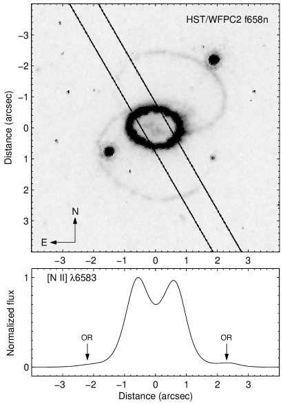
Figure 1: Upper panel: HST/WFPC2 [N II] $\lambda$6583 image of the triple ring system of SN 1987A from 2002 May 10. Overlaid is the slit position of our VLT/UVES observations (PA $=30^{\circ}$) from 2002 October. The slit width is $0\aas@@fstack{\prime\prime}8$ and the image size $8\aas@@fstack{\prime\prime}0\times 8\aas@@fstack{\prime\prime}0$. Lower panel: Flux of [N II] $\lambda$6583 along the slit in our 2002 October spectrum. The north (left) and south (right) parts of the inner ring result in two prominent peaks. Note also the two outer ring components (marked by “OR”) on either side of the inner ring.

2.1 Data reduction

The calibration data, according to the UVES calibration plan, include bias, wavelength calibration spectra, flat fields and spectrophotometric standard stars. Using the UVES pipeline version 2.0 as implemented in MIDAS, we produced the calibration sets needed for bias subtraction, flat-fielding, order extraction and wavelength calibration of the science data.

In order to produce reduced wavelength calibrated 2D spectra, the UVES pipeline command REDUCE/SPAT was used. The orders of the reduced and calibrated 2D spectra suffer from high noise levels near their ends, and especially so at the blue end. Moreover, by comparing consecutive orders of standard stars, we found that the flux levels at the overlapping regions differed significantly from each other. That could of course affect the relative fluxes of lines located near the ends of the orders. Since the automatic merging of the orders within REDUCE/SPAT did not give satisfactory results we chose to do the merging outside the pipeline. We first excluded both ends of each order and then applied a linear weighted averaging between the remaining overlapping regions for every order of the 2D frames before merging them. The overlap after cutting the ends of the orders were $\sim 10\mbox{ \AA}$ except for reddest part of the spectrum where the overlap was too small for making adequate mergings. Hence, those regions were removed from the final 1D spectrum (see Fig. 3) The accuracy in the wavelength calibration for the merged 2D spectra was checked against strong night sky emission lines and the systematic error was found to be $\sim 0.01\mbox{ \AA}$ over the whole spectral range, which is also guaranteed by the UVES team. In order to transform the wavelength calibrated data to a heliocentric frame we used the task RVCORRECT within the IRAF package to calculate the radial velocity component of the instrument with respect to SN 1987A due to the motion of the earth.

In addition to the sky emission lines the resulting 2D spectra show strong background emission from the LMC. In order to remove this source we used the IRAF routine BACKGROUND. We concluded that a simple linear interpolation could not sufficiently reduce the LMC background. Instead we chose a second order Legendre polynomial interpolation as an estimate of the background level. This interpolation proved to be a good estimate for the background emission in most cases. However, for [O II] and [O III] where the background is strong, the procedure was not able to remove all the background emission and some background artifacts in form of weak emission features may still remain after the subtraction. Nevertheless, since the background emission component has a different systemic velocity than the SN most of it is spectrally resolved from the ring emission, and does not significantly affect our results.

To extract 1D spectra from the 2D spectra we fitted the double peaked spatial profile (see Fig. 1) with the sum of two Gaussians. For the best fit, i.e. the least-square solution, each Gaussian represents one part of the ER i.e. north or south. The two-gaussian model was then extracted in the dispersion direction. The resulting 1D spectra were average-combined with weights proportional to their exposure times. Within this process we applied a sigma clipping routine which effectively rejected outliers of the data such as cosmic rays which heavily contaminated the individual spectra.

The flux calibration of the data was performed by using the UVES master response curves and the atmospheric extinction curve provided by ESO. Different response curves for different standard settings and epochs are provided. To check the quality of the flux calibration we reduced the spectrophotometric standard star spectra with the same calibration sets as for the science spectra. The width of the slit used for the standard star observations was $10\aas@@fstack{\prime\prime}0$ and slit losses should therefore be negligible. The extracted flux-calibrated standard-star spectra was compared to their tabulated physical fluxes. The fluxes obtained by using the master response curves showed to be accurate to $\sim 10\%$ in level and shape in general. The science spectra were corrected for this discrepancy.

The data were observed with an atmospheric dispersion corrector and thus we consider the slit losses to be close to monochromatic. However, another source of uncertainties could be due to possible misalignment of the relatively narrow slit ($0\aas@@fstack{\prime\prime}8$) for the science observations which could cause substantial losses in flux. Investigations by eye of the slit images, provided as a part of the UVES calibration plan, revealed that the slit was accurately placed across the SN. Nevertheless, flux losses are still, of course, seeing dependent. To estimate how sensitive fluxes are to different seeing conditions we compared various line fluxes of the individual science exposures and concluded that the fluxes differ by $\!\!\!\phantom{\leq}\smash{\buildrel\over{\lower 2.67502pt\hbox{$\buildrel\lower 2.14001pt\hbox{$\displaystyle<$}\over{\sim}$}}}\,\,10\%$ between the different exposures. From these measurements, and the results in Appendix 1 where we have compared our UVES fluxes to data taken with the Hubble Space Telescope at similar epochs, we are confident that the systematic error of the absolute flux should be less than $20-30$%. As discussed above, the relative fluxes should, however, be accurate to $\sim 10-15$%.

To create the final spectrum the combined spectra from all settings were merged by applying a linearly weighted averaging between the overlapping regions for the settings.

Table 1: VLT/UVES observations of SN 1987A and its rings at days 5702$-$5705 past explosion. The airmasses of these observations were $\sim 1.5$.

Date	Grating Setting	Wavelength Range	Slit	Seeing	Exposure time
		(nm)	(arcsec)	(arcsec)	(s)
2002-10-04	CD#4 860	660 - 1060	$12.0\times 0.8$	$0.91\pm 0.06$	3600
2002-10-04	CD#2 437	373 - 499	$10.0\times 0.8$	$0.91\pm 0.06$	3600
2002-10-04	CD#2 437	373 - 499	$10.0\times 0.8$	$1.05\pm 0.20$	2160
2002-10-04	CD#4 860	660 - 1060	$12.0\times 0.8$	$1.05\pm 0.20$	2160
2002-10-05	CD#4 860	660 - 1060	$12.0\times 0.8$	$0.44\pm 0.05$	3600
2002-10-05	CD#2 437	373 - 499	$10.0\times 0.8$	$0.44\pm 0.05$	3600
2002-10-06	CD#3 580	476 - 684	$12.0\times 0.8$	$0.99\pm 0.13$	3600
2002-10-06	CD#1 346	303 - 388	$10.0\times 0.8$	$0.99\pm 0.13$	3600
2002-10-06	CD#3 580	476 - 684	$12.0\times 0.8$	$0.94\pm 0.18$	3600
2002-10-06	CD#1 346	303 - 388	$10.0\times 0.8$	$0.94\pm 0.18$	3600
2002-10-07	CD#1 346	303 - 388	$10.0\times 0.8$	$0.65\pm 0.05$	3000
2002-10-07	CD#3 580	476 - 684	$12.0\times 0.8$	$0.65\pm 0.05$	3000

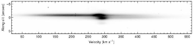
Figure 2: The 2D background subtracted spectrum from 2002 October 6 showing H$\alpha$. The vertical direction of the plot is along the slit, with the northern part in the upward direction. The total spatial extent is 12 arcsec. The velocities are with respect to the rest wavelength of H$\alpha$. Note how the two intersections of the slit with the ER and the outer rings are clearly visible around the rest velocity of the supernova, as well as the weaker emission from the outer rings. The broader (few$\times 10^{2}\rm\leavevmode\nobreak\ km\leavevmode\nobreak\ s^{-1}$) emission (the “intermediate” component) is asymmetric, with the blue side dominating for the northern ER, and the red side for the southern ER.

3 Results

From our data we were able to spatially separate the northern and the southern parts of the ER in the reduced 2D frames (see Fig. 2) to extract 1D spectra. Figure 3 shows the full spectrum from the northern part of the ring, with a number of the stronger lines marked.

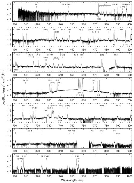
Figure 3: Extracted 1D spectrum from the northern part of the ER. The most significant/important lines are marked. The gaps in the reddest part of the spectrum (lowest panel) are due to the poor overlapping in wavelength between different orders. Many of the lines show both narrow and intermediate components (cf. Tables LABEL:tab:narrowlines–LABEL:tab:broadlinesS). Note also the very broad H$\alpha$ emission component (the middle panel) originating from the ejecta (in the following called the “broad” component).

First we note the very broad H$\alpha$ line, with an extension of $\sim 15\,000\rm\leavevmode\nobreak\ km\leavevmode\nobreak\ s^{-1}$. As discussed by Smith et al. (2005); Heng et al. (2006), this most likely originates at the reverse shock, propagating back into the ejecta. Also, at $\sim 7300\mbox{ \AA}$ there is a broad component most likely from [Ca II]$\lambda\lambda$7292,7324. These will be discussed in detail in a future paper.

Most of the emission lines show a narrow component (FWHM $\sim 10\rm\leavevmode\nobreak\ km\leavevmode\nobreak\ s^{-1}$) on top of a broader (HWZI $\sim 300\rm\leavevmode\nobreak\ km\leavevmode\nobreak\ s^{-1}$, henceforth called the “intermediate” component) (see Fig. 4). We interpret the narrow component as the emission from the unshocked CSM and the intermediate component to come from the shocked CSM (see also Pun et al. 2002). To separate the emission from these two components we have made an interpolation of the intermediate component using least squares spline approximations (see Fig. 4). Another problem that had to be addressed was the blending of different intermediate line components. In Fig. 4 we show a typical example of how the deblending process was done. Here [O III] $\lambda$5007 was separated from He I $\lambda$5016 by fitting and scaling He I $\lambda$5876 to the latter line. Assuming that these two He I lines have similar profiles, the He I $\lambda$5016 line could then easily be subtracted from [O III] $\lambda$5007.

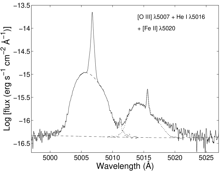
Figure 4: The intermediate and narrow components of [O III] $\lambda$5006.8 and He I $\lambda$5016 for the northern part of the ER. The dashed lines show the estimated zero intensity levels for the narrow and intermediate components, respectively. The red wing of the intermediate component of [O III] is blended with He I $\lambda$ 5015.7. He I $\lambda$ 5875.6 is used as a template for He I $\lambda$ 5015.7 and the dotted line shows the result of the deblending procedure. Note also [Fe II] $\lambda$5020.2 that gives the excess flux in the red wing of He I $\lambda$ 5015.7. The wavelength scale is corrected for redshift.

The line profile of the narrow components is mainly due to thermal broadening at least for the lightest elements such as H and He. However, since the ER is an extended object, the observed profile will deviate from a simple Gaussian, looking more like a skewed Gaussian (see Fig. 5). By contrast, the line profile of the intermediate component is dominated by shock dynamics and there is no reason for it to be Gaussian at all. Figure 4 shows [O III] $\lambda$5007 and He I $5016$ for the two components. In Sect. 4 we will discuss the physical cause of the line profiles in more detail.

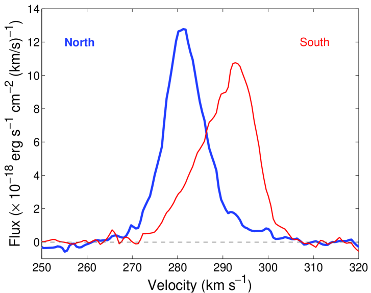
Figure 5: [Fe II] $\lambda$7155 line profiles from the northern (thick line) and southern (thin line) parts of the ER. The velocity scale is heliocentric. The lines appear as skewed Gaussians due to contributions from the opposite side of the ring in both cases. See text for more details.

Identifications of all emission lines are given in Table LABEL:tab:ions, and measurements of the velocities and fluxes of the most significant emission lines are presented in Tables LABEL:tab:narrowlines–LABEL:tab:broadlinesS. The values listed in the tables were obtained by fitting a sum of Gaussians to the line profiles and the background was estimated by a third-order polynomial interpolation. The values given in brackets are the statistical $1\sigma$ uncertainties of these fits. We note, however, that the systematic errors in the relative fluxes are $10-15$%, which in many cases dominate over the statistical errors.

The velocity ranges of the intermediate components ($V_{\rm blue}$ and $V_{\rm red}$) are defined as the ranges where the flux is more than $5\%$ of the peak flux. The reason for using this, rather than the maximum extent of the line, is that the latter is very sensitive to the signal-to-noise ratio (S/N) of the line, which varies by a factor of $\ga 100$. With this measure we can therefore better compare lines of very different fluxes. The maximum extent is discussed in Sect. 4.2.3.

The peak velocities for the narrow components are with respect to the heliocentric motion, whereas the peak velocities for the intermediate components are relative to the peak velocity of the corresponding narrow component. This provides a natural frame for the ejecta impact on the ER. For the extinction we adopted a reddening of $E(B-V)=0.16{\rm\leavevmode\nobreak\ mag}$ (Fitzpatrick & Walborn 1990) with $E(B-V)=0.06{\rm\leavevmode\nobreak\ mag}$ from the Milky way (e.g., Staveley-Smith et al. 2003) and $E(B-V)=0.10{\rm\leavevmode\nobreak\ mag}$ from the LMC. The reddening law was taken from Cardelli et al. (1989) using $R_{V}=3.1$.

Table 2: The dereddened Balmer line fluxes relative to H$\beta$ for the unshocked gas. Only the 1$\sigma$ statistical errors are given. Systematic errors are discussed in the text.

Position	H$\alpha$	H$\beta$	H$\gamma$	H$\delta$
north	$354.2\pm 1.1$	$100$	$47.0\pm 0.3$	$22.5\pm 0.2$
south	$322.8\pm 1.0$	$100$	$43.5\pm 0.3$	$17.9\pm 0.1$
Case B	$287$	$100$	$46.6$	$25.6$

Table 3: Emission lines grouped by ions.

Ion	Wavelengths ( Å)
H I	3691.6b, 3697.2, 3703.9, 3712.0, 3721.9, 3734.4, 3750.2, 3770.6, 3797.9, 3835.4, 3889.0, 3970.1, 4101.7, 4340.5,
	4861.3, 6562.8, 8438.0, 8467.3, 8502.5, 8665.0, 8750.5, 8862.8, 9014.9, 9229.0, 9546.0, 10049.4
He I	3187.7, 3705.0, 3819.6, 3888.7, 4026.2, 4120.8b, 4143.8, 4387.9, 4471.5, 4713.2, 4921.9, 5015.7, 5047.7, 5875.7,
	6678.2, 6855.9b, 7065.7, 7281.4, 8444.5a, 8530.9a, 8662.2a
He II	3203.1b, 3710.4a, 4541.6b, 4685.7, 5411.5, 5431.8b, 6527.1a, 8236.8a
C I	8727.1b
N I	3466.5b, 5197.9, 5200.3
N II	5754.5, 6547.9, 6583.3
O I	5577.3, 6300.3, 6363.8, 7254.2-5a, 8446.3-8a
O II	3726.0a, 3728.8a, 7318.9, 7320.0, 7329.7,7330.7
O III	4363.2, 4958.9, 5006.8
Ne III	3868.8, 3967.5
Ne IV	4714.2, 4725.7b
Ne V	3345.9a, 3425.9
Mg I	4562.7a, 4571.1
Si II	5041.0a, 5056.0a, 6347.1a, 6371.4a
S II	4068.6, 4076.4, 6716.4, 6730.8
S III	6312.1, 9068.6, 9530.6
Cl II	9123.6a
Ar III	7135.8, 7751.1
Ar IV	4711.3a, 4740.1a
Ar V	7005.7a
Ca II	3933.7, 7291.5, 7323.9
Ca V	5309.1a, 6086.4a
Cr II	4580.8, 4581.1, 8000.1, 8125.3, 8229.7, 8308.5, 8357.6
Fe II	4114.5b, 4177.2b, 4244.0, 4276.8, 4287.4, 4305.9b, 4319.6b, 4346.9b, 4352.8b, 4358.4b, 4359.3a, 4372.4b, 4416.3,
	4452.1b, 4457.9b, 4639.7b, 4774.7b, 4798.3b, 4814.5, 4874.5b, 4889.6, 4905.3, 4950.7b, 4973.4b, 5072.4b, 5111.6,
	5158.8, 5220.1, 5261.6, 5268.9b, 5273.3, 5296.8b, 5333.6, 5376.5, 5433.1b, 5477.2b, 5494.3b, 5527.6, 5721.3, 5745.7,
	6440.4b, 6872.2b, 6896.2b, 6944.9b, 7155.2, 7172.0, 7388.2, 7452.5, 7637.5, 7686.9, 8891.9, 9051.9, 9226.6, 9267.6
Fe III	4658.1, 4701.5, 4754.7, 4769.4b, 4881.0a, 5011.3a, 5270.4a
Fe V	4227.2a
Fe VI	4972.5a, 5277.8, 5335.2a
Fe VII	3586.3b, 4893.4a, 5720.7, 6087.0
Fe X	6374.5b
Fe XI	7891.8b
Fe XIV	5302.9b
Ni II	6666.8b, 7377.8, 7411.6b

• Only a narrow component is detected.

• Only an intermediate component is detected.

Table 4: Emission lines from the unshocked gas of the ER.

			North			South		Extinction
Emission	Rest wavel.	Relative fluxa	$V_{\rm peak}^{\mathrm{b}}$	$V_{\rm fwhm}$	Relative fluxa	$V_{\rm peak}^{\mathrm{b}}$	$V_{\rm fwhm}$	correctionc
	$(\mbox{ \AA})$		($\rm\leavevmode\nobreak\ km\leavevmode\nobreak\ s^{-1}$)	$(\rm\leavevmode\nobreak\ km\leavevmode\nobreak\ s^{-1}$)		($\rm\leavevmode\nobreak\ km\leavevmode\nobreak\ s^{-1}$)	$(\rm\leavevmode\nobreak\ km\leavevmode\nobreak\ s^{-1})$
[Ne V]	3425.86	$\phantom{00}17.2\pm\phantom{0}1.7$	$281.7\pm 1.2$	$23.45\pm 0.58$	$\phantom{00}13.8\pm\phantom{0}1.6$	$294.4\pm 1.0$	$19.55\pm 0.57$	2.06
[O II]	3726.03	$\phantom{0}109.2\pm\phantom{0}4.1$	$283.0\pm 0.4$	$13.82\pm 0.13$	$\phantom{0}101.1\pm\phantom{0}4.0$	$293.3\pm 0.5$	$14.77\pm 0.23$	1.98
[O II]	3728.82	$\phantom{00}66.4\pm\phantom{0}3.7$	$280.1\pm 0.5$	$14.19\pm 0.20$	$\phantom{00}63.8\pm\phantom{0}3.9$	$290.6\pm 0.6$	$14.87\pm 0.37$	1.98
[Ne III]	3868.75	$\phantom{00}44.0\pm\phantom{0}1.8$	$281.3\pm 0.5$	$15.72\pm 0.18$	$\phantom{00}24.7\pm\phantom{0}1.8$	$292.1\pm 0.7$	$17.64\pm 0.28$	1.94
[S II]	4068.60	$\phantom{00}17.0\pm\phantom{0}0.9$	$281.3\pm 0.4$	$11.07\pm 0.15$	$\phantom{00}15.2\pm\phantom{0}0.8$	$291.3\pm 0.6$	$13.77\pm 0.22$	1.90
[S II]	4076.35	$\phantom{000}5.4\pm\phantom{0}0.6$	$281.7\pm 0.6$	$11.46\pm 0.30$	$\phantom{000}5.1\pm\phantom{0}0.6$	$292.2\pm 0.9$	$13.60\pm 0.44$	1.90
H$\delta$	4101.73	$\phantom{00}20.3\pm\phantom{0}0.8$	$281.7\pm 1.0$	$28.43\pm 0.36$	$\phantom{00}15.6\pm\phantom{0}0.6$	$290.9\pm 0.8$	$24.72\pm 0.29$	1.89
H$\gamma$	4340.46	$\phantom{00}44.6\pm\phantom{0}1.7$	$281.1\pm 1.0$	$25.86\pm 0.26$	$\phantom{00}39.4\pm\phantom{0}1.6$	$291.0\pm 0.8$	$26.52\pm 0.24$	1.84
[O III]	4363.21	$\phantom{00}10.6\pm\phantom{0}0.7$	$279.3\pm 0.7$	$17.55\pm 0.31$	$\phantom{000}6.7\pm\phantom{0}0.6$	$290.8\pm 1.0$	$23.97\pm 0.64$	1.84
He II	4685.70	$\phantom{00}10.1\pm\phantom{0}1.4$	$283.0\pm 1.2$	$21.56\pm 1.27$	$\phantom{000}7.1\pm\phantom{0}0.7$	$295.6\pm 1.6$	$30.39\pm 1.41$	1.75
H$\beta$	4861.32	$\phantom{0}100.0$	$280.9\pm 0.5$	$26.04\pm 0.11$	$\phantom{00}97.9\pm\phantom{0}2.6$	$290.6\pm 0.6$	$27.36\pm 0.16$	1.71
[O III]	4958.91	$\phantom{00}81.3\pm\phantom{0}2.1$	$281.0\pm 0.4$	$15.69\pm 0.11$	$\phantom{00}50.1\pm\phantom{0}1.3$	$291.8\pm 0.5$	$22.38\pm 0.14$	1.68
[O III]	5006.84	$\phantom{0}247.2\pm\phantom{0}5.1$	$281.1\pm 0.3$	$15.88\pm 0.06$	$\phantom{0}154.9\pm\phantom{0}3.5$	$292.5\pm 0.5$	$22.85\pm 0.10$	1.67
[O I]	5577.34	$\phantom{000}0.5\pm\phantom{0}0.2$	$283.4\pm 1.4$	$14.66\pm 1.17$	$\phantom{000}0.5\pm\phantom{0}0.2$	$289.5\pm 1.4$	$15.19\pm 1.23$	1.57
[N II]	5754.59	$\phantom{00}20.6\pm\phantom{0}0.6$	$281.5\pm 0.3$	$13.69\pm 0.09$	$\phantom{00}19.3\pm\phantom{0}0.5$	$292.0\pm 0.4$	$16.21\pm 0.16$	1.54
He I	5875.63	$\phantom{00}17.3\pm\phantom{0}0.6$	$280.8\pm 0.5$	$16.85\pm 0.15$	$\phantom{00}16.9\pm\phantom{0}0.6$	$290.3\pm 0.5$	$18.63\pm 0.16$	1.53
[O I]	6300.30	$\phantom{00}48.0\pm\phantom{0}1.9$	$281.4\pm 0.4$	$11.67\pm 0.12$	$\phantom{00}47.7\pm\phantom{0}1.4$	$291.2\pm 0.4$	$14.12\pm 0.16$	1.47
[S III]	6312.06	$\phantom{000}2.6\pm\phantom{0}0.3$	$280.6\pm 0.7$	$12.78\pm 0.47$	$\phantom{000}1.3\pm\phantom{0}0.2$	$291.9\pm 1.3$	$18.49\pm 0.85$	1.47
[O I]	6363.78	$\phantom{00}16.1\pm\phantom{0}0.6$	$281.1\pm 0.3$	$11.40\pm 0.09$	$\phantom{00}16.7\pm\phantom{0}0.4$	$291.6\pm 0.4$	$14.50\pm 0.12$	1.47
[N II]	6548.05	$\phantom{0}359.9\pm\phantom{0}7.3$	$281.9\pm 0.3$	$12.95\pm 0.05$	$\phantom{0}352.7\pm\phantom{0}6.9$	$292.5\pm 0.3$	$14.88\pm 0.05$	1.45
H$\alpha$	6562.80	$\phantom{0}419.2\pm\phantom{0}6.9$	$280.9\pm 0.4$	$28.69\pm 0.07$	$\phantom{0}369.8\pm\phantom{0}5.7$	$290.5\pm 0.3$	$27.82\pm 0.05$	1.45
[N II]	6583.45	$1112.7\pm 18.7$	$280.7\pm 0.2$	$12.74\pm 0.03$	$1096.4\pm 18.2$	$291.2\pm 0.2$	$14.99\pm 0.04$	1.45
He I	6678.15	$\phantom{000}5.5\pm\phantom{0}0.6$	$281.1\pm 0.7$	$16.07\pm 0.35$	$\phantom{000}4.7\pm\phantom{0}0.3$	$291.6\pm 0.7$	$18.12\pm 0.32$	1.44
[S II]	6716.44	$\phantom{00}62.2\pm\phantom{0}1.5$	$281.9\pm 0.3$	$11.61\pm 0.06$	$\phantom{00}69.6\pm\phantom{0}1.8$	$292.9\pm 0.3$	$13.75\pm 0.07$	1.43
[S II]	6730.82	$\phantom{0}103.5\pm\phantom{0}2.4$	$281.7\pm 0.3$	$11.46\pm 0.06$	$\phantom{0}115.5\pm\phantom{0}3.3$	$292.7\pm 0.3$	$13.82\pm 0.08$	1.43
[Ar III]	7135.79	$\phantom{000}8.3\pm\phantom{0}0.4$	$279.9\pm 0.4$	$12.91\pm 0.15$	$\phantom{000}5.4\pm\phantom{0}0.4$	$290.1\pm 0.7$	$18.11\pm 0.29$	1.39
[Fe II]	7155.16	$\phantom{000}4.8\pm\phantom{0}0.3$	$281.3\pm 0.4$	$\phantom{0}9.91\pm 0.13$	$\phantom{000}4.9\pm\phantom{0}0.2$	$293.2\pm 0.4$	$13.73\pm 0.28$	1.39
[O II]	7319d00	$\phantom{00}13.1\pm\phantom{0}1.0$	-	-	$\phantom{00}12.3\pm\phantom{0}0.7$	-	-	1.37
[Ca II]	7323.89	$\phantom{000}7.2\pm\phantom{0}0.3$	$279.9\pm 0.4$	$\phantom{0}9.77\pm 0.13$	$\phantom{000}9.8\pm\phantom{0}0.3$	$291.9\pm 0.4$	$13.39\pm 0.21$	1.37
[O II]	7330${}^{\mathrm{e}}\phantom{00}$	$\phantom{00}11.4\pm\phantom{0}0.8$	-	-	$\phantom{000}9.5\pm\phantom{0}0.8$	-	-	1.37
[S III]	9068.60	$\phantom{00}21.5\pm\phantom{0}0.7$	-	$12.76\pm 0.10$	$\phantom{00}11.2\pm\phantom{0}0.4$	-	$18.90\pm 0.17$	1.24
[S III]	9531.10	$\phantom{00}55.2\pm\phantom{0}2.0$	-	$12.84\pm 0.12$	$\phantom{00}27.8\pm\phantom{0}0.9$	-	$17.58\pm 0.22$	1.22

• Fluxes are relative to the flux of H$\beta$ in the Northern ER: “100” corresponds to $(31.3\pm 0.5)\times 10^{-16}\rm\leavevmode\nobreak\ erg\leavevmode\nobreak\ s^{-1}cm^{-2}$. Fluxes are not corrected for the extinction. The errors are only statistical, and do not include systematic uncertaities (see text).

• The recession velocity of the peak flux.

• $E(B-V)=0.16{\rm\leavevmode\nobreak\ mag}$, with $E(B-V)=0.10{\rm\leavevmode\nobreak\ mag}$ for LMC and $E(B-V)=0.06{\rm\leavevmode\nobreak\ mag}$ for the Milky Way.

• Applies to both lines at 7318.92 Å and 7319.99 Å.

• Applies to both lines at 7329.67 Å and 7330.73 Å.

Table 5: Emission lines from the shocked gas of the northern ER.

Emission	Rest wavel.	Relative fluxa	$V_{\rm peak}^{\mathrm{b}}$	$V_{\rm blue}^{\mathrm{c}}$	$V_{\rm red}^{\mathrm{c}}$	Extinction
	$(\mbox{ \AA})$		($\rm\leavevmode\nobreak\ km\leavevmode\nobreak\ s^{-1}$)	($\rm\leavevmode\nobreak\ km\leavevmode\nobreak\ s^{-1}$)	($\rm\leavevmode\nobreak\ km\leavevmode\nobreak\ s^{-1}$)	correctiond
[Ne V]	3425.86	$\phantom{00}14.8\pm\phantom{0}3.6$	$-136.3\pm 21.4$	$-259.1\pm 34.9$	$202.9\pm 43.3$	2.06
[Ne III]	3868.75	$\phantom{0}111.1\pm\phantom{0}3.6$	$-\phantom{0}87.8\pm\phantom{0}6.2$	$-263.1\pm\phantom{0}4.0$	$216.9\pm\phantom{0}8.9$	1.94
[S II]	4068.60	$\phantom{0}171.5\pm\phantom{0}4.6$	$-\phantom{0}77.2\pm\phantom{0}4.3$	$-240.5\pm\phantom{0}4.7$	$180.4\pm\phantom{0}5.5$	1.90
[S II]	4076.35	$\phantom{00}45.7\pm\phantom{0}2.1$	$-\phantom{0}76.9\pm\phantom{0}6.3$	$-254.9\pm\phantom{0}5.3$	$203.0\pm 11.2$	1.90
H$\delta$	4101.73	$\phantom{0}105.5\pm\phantom{0}2.6$	$-\phantom{0}86.8\pm\phantom{0}4.7$	$-261.4\pm\phantom{0}2.4$	$197.5\pm\phantom{0}6.6$	1.89
H$\gamma$	4340.46	$\phantom{0}223.4\pm\phantom{0}5.0$	$-\phantom{0}88.4\pm\phantom{0}4.2$	$-260.0\pm\phantom{0}2.5$	$180.5\pm\phantom{0}4.1$	1.84
[O III]	4363.21	$\phantom{00}32.0\pm\phantom{0}2.0$	$-\phantom{0}67.5\pm\phantom{0}7.0$	$-251.5\pm\phantom{0}8.0$	$187.7\pm 15.1$	1.84
[Fe III]	4658.05	$\phantom{000}9.8\pm\phantom{0}1.1$	$-101.2\pm 11.5$	$-270.9\pm 17.3$	$204.9\pm 37.8$	1.76
He II	4685.70	$\phantom{00}37.3\pm\phantom{0}1.7$	$-\phantom{0}94.7\pm\phantom{0}6.8$	$-265.9\pm\phantom{0}5.8$	$182.8\pm 13.1$	1.75
H$\beta$	4861.32	$\phantom{0}524.4\pm\phantom{0}8.2$	$-\phantom{0}85.9\pm\phantom{0}3.2$	$-258.7\pm\phantom{0}1.1$	$189.1\pm\phantom{0}1.8$	1.71
[O III]	4958.91	$\phantom{00}45.7\pm\phantom{0}1.7$	$-\phantom{0}66.1\pm\phantom{0}7.3$	$-243.7\pm\phantom{0}5.6$	$179.4\pm\phantom{0}6.9$	1.68
[O III]	5006.84	$\phantom{0}140.0\pm\phantom{0}2.7$	$-\phantom{0}58.5\pm\phantom{0}4.4$	$-252.5\pm\phantom{0}2.9$	$212.8\pm\phantom{0}3.3$	1.67
[Fe XIV]	5302.86	$\phantom{00}12.2\pm\phantom{0}1.0$	$-132.8\pm 11.5$	$-386.7\pm 10.7$	$352.3\pm 46.7$	1.61
[O I]	5577.34	$\phantom{00}16.6\pm\phantom{0}1.0$	$-\phantom{0}90.3\pm\phantom{0}7.0$	$-253.7\pm\phantom{0}5.2$	$194.4\pm 16.9$	1.57
[N II]	5754.59	$\phantom{0}223.7\pm\phantom{0}3.7$	$-\phantom{0}89.6\pm\phantom{0}3.4$	$-252.7\pm\phantom{0}1.3$	$187.3\pm\phantom{0}2.0$	1.54
He I	5875.63	$\phantom{0}156.1\pm\phantom{0}2.6$	$-\phantom{0}84.3\pm\phantom{0}3.5$	$-253.3\pm\phantom{0}1.4$	$191.5\pm\phantom{0}2.3$	1.53
[Fe VII]	6087.00	$\phantom{000}2.3\pm\phantom{0}0.4$	$-102.6\pm 16.4$	$-345.6\pm 22.4$	$139.9\pm 22.2$	1.50
[O I]	6300.30	$\phantom{0}237.4\pm\phantom{0}3.7$	$-\phantom{0}76.9\pm\phantom{0}2.0$	$-229.9\pm\phantom{0}0.8$	$169.0\pm\phantom{0}1.8$	1.47
[S III]	6312.06	$\phantom{00}11.4\pm\phantom{0}0.8$	$-\phantom{0}92.8\pm\phantom{0}9.3$	$-254.1\pm\phantom{0}9.1$	$185.2\pm 18.9$	1.47
[O I]	6363.78	$\phantom{00}81.3\pm\phantom{0}2.6$	$-\phantom{0}76.6\pm\phantom{0}4.2$	$-233.0\pm\phantom{0}5.2$	$184.0\pm\phantom{0}7.2$	1.47
[Fe X]	6374.51	$\phantom{000}9.8\pm\phantom{0}0.8$	$-127.8\pm 10.9$	$-348.7\pm 11.7$	$156.2\pm 20.7$	1.47
[N II]	6548.05	$\phantom{00}75.6\pm\phantom{0}1.7$	$-\phantom{0}80.8\pm\phantom{0}4.5$	$-247.4\pm\phantom{0}2.7$	$178.6\pm\phantom{0}3.5$	1.45
H$\alpha$	6562.80	$2112.2\pm 31.0$	$-\phantom{0}82.1\pm\phantom{0}2.7$	$-259.8\pm\phantom{0}0.9$	$195.4\pm\phantom{0}0.9$	1.45
[N II]	6583.45	$\phantom{0}227.5\pm\phantom{0}3.7$	$-\phantom{0}78.2\pm\phantom{0}3.2$	$-244.0\pm\phantom{0}1.5$	$183.0\pm\phantom{0}1.6$	1.45
He I	6678.15	$\phantom{00}38.2\pm\phantom{0}1.2$	$-\phantom{0}89.6\pm\phantom{0}4.9$	$-261.9\pm\phantom{0}3.5$	$194.6\pm\phantom{0}8.0$	1.44
[S II]	6716.44	$\phantom{000}4.6\pm\phantom{0}0.3$	$-\phantom{0}45.2\pm\phantom{0}8.4$	$-232.2\pm\phantom{0}7.2$	$144.8\pm\phantom{0}7.1$	1.43
[S II]	6730.82	$\phantom{000}9.9\pm\phantom{0}0.8$	$-\phantom{0}61.5\pm\phantom{0}7.7$	$-239.2\pm 19.6$	$214.0\pm 29.0$	1.43
[Ar V]	7005.67	$\phantom{000}1.2\pm\phantom{0}0.3$	$-\phantom{0}89.5\pm 22.3$	$-347.6\pm 35.3$	$183.7\pm 34.3$	1.41
[Ar III]	7135.79	$\phantom{00}18.9\pm\phantom{0}0.9$	$-\phantom{0}73.8\pm 10.4$	$-255.8\pm\phantom{0}5.7$	$187.9\pm 10.6$	1.39
[Fe II]	7155.16	$\phantom{00}43.3\pm\phantom{0}0.9$	$-\phantom{0}85.9\pm\phantom{0}2.9$	$-245.3\pm\phantom{0}3.0$	$170.2\pm\phantom{0}4.2$	1.39
[Fe XI]	7891.94	$\phantom{000}9.7\pm\phantom{0}0.9$	$-125.9\pm\phantom{0}9.8$	$-336.1\pm 27.0$	$218.1\pm 25.1$	1.32
[S III]	9068.60	$\phantom{00}15.8\pm\phantom{0}0.9$	$-\phantom{0}53.4\pm\phantom{0}8.3$	$-241.0\pm 12.3$	$138.6\pm\phantom{0}6.6$	1.24
[S III]	9531.10	$\phantom{00}57.4\pm\phantom{0}1.7$	$-\phantom{0}81.6\pm\phantom{0}6.9$	$-267.2\pm\phantom{0}4.5$	$172.3\pm\phantom{0}6.1$	1.22

• Fluxes are relative to the flux of H$\beta$ of the unshocked component in the Northern ER: “100” corresponds to $(31.3\pm 0.5)\times 10^{-16}\rm\leavevmode\nobreak\ erg\leavevmode\nobreak\ s^{-1}cm^{-2}$. Fluxes are not corrected for the extinction. The errors are only statistical, and do not include systematic uncertaities (see text).

• The velocities are relative to the unshocked, narrow component of the emission lines.

• The velocity where fluxes are $5\%$ of the peak flux.

• $E(B-V)=0.16{\rm\leavevmode\nobreak\ mag}$, with $E(B-V)=0.10{\rm\leavevmode\nobreak\ mag}$ for LMC and $E(B-V)=0.06{\rm\leavevmode\nobreak\ mag}$ for the Milky Way.

Table 6: Emission lines from the shocked gas of the southern ER.

Emission	Rest wavel.	Relative fluxa	$V_{\rm peak}^{\mathrm{b}}$	$V_{\rm blue}^{\mathrm{c}}$	$V_{\rm red}^{\mathrm{c}}$	Extinction
	$(\mbox{ \AA}$)		($\rm\leavevmode\nobreak\ km\leavevmode\nobreak\ s^{-1}$)	($\rm\leavevmode\nobreak\ km\leavevmode\nobreak\ s^{-1}$)	($\rm\leavevmode\nobreak\ km\leavevmode\nobreak\ s^{-1}$)	correctiond
[Ne V]	3425.86	$\phantom{00}6.0\pm 1.7$	$\phantom{0}9.8\pm 28.6$	$-247.6\pm 47.2$	$260.7\pm 46.1$	2.06
[Ne III]	3868.75	$\phantom{0}29.5\pm 1.5$	$31.7\pm\phantom{0}8.2$	$-173.2\pm\phantom{0}6.7$	$236.4\pm\phantom{0}6.7$	1.94
[S II]	4068.60	$\phantom{0}41.2\pm 2.1$	$31.7\pm\phantom{0}8.2$	$-114.5\pm\phantom{0}6.6$	$192.6\pm\phantom{0}8.1$	1.90
[S II]	4076.35	$\phantom{0}12.6\pm 0.9$	$32.8\pm\phantom{0}9.4$	$-168.2\pm\phantom{0}9.0$	$237.2\pm\phantom{0}9.0$	1.90
H$\delta$	4101.73	$\phantom{0}26.5\pm 1.9$	$18.8\pm\phantom{0}8.0$	$-118.6\pm\phantom{0}9.1$	$215.2\pm 12.1$	1.89
H$\gamma$	4340.46	$\phantom{0}57.4\pm 2.0$	$28.7\pm\phantom{0}7.2$	$-147.5\pm\phantom{0}5.5$	$210.5\pm\phantom{0}5.9$	1.84
[O III]	4363.21	$\phantom{0}10.4\pm 1.3$	$32.9\pm\phantom{0}8.6$	$-168.9\pm\phantom{0}7.8$	$222.7\pm\phantom{0}7.8$	1.84
[Fe III]	4658.05	$\phantom{00}3.1\pm 0.6$	$12.8\pm 18.7$	$-232.3\pm 28.6$	$259.6\pm 28.1$	1.76
He II	4685.70	$\phantom{0}10.1\pm 1.2$	$39.5\pm 15.6$	$-170.9\pm 20.0$	$224.2\pm 20.0$	1.75
H$\beta$	4861.32	$149.8\pm 2.9$	$34.1\pm\phantom{0}3.7$	$-175.1\pm\phantom{0}3.5$	$218.5\pm\phantom{0}2.0$	1.71
[O III]	4958.91	$\phantom{0}18.3\pm 0.8$	$14.3\pm\phantom{0}6.2$	$-226.3\pm 12.9$	$204.0\pm\phantom{0}6.0$	1.68
[O III]	5006.84	$\phantom{0}55.3\pm 1.5$	$16.4\pm\phantom{0}7.0$	$-214.4\pm\phantom{0}5.8$	$215.6\pm\phantom{0}5.0$	1.67
[O I]	5577.34	$\phantom{00}3.5\pm 0.4$	$38.5\pm\phantom{0}9.3$	$-141.2\pm 10.0$	$214.8\pm 10.0$	1.57
[N II]	5754.59	$\phantom{0}63.5\pm 1.4$	$40.7\pm\phantom{0}5.9$	$-188.0\pm\phantom{0}3.6$	$207.9\pm\phantom{0}3.0$	1.54
He I	5875.63	$\phantom{0}49.7\pm 1.2$	$38.2\pm\phantom{0}5.4$	$-215.0\pm\phantom{0}3.0$	$231.6\pm\phantom{0}4.9$	1.53
[O I]	6300.30	$\phantom{0}69.1\pm 1.3$	$32.5\pm\phantom{0}5.1$	$-162.4\pm\phantom{0}1.8$	$193.7\pm\phantom{0}3.8$	1.47
[S III]	6312.06	$\phantom{00}2.6\pm 0.4$	$24.7\pm 12.5$	$-158.5\pm 16.8$	$213.0\pm 16.8$	1.47
[O I]	6363.78	$\phantom{0}21.7\pm 0.8$	$27.1\pm\phantom{0}9.2$	$-143.7\pm\phantom{0}5.4$	$175.1\pm\phantom{0}3.7$	1.47
[N II]	6548.05	$\phantom{0}24.3\pm 0.8$	$31.5\pm\phantom{0}6.0$	$-190.8\pm\phantom{0}4.1$	$196.6\pm\phantom{0}6.6$	1.45
H$\alpha$	6562.80	$582.0\pm 8.7$	$36.0\pm\phantom{0}2.5$	$-190.9\pm\phantom{0}1.2$	$223.2\pm\phantom{0}0.9$	1.45
[N II]	6583.45	$\phantom{0}76.1\pm 1.4$	$28.8\pm\phantom{0}3.6$	$-184.2\pm\phantom{0}2.9$	$194.2\pm\phantom{0}1.6$	1.45
He I	6678.15	$\phantom{0}10.0\pm 0.5$	$31.4\pm\phantom{0}8.1$	$-188.4\pm\phantom{0}6.3$	$252.8\pm\phantom{0}6.3$	1.44
[S II]	6716.44	$\phantom{00}1.3\pm 0.2$	$20.1\pm 10.0$	$-124.3\pm 13.7$	$167.1\pm 13.7$	1.43
[S II]	6730.82	$\phantom{00}3.1\pm 0.4$	$27.5\pm 10.3$	$-146.0\pm 12.4$	$202.4\pm 12.4$	1.43
[Ar III]	7135.79	$\phantom{00}5.9\pm 0.6$	$19.6\pm 14.5$	$-196.2\pm 20.1$	$217.6\pm 15.7$	1.39
[Fe II]	7155.16	$\phantom{0}11.2\pm 0.5$	$14.1\pm\phantom{0}6.3$	$-184.2\pm\phantom{0}9.1$	$199.8\pm\phantom{0}8.4$	1.39
[S III]	9068.60	$\phantom{00}6.8\pm 0.8$	$-0.1\pm 17.5$	$-272.7\pm 24.0$	$240.4\pm 42.0$	1.24
[S III]	9531.10	$\phantom{0}16.5\pm 1.4$	$23.4\pm\phantom{0}8.5$	$-275.5\pm 25.7$	$216.7\pm 12.5$	1.22

• Fluxes are relative to the flux of H$\beta$ of the unshocked component in the Northern ER: “100” corresponds to $(31.3\pm 0.5)\times 10^{-16}\rm\leavevmode\nobreak\ erg\leavevmode\nobreak\ s^{-1}cm^{-2}$. Fluxes are not corrected for the extinction. The errors are only statistical, and do not include systematic uncertaities (see text).

• The velocities are relative to the unshocked, narrow component of the emission lines.

• The velocity where fluxes are $5\%$ of the peak flux.

• $E(B-V)=0.16{\rm\leavevmode\nobreak\ mag}$, with $E(B-V)=0.10{\rm\leavevmode\nobreak\ mag}$ for LMC and $E(B-V)=0.06{\rm\leavevmode\nobreak\ mag}$ for the Milky Way.

4 Analysis

4.1 The narrow component

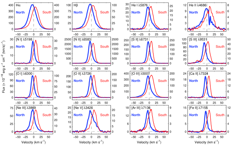
Figure 6: Line profiles of the narrow emission lines from the northern (blue/thick lines) and southern (red/thin lines) parts of the ER. The zero velocity corresponds to the rest frame of the SN ($286.5\rm\leavevmode\nobreak\ km\leavevmode\nobreak\ s^{-1}$). The left y-axis indicate the flux of the emission lines from the northern part of the ER and the right y-axis indicate the flux from the southern part. The line profiles have been smoothed using a fourth-order Savitzky-Golay filter. Note the thermal broadening of the lighter elements.

The dereddened Balmer lines ratios (relative to H$\beta$) are listed in Table LABEL:tab:balmerflux, together with the theoretical values given for case B at $10^{4}$ K and a gas density of $10^{4}{\rm\leavevmode\nobreak\ cm^{-3}}$ (Osterbrock 1989). In general, the ratios we find are close to those predicted by Case B theory, except for our high $j_{{\rm H}\alpha}/j_{{\rm H}\beta}$ ratios. For both the unshocked and shocked (cf. Sect. 4.2.1) gas, the H$\beta$ flux appears to be stronger relative to the other Balmer lines on the southern side of the ring than the northern, maybe by $\sim 10\%$. Given the systematic uncertainty in the relative fluxes, this difference is hardly significant. We note, however, that collisional excitation of H$\alpha$ may be important for the narrow lines (see Lundqvist & Fransson 1996).

To estimate the temperature and density of the unshocked ER, we have adopted a nebular analysis. For O II, S II and S III we have used a five-level atom, and for N II, O I and O III a six-level atom. Atomic data for N II, O III, and S II are the same as described in Maran et al. (2000), and for O II we included data from Osterbrock (1989) and McLaughlin & Bell (1993). Data for S III are from Hayes (1986), Galavis et al. (1995) and Tayal (1997).

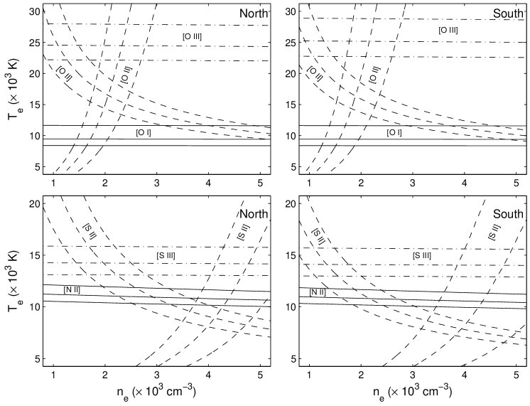
Figure 7: Electron density vs. temperature for the dereddened line ratios of emission from the unshocked gas. The left panels show the emission from the northern part of the ring and the right panels are for the southern part. The line ratios are: [O I] $\lambda\lambda 6300,6364/\lambda 5577$, [O II] ($\lambda\lambda 7319-7331/\lambda\lambda 3726,3729$ and $\lambda 3729/\lambda 3726$), [O III] $\lambda\lambda 4959,5007/\lambda 4363$, [N II] $\lambda\lambda 6548,6583/\lambda 5755$, [S II] ($\lambda\lambda 4069,4076/\lambda\lambda 6716,6731$ and $\lambda 6716/\lambda 6731$), [S III] ($\lambda\lambda 9069,9531/\lambda 6312$). Each solution curve is embraced by error curves of at least 15% to account for the systematic relative flux uncertainties. The exception is for $\lambda 3729/\lambda 3726$ and $\lambda 6716/\lambda 6731$ ratios for which the systematic errors should be small. Instead these are embraced by the $1\sigma$ statistical error curves. Note how the rather temperature insensitive ratios $\lambda 3729/\lambda 3726$ and $\lambda 6716/\lambda 6731$ together with the temperature sensitive ratios $\lambda\lambda 7319-7331/\lambda\lambda 3726,3729$ and $\lambda\lambda 4069,4076/\lambda\lambda 6716,6731$ can constrain both the density and temperature of [O II] and [S II].

In Fig. 7 we show the allowed temperature-density range for both parts of the ER, using our six-level atoms for [N II] and [O III]. As discussed by Maran et al. (2000), the narrow emission lines at these late epochs are expected to mainly come from gas with density significantly below $10^{4}\mbox{ cm}^{-3}$. Below this density our [O III] temperatures should be in the range $(2.5\pm 0.3)\times 10^{4}$ K, and the [N II] temperatures should be confined to the range $(1.1\pm 0.1)\times 10^{4}$ K, where the errors stated include statistical errors as well as a $\pm 10$% systematic error (see Sect. 2.1). These results are in general in very good agreement with the estimates of Maran et al. (2000), who obtained [N II] temperatures in the range $9.5\times 10^{3}-1.3\times 10^{4}$ K and [O III] temperatures in excess of $\sim 1.7\times 10^{4}$ K, using HST/STIS data from 1998 November 14, with perhaps a slightly higher [N II] temperature in the western ER ($\mathrm{PA}=283^{\circ}$) than in the eastern ($\mathrm{PA}=103^{\circ}$). We find no clear evidence for a temperature difference between the northern and southern parts of the ER.

To get a further handle on the temperature, we can use [O II] $\lambda\lambda$3726, 3729 in combination with [O II] $\lambda\lambda$7319-7330, as well as [S II] $\lambda\lambda$4069, 4076 in combination with [S II] $\lambda\lambda$6716, 6731. The results from our five-level model atoms are plotted in Fig. 7. As the $j_{\lambda 3729}/j_{\lambda 3726}$ and $j_{\lambda 6716}/j_{\lambda 6731}$ intensity ratios are rather insensitive to temperature, but the other ratios, i.e., $j_{\lambda\lambda 7319-7331}/j_{\lambda\lambda 3726,3729}$ and $j_{\lambda\lambda 4069,4076}/j_{\lambda\lambda 6716,6731}$ are temperature sensitive, these figures can be used to determine temperature and density simultaneously for [O II] and [S II]. This has not been done previously for the ER and provides a more accurate determination as input for models such as those of Lundqvist & Fransson (1996). For [O II] there is an overlap in temperature ($(1.7\pm 0.5)\times 10^{4}$ K) as well as in electron density, $(2.0\pm 0.5)\times 10^{3}\mbox{ cm}^{-3}$, of the two parts of the ER. For [S II], the overall preferred range of electron density vs. temperature is in this case $(4\pm 1)\times 10^{3}\mbox{ cm}^{-3}$ and $(6.5-11)\times 10^{3}$ K. The [S II] temperature could be slightly lower on the southern side than in the northern.

Again, we may compare our results against those of Maran et al. (2000) who estimated the electron density from [S II]. They obtained a value of $\sim 4\times 10^{3}\mbox{ cm}^{-3}$ for both the western and eastern parts of the ER, i.e., very similar to ours, albeit for other parts of the ring. They did not estimate any value for the [O II] density. Our nebular analysis is completed by temperature estimates using [O I] and [S III] for which we find $(10\pm 2)\times 10^{3}$ K and $(1.3-1.6)\times 10^{4}$ K, respectively.

In summary, we estimate temperatures in the range between $\sim 6.5\times 10^{3}$ and up to at least $2.2\times 10^{4}$ K. Listed in order of increasing temperature for the ions we have analyzed, we find S II, O I, N II, S III, O II and O III. There is a hint of a somewhat lower temperature on the southern side than the northern, especially for [S II] and maybe also for the Balmer lines. In a similar way we estimate densities in the range between $\sim 1.5\times 10^{3}\mbox{ cm}^{-3}$ and $\sim 5.0\times 10^{3}\mbox{ cm}^{-3}$ based on [O II] and [S II], respectively. This probably also brackets the electron densities for the other ions (Fig. 7). The exception is the [O III] emission, which models show mainly to come from gas with an electron density which is lower than $\sim 1.5\times 10^{3}\mbox{ cm}^{-3}$ (e.g. Lundqvist & Fransson 1996). These models show that the gas with low density remain in higher ionization stages longer. There is no obvious difference in density between the two sides of the ring.

Table 7: Derived temperatures from the widths of the narrow lines using [Ar III] $\lambda$7136 and [Fe II] $\lambda$7155 as templates for the instrumental broadening and the expansion of the ring.

Template:	[Ar III] $\lambda$7136	[Ar III] $\lambda$7136	[Fe II] $\lambda$7155	[Fe II] $\lambda$7155
Position:	north	south	north	south
Emission line	$T$ ($10^{3}$ K)	$T$ ($10^{3}$ K)	$T$ ($10^{3}$ K)	$T$ ($10^{3}$ K)
H$\alpha$	$10.5\pm\phantom{0}0.5$	$\phantom{0}8.0\pm\phantom{0}0.5$	$14.6\pm 0.6$	$\phantom{0}12.4\pm\phantom{0}0.6$
H$\beta$	$\phantom{0}8.0\pm\phantom{0}0.5$	$\phantom{0}6.9\pm\phantom{0}0.6$	$11.6\pm 0.6$	$\phantom{0}11.2\pm\phantom{0}0.7$
H$\gamma$	$\phantom{0}8.0\pm\phantom{0}1.0$	$\phantom{0}6.5\pm\phantom{0}0.5$	$12.0\pm 1.0$	$\phantom{0}10.7\pm\phantom{0}0.9$
H$\delta$	$\phantom{0}9.0\pm\phantom{0}1.0$	$\phantom{0}4.3\pm\phantom{0}1.3$	$13.0\pm 1.0$	$\phantom{00}8.0\pm\phantom{0}1.0$
He I $\lambda$5875.7	$\phantom{0}7.0\pm\phantom{0}1.0$	-	$13.3\pm 1.8$	$\phantom{0}11.5\pm\phantom{0}1.5$
He I $\lambda$6678.2	$\phantom{0}5.5\pm\phantom{0}1.5$	-	$13.8\pm 1.8$	$\phantom{0}10.8\pm\phantom{0}1.8$
He II $\lambda$4685.7	$28.0\pm\phantom{0}8.0$	$25.0\pm 10.0$	$40.0\pm 5.0$	$\phantom{0}40.0\pm 10.0$
[N II] $\lambda$5754.5	-	-	$22.0\pm 2.0$	$\phantom{0}20.0\pm\phantom{0}2.0$
[N II] $\lambda$6547.9	-	-	$16.3\pm 1.8$	$\phantom{00}8.8\pm\phantom{0}1.8$
[N II] $\lambda$6583.3	-	-	$14.5\pm 1.5$	$\phantom{00}9.5\pm\phantom{0}1.5$
[O I] $\lambda$6300.3	-	-	$10.0\pm 1.5$	$\phantom{00}3.5\pm\phantom{0}1.5$
[O I] $\lambda$6363.8	-	-	$\phantom{0}9.0\pm 1.5$	$\phantom{00}6.0\pm\phantom{0}3.0$
[O II] $\lambda$3726.0	-	-	$25.0\pm 3.0$	$\phantom{00}9.0\pm\phantom{0}2.0$
[O II] $\lambda$3728.8	-	-	$29.0\pm 3.0$	$\phantom{0}11.0\pm\phantom{0}2.0$
[O III] $\lambda$4363.2	$27.0\pm\phantom{0}7.0$	$55.0\pm 15.0$	$51.3\pm 6.3$	$110.0\pm 20.0$
[O III] $\lambda$4958.9	$17.0\pm\phantom{0}3.0$	$49.0\pm\phantom{0}6.0$	$35.0\pm 3.0$	$105.0\pm 10.0$
[O III] $\lambda$5006.8	$17.0\pm\phantom{0}3.0$	$43.0\pm\phantom{0}8.0$	$37.0\pm 3.0$	$110.0\pm 10.0$
[Ne III] $\lambda$3868.8	$23.0\pm\phantom{0}3.0$	-	-	-
[Ne V] $\lambda$3425.9	$40.0\pm 10.0$	$15.0\pm 10.0$	-	-

Another way of deriving the temperature of the emitting gas is from the width of the line profiles, where the FWHM line width due to thermal broadening relates to the temperature as

$$V_{\rm FWHM}=21.40\left({{T\over 10^{4}A}}\right)^{1/2}\rm\leavevmode\nobreak\ km\leavevmode\nobreak\ s^{-1}$$ (1)

Here $A$ is the atomic weight of the emitting ion. Because the ER is an extended source, the UVES slit samples different parts of it, each of which having its own macroscopic and thermal broadening. Equation (1) can therefore only provide an upper limit to the actual temperature. Because the thermal contribution decreases with increasing ion mass, the line profiles of the heaviest ions should have minimum thermal contribution. We have chosen two such lines, but with different level of ionization to test the importance of spatial structure (cf. above), namely [Ar III] $\lambda$7136 and [Fe II] $\lambda$7155. These lines also have the advantage of both being in the red part of the spectrum where the velocity resolution of the profiles are better than in the blue. To estimate the thermal contribution of the other lines we assumed that their macroscopic distributions over the ring are similar to that of the template line. The thermal component is then the deconvolution of the total line profile and the template. Table LABEL:tab:ringtemp shows the estimated temperatures for some lines.

Due to their low atomic mass, lines of H and He are dominated by thermal broadening and the spatial structure is less important. The opposite is true for lines emitted by heavy ions such as sulphur. This is exemplified in Fig. 8 for H$\alpha$ and [O I] $\lambda$6300, where we in both cases have used the [Fe II] line as template. The observed profiles and fits to these are shown in the lower panels. In the upper panels we show the template line together with the thermal component of H$\alpha$ (top) and [O I] $\lambda$6300 (bottom) needed to get a good fit. It is obvious that the error in estimated temperature becomes significant when the thermal width is smaller than the width of the template. As a matter of fact, the analysis becomes pointless for ions heavier than neon, and we have omitted such ions from Table LABEL:tab:ringtemp.

Table LABEL:tab:ringtemp shows that the line profiles indicate hydrogen temperatures of $\sim 10^{4}$ K, with H$\alpha$ giving the highest temperature, regardless of template ion used and position of the ring. This is interesting since a temperature slightly in excess of $10^{4}$ K is required for collisional excitation to come into play, as hinted by the Balmer line ratios. The fact that the unshocked ring is supposed to have a high abundance of only partially ionized hydrogen at these late stages (cf. Lundqvist & Fransson 1996), of course also boosts collisional excitation relative to recombination.

For He I we obtain similar temperatures as for the Balmer lines, whereas He II temperatures are in the range $(2.5\pm 1.0)\times 10^{4}$ K with [Ar III] as template and about $(4.0\pm 1.0)\times 10^{4}$ K with [Fe II] as template. It appears likely that [Fe II] is a better template for H I and He I, whereas [Ar III], with its higher ionization potential, should be better for He II. There is an indication that the temperature is slightly higher on the northern side for the gas emitting H and He lines, which is consistent with the Balmer line ratios (see Table LABEL:tab:balmerflux). It is tempting to suggest that this higher temperature is a result of higher shock activity on that side of the ring, which could photoelectrically excite the unshocked gas.

For the metal lines the thermal broadening is much smaller than for H and He and the method becomes less exact. Nevertheless, it can pick up trends in the estimated temperature, and it offers an independent test of line ratio temperatures. Such a trend is seen for the lightest metal ion N II for which the northern side gives a higher temperature than the southern, i.e., in agreement with line ratio temperatures. It is also interesting that [N II] $\lambda 5755$ gives a higher temperature than the $\lambda\lambda 6548,6583$ doublet. The latter comes from a lower excitation level and is biased to come from regions of lower temperature and density. The same is seen for the [O III] counterpart [O III] $\lambda 4363$ compared to [O III] $\lambda\lambda 4959,5007$. Whereas the [N II] temperatures are in fair agreement with those from line ratios, the [O III] temperatures are inconsistent with the line ratio temperature for the southern side. This is most likely due to the fact that the [O III] lines are much stronger on the northern side and that there could be “leakage” of emission from the northern side to the blue wing of the emission from the southern side. The southern side line profile thus becomes too broad and the estimated temperature too high. The same is true also for the [Ne III] lines. Table LABEL:tab:ringtemp clearly shows the importance of using the correct template line for [O III], and we have retained the figures in the last two columns only to highlight these effects. The only [O III] line profile temperatures to be trusted are for [Ar III] as template and for the northern side. Those temperatures are also in general agreement with line ratio temperatures.

For the other metal lines we note that the [Ne III] $\lambda 3869$ agrees with the [O III] temperatures, as expected, and that [Ne V] indicates a higher temperature. The uncertainty of the latter is, however, very large due the noisiness of that line. For [O I] and [O II] we see the same effect as for [N II], i.e., the northern side appears hotter. The suggested temperature difference between the two sides of the ring is, however, too pronounced compared to line ratio temperatures for [O II], even if one would consider a difference in density of the [O II]-emitting gas on the two sides of the ring. It should be kept in mind that [O II] $\lambda\lambda 3726,3729$ lie far out in the blue where the spectral resolution is worse and the line profile temperatures less accurate. In addition, the line ratio temperature included the [O II] lines between 7319-7321 Å which also affects a direct comparison between line ratio and line profile temperatures for [O II].

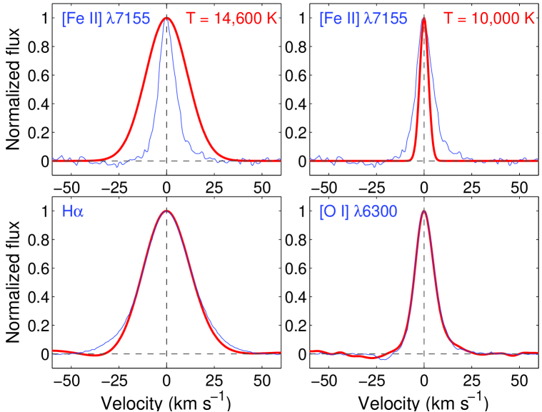
Figure 8: The upper left panel shows [Fe II] $\lambda$7155 north (blue/thin line) and a thermal (gaussian) line profile for hydrogen with a temperature of $14.6\times 10^{3}$ K (red/thick line). The lower left panel shows the result after convolving [Fe II] with the thermal component (red/thick line) vs. the observed H$\alpha$ line profile at the corresponding position (blue/thin line). The right panels show the same for [O I] $\lambda$6300, and a thermal line profile with a temperature of $10\times 10^{3}$ K for oxygen. The zero velocity corresponds to the peak flux of the lines.

4.2 The intermediate component

In Tables LABEL:tab:broadlinesN and LABEL:tab:broadlinesS we give fluxes of the intermediate line components. The table also provides velocities of the peak of the line profiles, as well as maximum red and blue velocities of the lines. All velocities are with respect to the corresponding narrow line component.

In Figs. 9 and 10 we show a selection of line profiles of different ionization stages from the intermediate component. To facilitate a comparison with other lines we have in each figure also included the line profile of the high S/N line of [O III] $\lambda$5006.8. From the figures it is apparent that the S/N varies by a large factor from the strongest lines to the weaker, which have fluxes less than a percent of the strongest. We also see that both the profile and the peak velocities differ strongly between the northern and southern components (see Sect. 4.2.3). In general, the northern component has the highest flux, and we will therefore in the following concentrate our discussion on this part.

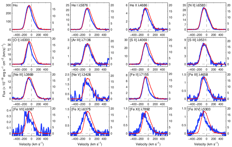
Figure 9: Line profiles of the broad emission lines (blue/thick lines) vs. [O III] $\lambda 5007$ (red/thin lines) from the northern part of the ER. The zero velocities are relative to the peak velocities of the unshocked, narrow component of the emission lines. The flux of [O III] is indicated by the right y-axis. The line profiles have been smoothed using a fourth-order Savitzky-Golay filter. Note the difference in profiles between the lower ionization lines and the coronal lines.

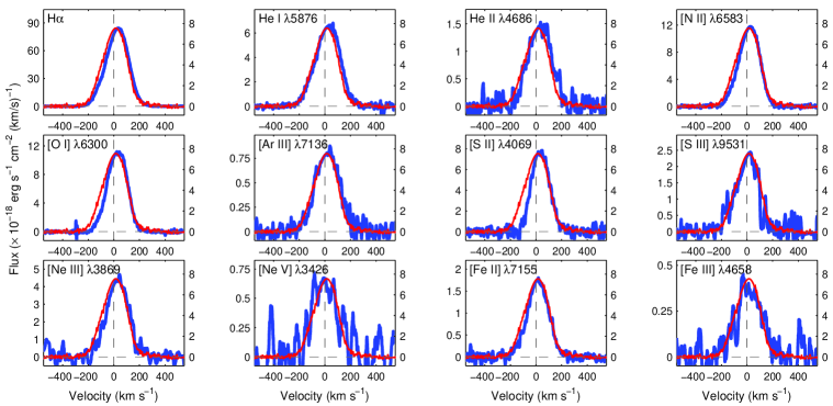
Figure 10: Line profiles of the broad emission lines (blue/thick lines) vs. [O III] $\lambda 5007$ (red/thin lines) from the southern part of the ER. The zero velocities are relative to the peak velocities of the unshocked, narrow component of the emission lines. The flux of [O III] is indicated by the right y-axis. The line profiles have been smoothed using a fourth-order Savitzky-Golay filter. Because of the low flux we do not show the coronal lines for this region.

Table 8: The dereddened Balmer line fluxes relative to H$\beta$ for the shocked gas. Only the $1\sigma$ statistical errors are given. Systematic errors are discussed in the text.

Position	H$\alpha$	H$\beta$	H$\gamma$	H$\delta$
north	$342.3\pm 0.4$	$100$	$45.13\pm 0.09$	$22.71\pm 0.07$
south	$328.6\pm 0.5$	$100$	$41.4\pm 0.2$	$19.0\pm 0.2$
Case B	$287$	$100$	$46.6$	$25.6$

4.2.1 Nebular diagnostics

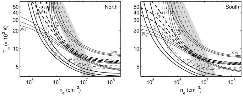
Figure 12: Electron density vs. temperature for the dereddened line ratios of emission from the shocked gas. The left panel shows the emission from the northern part of the ER and the right panel is for the southern part. The line ratios are: [O I] $\lambda\lambda 6300,6364/\lambda 5577$, [O III] $\lambda\lambda 4959,5007/\lambda 4363$, [N I] $\lambda\lambda 5198,5200/\lambda 3467$, [N II] $\lambda\lambda 6548,6583/\lambda 5755$, [S II] $\lambda\lambda 4069,4076/\lambda\lambda 6716,6731$, [S III] $\lambda\lambda 9069,9531/\lambda 6312$. Each solution curve is embraced by error curves of at least 15% to account for the systematic relative flux uncertainties. The shaded region marks the range for possible isobaric solutions. Four isobars are plotted (dashed lines) and the pressures are (in units of $10^{10}\mbox{ K}\mbox{ cm}^{-3}$): $3.9(3.1)$, $5.0(4.1)$, $6.3(5.5)$ and $7.9(7.4)$. The values in brackets are for the southern part.

As for the narrow lines in Sect. 4.1, we have used the fluxes in Tables LABEL:tab:broadlinesN and LABEL:tab:broadlinesS to probe the temperatures and the electron densities of the shocked gas. The results from our multilevel model atoms are plotted in Fig. 12. The figure panels also include shaded areas which encapsulate likely isobars (expressed in pressure units of $10^{10}$ K cm^-3). It is, as we will discuss elsewhere, a good assumption to assume constant pressure for the radiative shocks propagating into the ER. The reason we find these isobars more likely than others is that an [O III] temperature below the $\sim 10^{4}$ K typical of photoionized gas seems unlikely (marking the right boundary of shaded are), and that the [O III] temperature should be higher than the temperatures of [N II] and [S II], which roughly coincides with an [O III] temperature of $\sim 4\times 10^{4}$ K (giving the left boundary). The latter temperature is more typical of shock excitation (see next section). From Fig. 12 this temperature interval for [O III] constrains the electron density in the [O III] emitting region to be between $10^{6}-10^{7}\mbox{ cm}^{-3}$ for both the northern and southern parts of the ER.

Furthermore, Fig. 12 shows a very reasonable temperature structure of the emitting gas in the shaded area, with the temperature decreasing, in order, through the [O III], [N II]/[S III], [O I], [S II] and [N I] regions. In the [N I] region it could be as low as $(4-5)\times 10^{3}$ K, although the exact temperature depends on the degree of ionization there. For the unshocked ER we found the sequence [O III], [S III], [N II], [S II] and [O I], which would be the same also for the shocked gas if we limit ourselves to the upper densities of the shaded area in Fig. 12 where the [S III] temperature is higher than that of [N II]. However, this can only be regarded as a hint since there is no clear reason why the temperature stratification should be exactly the same in the unshocked and shocked gas.

In general our results agree with the nebular analysis performed by Pun et al. (2002), as they found roughly the same (within errors) elemental sequence of decreasing temperature. However, their data suffer from comparatively large uncertainties for some of the line ratios, making a direct comparison rather difficult. Nevertheless, we find good agreements for the [N II] and [O III] densities and temperatures. From our nebular analysis we find, however, consistently higher temperatures for [O I] than those estimated by Pun et al. (2002), although the flux ratios are similar. The origin of this is not clear.

4.2.2 Origin of the optical lines

A detailed discussion of the characteristics of the emission from the shocked gas can be found in Pun et al. (2002). Here we only discuss the points relevant to our observations.

It is easy to exclude thermal broadening as the cause of the intermediate components. A $V_{\rm FWHM}\sim 200\rm\leavevmode\nobreak\ km\leavevmode\nobreak\ s^{-1}$ would indicate a temperature of $T\sim 10^{6}$ K, and at this temperature the observed ions would be collisionally ionized. Instead, these optical emission lines of the low ionization species originate from the photoionization zone behind the radiative shock, with a temperature of $\sim 10^{4}$ K (Pun et al. 2002). It is therefore obvious that the shape of the line profiles must be dominated by the shock dynamics, rather than thermal broadening.

We have calculated models of radiative shocks for several shock velocities between 100 – 500 $\rm\leavevmode\nobreak\ km\leavevmode\nobreak\ s^{-1}$, using a shock code based on the most recent atomic data. The details of this, as well as models for the shock emission in SN 1987A, will be discussed in Fransson et al. (2007). Here we only make some general remarks about the origin of the different lines. As an example, we take the $V_{s}=300\rm\leavevmode\nobreak\ km\leavevmode\nobreak\ s^{-1}$ shock model with a pre-shock density of $10^{4}\mbox{ cm}^{-3}$, similar to that of the ER.

Immediately behind the shock the temperature for this shock velocity is $\sim 1.5\times 10^{6}$ K. This is where part of the soft X-ray lines (Zhekov et al. 2005, 2006) and the coronal lines discussed in Gröningsson et al. (2006) arise. For shock velocities in the range $V_{s}=250-400\rm\leavevmode\nobreak\ km\leavevmode\nobreak\ s^{-1}$ the thickness of this collisionally ionized, hot region is

$$D_{cool}\approx 8.5\times 10^{14}\left({n_{0}\over 10^{4}\mbox{ cm}^{-3}}\right)^{-1}\left({V_{s}\over 300\rm\leavevmode\nobreak\ km\leavevmode\nobreak\ s^{-1}}\right)^{4.4}\rm\ cm,$$ (2)

where $n_{0}$ is the electron density in the pre-shock gas, i.e., in the ER. At this point the temperature is $\sim 10^{5}$ K. The gas then undergoes a thermal instability and cools to $\sim 10^{4}$ K in a very thin region. After this the gas temperature is stabilized by photoionization heating, and a partially ionized zone takes over. In this zone the degree of ionization, $x_{e}$, and temperature decrease from $x_{e}\sim 1.0$ and $T_{e}\sim 10^{4}$ K, respectively, to very low values.

The models also show that the time for a shock to become radiative, $t_{\rm cool}$, is

$$t_{\rm cool}\approx 6.7\left({n_{0}\over 10^{4}\mbox{ cm}^{-3}}\right)^{-1}\left({V_{s}\over 300\rm\leavevmode\nobreak\ km\leavevmode\nobreak\ s^{-1}}\right)^{3.4}\rm years.$$ (3)

In the absence of a magnetic field the density in the photoionized region is

$$n_{\rm ph}\approx 10^{2}\left({V_{s}\over 100\rm\leavevmode\nobreak\ km\leavevmode\nobreak\ s^{-1}}\right)^{2}\left({T_{\rm ph}\over 10^{4}\leavevmode\nobreak\ \rm K}\right)^{-1}n_{0}\ ,$$ (4)

where $T_{\rm ph}$ is the temperature in the photoionized zone. If there is a sufficiently strong magnetic field this may limit the compression behind the shock to $\sim(8\pi\rho_{0})^{1/2}V_{s}/B_{0}$, where $\rho_{0}$ and $B_{0}$ are the density and magnetic field in the pre-shock gas, respectively (Cox 1972). For $V_{s}\sim 300\rm\leavevmode\nobreak\ km\leavevmode\nobreak\ s^{-1}$ and $n_{0}\sim 10^{4}\mbox{ cm}^{-3}$ we therefore expect a density of $\sim 10^{7}\mbox{ cm}^{-3}$, which is in good agreement with the density we infer in this region, $4\times 10^{6}-2\times 10^{7}\mbox{ cm}^{-3}$ (Sect. 4.2.1). There is therefore not from this observation any need for a dominant magnetic field.

Besides the coronal lines, also the [Ne V] lines come from the cooling, collisionally ionized region with $(1-3)\times 10^{5}$ K. In terms of emissivity, [Ne V] takes over roughly where [Fe X] drops. The [O III] and [Ne III] lines arise from a wide range of temperatures, $(2-10)\times 10^{4}$ K, in the collisionally ionized zone, but also have a contribution from the photoionized zone at $\sim 10^{4}$ K.

Both the H I and He I lines are dominated by the photoionized region just behind the cooling region at $\sim 10^{4}$ K. Most of the emission comes from the region where $x_{e}\!\!\!\phantom{\geq}\smash{\buildrel\over{\lower 2.67502pt\hbox{$\buildrel\lower 2.14001pt\hbox{$\displaystyle>$}\over{\sim}$}}}\,\,0.1$, with a thickness of only $\sim 10^{12}$ cm. The low ionization lines from [O I], [N II], [S II], and [Fe II] all come from the photoionized zone, but the emission extends to a lower temperature and ionization compared to the H I and He I lines. With the exception of the coronal lines, the optical line emission therefore require radiative shocks.

4.2.3 Line profiles

The interpretation of the shape of the line profile is not straightforward, although it is clear that it is dominated by the fluid motion behind the shocks, while thermal broadening should only have a minor influence. As discussed in Sect. 1, it is, however, likely that there is a range of shock velocities, determined by the blast-wave velocity, density and the geometry of the blobs.

Furthermore, the line profiles only reflect the projected shock velocities along the line of sight, and consequently, the FWZI velocity is only a lower limit to the maximum velocities of the radiative shocks driven into the protrusions. At this epoch (2002 October) the shocks have had about $\sim 5$ years to cool since first impact, and from the FWZI of the line profile of H${\alpha}$ (see Tables LABEL:tab:broadlinesN and LABEL:tab:broadlinesS), we estimate that shocks with velocities $\!\!\!\phantom{\leq}\smash{\buildrel\over{\lower 2.67502pt\hbox{$\buildrel\lower 2.14001pt\hbox{$\displaystyle<$}\over{\sim}$}}}\,\,260\rm\leavevmode\nobreak\ km\leavevmode\nobreak\ s^{-1}$ have had enough time to cool. This velocity depends on the density, $V_{\rm cool}\propto n_{0}^{-0.29}$. As faster shocks become radiative the maximum shock velocity resulting in radiative shocks is expected to increase with time. Therefore, the widths of the emission lines are also expected to increase.

If we compare the line profiles of the different lines we find some very interesting differences. The low ionization ions such as H$\alpha$, He I, [O III] and up to [Ne V] and [Fe VII], all have very similar profiles, with peak velocities $-60{\rm\leavevmode\nobreak\ to\leavevmode\nobreak\ }-80\rm\leavevmode\nobreak\ km\leavevmode\nobreak\ s^{-1}$, with $V_{\rm blue}\sim-260\rm\leavevmode\nobreak\ km\leavevmode\nobreak\ s^{-1}$ for the northern part of the ER (Fig. 9). The coronal lines have, however, a considerably higher peak velocity of $\sim-130\rm\leavevmode\nobreak\ km\leavevmode\nobreak\ s^{-1}$, and extend for [Fe XIV] to $V_{\rm blue}\sim-387\rm\leavevmode\nobreak\ km\leavevmode\nobreak\ s^{-1}$. This indicates that these two groups of lines do not arise from exactly the same regions.

An advantage with this comparatively early epoch is that the emission from the northern part of the ER is still dominated by Spot 1. At more recent epochs, a large number of blobs along the ER, all with different line of sight projections, contribute to the emission. There should therefore at the epoch discussed in this paper not be any serious contamination from other spots with different line-of-sight angles and shock velocities. The line profile is therefore dominated by the geometry and density distribution around the blob. Further support for this comes from more recent observations in 2005 with the SINFONI instrument at VLT (Kjaer et al. 2007). These adaptive optics observations have lower spectral resolution, but higher spatial resolution than UVES, $\sim 0\aas@@fstack{\prime\prime}2$. These observations show that even in 2005, when many blobs contribute to the emission in the ER, there is an agreement between the peak velocity of the lines in the direction of the UVES slit, as measured by SINFONI, and that obtained from the UVES observations. In contrast to our UVES observations, the SINFONI observations, do not show the full distribution of velocities, only the average at each point.

In this context we note the difference between the northern and southern line profiles shown in Figs. 9 and 10 (see also table 4 and 5). While the peak velocities, $V_{peak}$, are $-50-(-90)\rm\leavevmode\nobreak\ km\leavevmode\nobreak\ s^{-1}$ for the low and intermediate ionization lines from the northern part of the ER, they are in the range $10-40\rm\leavevmode\nobreak\ km\leavevmode\nobreak\ s^{-1}$ for the southern part. As discussed in Kjaer et al., these differences are consistent with the general geometry of the ER. Because of the low fluxes we can, however, not say much about the profiles of the coronal lines from the southern part.

When we compare the line profiles of the low ionization lines (e.g. [O I], [S II] and [Fe II]) with the intermediate ionization lines (e.g. [O III] and [S III]) we find that for the northern part the blue wings are very similiar. However, the red wings of the low ionization lines are significantly weaker compared to the intermediate ionization lines. The opposite is true for the southern part. This indicates that the excitation conditions are different in the two regions.

Pun et al. (2002) find that a simple spherical geometry well explains the basic features of the line profile from Spot 1. They, however, find it difficult to fit the wing with velocities $\la-150\rm\leavevmode\nobreak\ km\leavevmode\nobreak\ s^{-1}$ with this model, and therefore invoke a ’turbulent’ smoothing, possibly originating from instabilities in the shock structure. While this may be reasonable, it is difficult to understand how this can produce velocities higher than the shock velocity. Instead, we believe that it is more reasonable that the wings come from the highest velocity shocks, where only a small fraction of the gas, presumably that with the highest densities, has had time to cool. There should then also be a contribution from adiabatic shocks, with cooling time longer than that indicated from Eq. (3). Pun et al. (2002) suggest that these could be responsible for some of the X-ray emission observed.

This picture is supported by our observations of the larger extent of the coronal lines, up to $\sim 400\rm\leavevmode\nobreak\ km\leavevmode\nobreak\ s^{-1}$, compared to the lower ionization lines. Some of the coronal emission may therefore originate from adiabatic shocks, which are also likely to give rise to some of the soft X-ray emission seen by Chandra (Zhekov et al. 2005, 2006). If this is correct one expects the maximum velocity of both the coronal lines, and especially the low ionization lines, to increase with time.

We note that the shock velocity should be $\sim 4/3\times$ the gas velocity immediately behind the shock, as reflected in the line widths of the coronal lines. The velocity of the cool gas seen in the low ionization lines should, on the other hand, be close to that of the shock velocity. Therefore an extent of $\!\!\!\phantom{\geq}\smash{\buildrel\over{\lower 2.67502pt\hbox{$\buildrel\lower 2.14001pt\hbox{$\displaystyle>$}\over{\sim}$}}}\,\,400\rm\leavevmode\nobreak\ km\leavevmode\nobreak\ s^{-1}$ of the coronal lines indicates a shock velocity of at least $\!\!\!\phantom{\geq}\smash{\buildrel\over{\lower 2.67502pt\hbox{$\buildrel\lower 2.14001pt\hbox{$\displaystyle>$}\over{\sim}$}}}\,\,510\rm\leavevmode\nobreak\ km\leavevmode\nobreak\ s^{-1}$.

Although the emission from the coronal lines clearly comes from higher velocities than the lower ionization stages, it is important to realize that there are also in these evidence for gas at velocities considerably higher than $V_{\rm blue}$ or $V_{\rm red}$, which only gave the extension to 5% of the peak flux. In particular, the H$\alpha$ line, with the best S/N of all lines, shows clear evidence of an extension to considerably higher velocity than $V_{\rm blue}\approx-260\rm\leavevmode\nobreak\ km\leavevmode\nobreak\ s^{-1}$. To illustrate this we show in Fig. 11 H$\alpha$ on a logarithmic flux scale, From this we see that this line has a weak blue extension up to $\sim-450\rm\leavevmode\nobreak\ km\leavevmode\nobreak\ s^{-1}$, while the red extension is up to $\sim 350\rm\leavevmode\nobreak\ km\leavevmode\nobreak\ s^{-1}$.

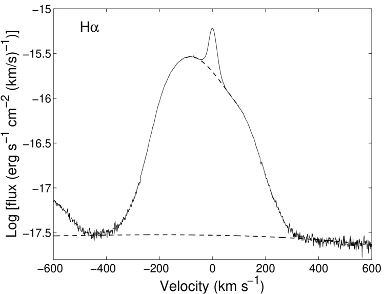
Figure 11: The narrow and intermediate components of H$\alpha$ for the northern part of the ER. The dashed lines show the estimated zero intensity levels for the narrow and intermediate components respectively. The blue wing of the intermediate component is only barely separated from the emission of [N II] $\lambda 6548$. The zero velocity corresponds to the peak flux of the narrow component.

Therefore, at least a small fraction of these high velocity shocks have time to cool. Most likely this comes from shocked gas with densities considerably higher than that typical in the ER, $\sim 10^{4}\mbox{ cm}^{-3}$. It is in this connection interesting that Lundqvist & Fransson (1996) find evidence for densities $\!\!\!\phantom{\geq}\smash{\buildrel\over{\lower 2.67502pt\hbox{$\buildrel\lower 2.14001pt\hbox{$\displaystyle>$}\over{\sim}$}}}\,\,3\times 10^{4}\mbox{ cm}^{-3}$ in the ER. From Eq. (3) we find that for a shock velocity of $450\rm\leavevmode\nobreak\ km\leavevmode\nobreak\ s^{-1}$ gas with a density of $\!\!\!\phantom{\geq}\smash{\buildrel\over{\lower 2.67502pt\hbox{$\buildrel\lower 2.14001pt\hbox{$\displaystyle>$}\over{\sim}$}}}\,\,4\times 10^{4}\mbox{ cm}^{-3}$ should have time to cool.

We finally remark that it is well known that radiative shocks in this velocity range are unstable to instabilities with wavelength of the order of the cooling length (Chevalier & Imamura 1982; Strickland & Blondin 1995; Sutherland et al. 2003). These may add further to the already complex line profiles.

5 Summary

Our UVES observations show the dynamics of the shock interaction in SN 1987A with unprecedented spectral resolution. We find evidence for shock velocities up to $\sim 500\rm\leavevmode\nobreak\ km\leavevmode\nobreak\ s^{-1}$. From the larger extent of the line profiles of the coronal [Fe X-XIV] lines compared to the low ionization lines, we argue that the highest velocities come from adiabatic shocks, which have not had time yet to cool. Shocks with velocity less than $\sim 250\rm\leavevmode\nobreak\ km\leavevmode\nobreak\ s^{-1}$ are radiative and give rise to the rest of the optical lines. We do, however, also find evidence for a minor component of radiative shocks with higher velocity. As more and more gas cools we expect the width of especially the low ionization lines to increase.

While the coronal lines and high ionization lines like [O III] and [Ne III-V] arise in the collisionally ionized hot gas behind the shocks, the low ionization lines come from gas photoionized by the shock radiation. The densities we derive from the line ratios are consistent with the large compression expected in a radiative shock.

The emission at this epoch is dominated by Spot 1. In a subsequent paper we will discuss the evolution of these lines with time as more spots emerge and the shocked gas at this epoch has had more time to cool.

Appendix A Test of flux calibration

Table 9: Comparison of fluxes from HST/STIS and UVES data sets.

Lines	Grism	Flux (ergs s-1 cm-2)		Ratio	Date of HST/STIS observations
		STIS	UVES	STIS/UVES
H${\gamma}\leavevmode\nobreak\ \lambda$4340	G430L	$1.06\times 10^{-14}$	$5.74\times 10^{-15}$	1.85	2000-11-03
[O I] $\lambda$6300	G750L	$1.20\times 10^{-14}$	$5.80\times 10^{-15}$	2.05	2000-11-03
[S II] $\lambda\lambda$4068,4076	G430L	$2.35\times 10^{-14}$	$9.83\times 10^{-15}$	2.39	2002-10-29
H${\beta}\leavevmode\nobreak\ \lambda$4861	G430L	$7.19\times 10^{-14}$	$2.73\times 10^{-14}$	2.63	2002-10-29
[N II] $\lambda$5755	G750L	$2.44\times 10^{-14}$	$1.01\times 10^{-14}$	2.41	2002-10-29
He I $\lambda$7065	G750L	$7.59\times 10^{-15}$	$3.56\times 10^{-15}$	2.13	2002-10-29

To test our flux calibration of the UVES spectra, we downloaded archival HST/STIS data for two epochs: 2000 November 3 and 2002 October 29. The epochs are close to our UVES data from 2000 December $9-14$ (discussed in Gröningsson et al. 2007 in prep.) and 2002 October $4-7$ (discussed in this paper). The STIS observations are long-slit spectroscopy observations made with the first-order gratings G430L and G750L which cover the spectral intervals $2900-5700$ Å (resolution 2.73 Å pixel^-1) and $5250-$10 300 Å (resolution 4.92 Å pixel^-1), respectively. The aperture was $52\arcsec\times 2\arcsec$, and the slit was placed so that it covers half of the ring, with the dispersion direction in the north-south direction. A second set of observations were made for the other half of the ring. One therefore obtains separate spectra for the northern and southern parts of the ring of SN 1987A. These have to be added together to get the total ring flux. There is a marginal spatial overlap between the two sets of observations, but this is small enough (i.e., a few per cent) to be unimportant for our test.

The pipeline-reduced STIS spectra have several cosmic rays, but there are fortunately “clean” lines in most parts of the spectrum so that we can test the flux calibration for the various spectral settings of UVES. The lines we chose in the red part of the spectrum (G750L) are [N II] $\lambda$5755, [O I] $\lambda$6300 and He I $\lambda$7065, and in the blue (G430L) we selected [S II] $\lambda\lambda$4068,4076, H$\gamma$ and H$\beta$.

To obtain the flux of a particular line in the STIS spectrum, we first manually cleaned the region around the line from cosmic rays. We then integrated the spectrum in the dispersion direction for each spatial row that cuts across the ring. With the pixel scale of STIS, this means that we made spectral scans for up to 37 spatial rows (the exact number depends on the brightness of the ring for the line analyzed) to cover each of the full half ring. We then summed up the flux from all the rows in the spectrum and added the flux from the opposite side of the ring to get the total ring flux for each line.

As the spectral resolution of STIS does not allow us to separate the narrow component from the intermediate-velocity component, the flux estimate from STIS is a sum of both these components. The STIS data do, however, allow us to separate out any underlying continuum. For the UVES spectra we therefore integrated the emission in the narrow plus intermediate velocity component to make a direct comparison with the STIS flux.

The STIS fluxes for the whole ring and ratios of STIS to UVES fluxes are summarized in the Table 9. The fact that the STIS flux is higher than the UVES flux is reasonable since the UVES slit only encapsulates part of the ring whereas the STIS flux is for the full ring. The ratio of STIS/UVES flux appears to be somewhat lower for 2000 November ($\sim 2.0$) than for 2002 October ($\sim 2.4$). This could be due to temporal flux variations round the ring (e.g., new spots appearing between 2000 and 2002), or may be due to a systematic error in the fluxing of the UVES spectra. The former is not unlikely since Spot 1, encapsulated by the UVES aperture, dominates the ring interaction emission in the 2000 November data, whereas two years later, it is less dominant and various parts (also those outside the UVES slit) contribute to the ring interaction emission. Because the STIS/UVES flux ratio does not show any obvious wavelength-dependent trends (see Table 9), a constant multiplicative factor can be used for the UVES spectrum to estimate the total flux from the full ring. As we have discussed, the factor may be somewhat different for different epochs. As we here concentrate on our UVES data from 2002 October, we have chosen the factor 2.4 for this epoch.

To check the significance of the multiplicative factor, we downloaded HST/WFPC2 archival data from 2002 May 10 obtained using the F656N filter. The pivot wavelength for this filter is 6563.8 Å and the band width is 53.8 Å. We convolved the image with a 2D Gaussian function to simulate the seeing of our UVES data. We tested three FWHM values of the Gaussian: 0$\aas@@fstack{\prime\prime}$6, 0$\aas@@fstack{\prime\prime}$8 and 1$\aas@@fstack{\prime\prime}$0. The Gaussian was truncated at 5$\arcsec$ as the inclusion of emission outside this radius did not change the results. Figure 13 shows the original and a blurred image, simulating 0$\aas@@fstack{\prime\prime}$8 seeing, with the 0$\aas@@fstack{\prime\prime}$8 UVES slit overlaid on top of them. The total flux from the ring was assumed to be the flux within the larger box in the original image. (The contributions from the ejecta and outer rings are low in comparison with that of the inner ring.) We then formed a ratio of emission through the 0$\aas@@fstack{\prime\prime}$8 slit and the total emission from the ring. The results are shown in the Table 10.

For the original image (i.e., no seeing), no emission from the north-west and south-east parts of the ring enters the 0$\aas@@fstack{\prime\prime}$8 slit. With increased “seeing” emission from these parts ventures into the slit, whereas emission within the slit in the original image falls outside the slit. According to Table 10 the “loss” of flux measured through the slit is slightly larger than the “gain” since the ratio (total flux to UVES slit flux) increases with the degree of blurring. The effect is, however, rather small, with the flux within the UVES slit decreasing from 43.7% to 40.8% with seeing increasing from 0$\aas@@fstack{\prime\prime}$6 to 1$\aas@@fstack{\prime\prime}$0. This means that seeing effects have no major impact on the absolute fluxing of the UVES spectra, and that spectra obtained under different seeing conditions can be coadded without introducing systematic error in the fluxing. Also, since the ratios in Table 10 show very good agreement with the ratio of 2.4 obtained from the comparison between UVES and STIS fluxes, we are confident in the magnitude of this factor. The main effect of seeing is a redistribution of flux into and out from the area covered by the slit. For a time series of spectra it therefore makes sense to compare spectra with roughly the same average seeing to study changes of physical properties of the ring.

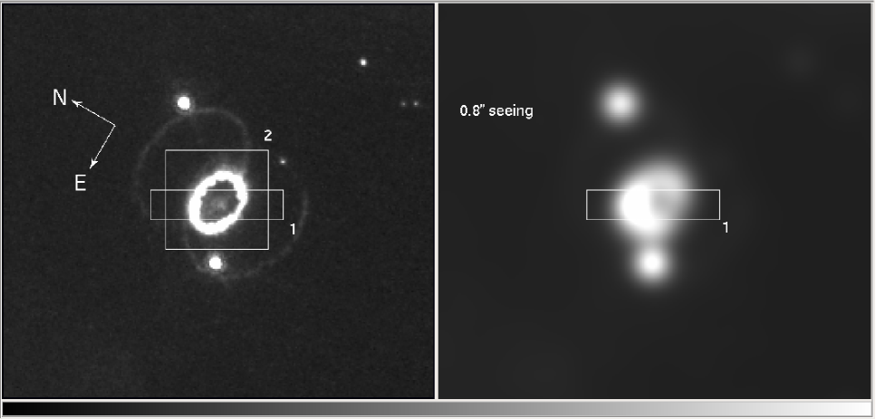
Figure 13: H$\alpha$ image of SN 1987A obtained with HST/WFPC2 in 2002 May 10 using the narrow F656N filter centered at the rest wavelength of H$\alpha$. The rectangular boxes are apertures which were chosen to model UVES data (marked “1”) and STIS data (marked “2”). The image to the left is unconvolved. The other image is smoothed using 2D Gaussian functions and represent a seeing of 0$\aas@@fstack{\prime\prime}$8. The lower flux cut in both images are roughly at the flux level of the outer rings in the image to the right. As the inner ring is nearly two orders of magnitude brighter (cf. Fig. 1) and the flux from Stars 2 and 3 fall below this flux cut at the position of the UVES slit, these stars have no important influence on the flux calibration. Note the dominance of Spot 1 in the north-east part of the ring.

Table 10: Comparison of fluxes from HST/STIS and UVES data sets using HST/WFPC2 with F656N filter centered at the rest wavelength of H$\alpha$. The apertures shown on the Figure 13.

Modeled seeing	Ratio of aperture “2” to “1”
unblurred	2.31
0$\aas@@fstack{\prime\prime}$6	2.29
0$\aas@@fstack{\prime\prime}$8	2.35
1$\aas@@fstack{\prime\prime}$0	2.45