Fast 2D non–LTE radiative modelling of prominences

Abstract

Context. New high-resolution spectropolarimetric observations of solar prominences require improved radiative modelling capabilities in order to take into account both multi-dimensional – at least 2D – geometry and complex atomic models.

Aims. This makes necessary the use of very fast numerical schemes for the resolution of 2D non–LTE radiative transfer problems considering freestanding and illuminated slabs.

Methods. The implementation of Gauss-Seidel and successive over-relaxation iterative schemes in 2D, together with a multi-grid algorithm, is thoroughly described in the frame of the short characteristics method for the computation of the formal solution of the radiative transfer equation in cartesian geometry.

Results. We propose a new test for multidimensional radiative transfer codes and we also provide original benchmark results for simple 2D multilevel atom cases which should be helpful for the further development of such radiative transfer codes, in general.

1 Introduction

Efficient iterative schemes have been introduced in the field of two-dimensional (2D) non-LTE numerical radiative transfer during the last, say, fifteen years. These developments most often rely on the combination of the short characteristics (SC) method for the so-called formal solution of the radiative transfer equation (in cartesian geometry see e.g., Kunasz & Auer sc2 (1988), Auer & Paletou lhafp (1994) and in various other geometries, van Noort et al. vanoort (2002)) and efficient iterative schemes such as Gauss-Seidel and successive over-relaxation (GS/SOR) iterative processes (Trujillo Bueno & Fabiani Bendicho tf1 (1995), Paletou & Léger paleg (2007)) together with multi-grid (MG) methods (Auer et al. lhaft (1994), Fabiani Bendicho et al. fta2 (1997)).

Hereafter, we are interested in a more realistic modelling of isolated and illuminated structure, such as prominences hanging in the solar corona (see e.g., Paletou fp95 (1995), fp96 (1996)). Our future work will emphasis on the synthesis of the H and He spectra. Indeed, the most recent modelling efforts concerning the synthesis of the H and He spectrum in prominences has been performed using either mono-dimensional (1D) slabs (Labrosse & Gouttebroze lagou1 (2001), lagou2 (2004)), or using 2D cartesian slabs in magnetohydrostatic equilibrium and the Multilevel Accelerated Lambda Iteration (MALI) technique for the solution of the non–LTE transfer problem (Heinzel & Anzer phua1 (2001), phua2 (2005)). Concerning the spectrum of H, Gouttebroze (2006) also presented promising new results using 2D cylindrical models of coronal loops.

Our primary aim is thus to improve diagnostics based, in particular, on He i lines by treating a detailed He-atomic model including the atomic fine structure together with 2D non-LTE radiative transfer. We are motivated here by new solar prominences observations (see e.g., Paletou et al. paletal (2001), Merenda et al. laura (2006)) which also triggered some revisions of inverting tools (López Ariste & Casini lopcas (2002)). And up to now, the later diagnostic tools are limited to the assumption that the relevant (observed) He spectral lines are optically thin; it is, however, easy to check from high spectral resolution observations that a spectral line like $D_{3}$ of He i in the visible, for instance, is not always optically thin, even in quiescent prominences (Landi Degl’Innocenti landi82 (1982), López Ariste & Casini lopcas (2002)). Furthermore, the expected optical thicknesses of 1 to 10 say, in such structures let us forecast the presence of significant geometrical effects on the mechanism of formation of this spectral line, as the ones already put in evidence on H$\alpha$ by Paletou (fp97 (1997)).

The combination of 2D geometry with a very detailed atomic model for He obviously requires a more efficient radiative transfer code as compared to the one developed from the MALI method by Paletou (1995). And clearly enough, the planned improvement of the radiative modelling including multidimensional geometry together with multi-level, realistic atomic models have to rely on those new and fast radiative transfer methods based on GS/SOR with multigrid numerical schemes.

GS/SOR methods, best implemented within a short characteristics formal solver, have been described in every details by Trujillo Bueno & Fabiani Bendicho (tf1 (1995)) but only in the frame of the two-level atom case and in 1D geometry. In another article, Fabiani Bendicho et al. (fta2 (1997)) have nicely described the implementation of non-linear multi-grid techniques, using an efficient iterative method such as a GS/SOR scheme. However, they just did not describe the implementation of, 1D or multidimensional, multilevel GS/SOR scheme using the SC method. Besides, Paletou & Léger (paleg (2007)) have finally made explicit the implementation of GS/SOR iterative schemes in the multi-level atom case, restricted though to a 1D plane-parallel geometry.

The present article aims therefore at “filling the gap” by providing all the elements required for a successful implementation of a GS/SOR iterative scheme in a 2D cartesian geometry. In order to do so, we adopt the line of detailing the method in the frame of the 2-level atom given that our detailed description of the multilevel strategy published elsewhere (Paletou & Léger paleg (2007)) does not need to be commented any further for the jump from 1D to 2D. Therefore, we also provide hereafter various benchmark results for the 2D-multilevel atom case, still unpublished to date, using simple atomic models taken from Avrett (avrett (1968); see also Paletou & Léger paleg (2007)). Moreover, an original comparison between 2D numerical results and independent analytical solutions is made.

We shall recall in §2 the basic principles of ALI and GS/SOR iterative schemes in the frame of a two-level atom model and in 1D geometry. Then in §3 we shall describe, in details, how the GS/SOR numerical method can be implemented for the case of 2D slabs in cartesian geometry, therefore upgrading the 2D short characteristic method initially published by Auer & Paletou (lhafp (1994)). A new test for numerical radiation transfer codes is briefly presented in §4. Then we shall finally present, in §5, benchmark results for simplified multilevel atomic models in 2D geometry and some illustrative examples clearly demonstrating in which conditions geometrical effects should be seriously considered.

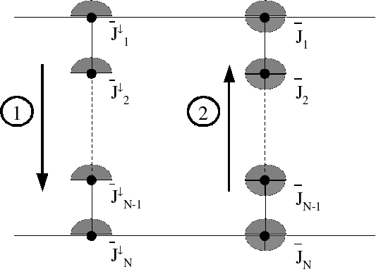
Figure 1: Schematic view of the short characteristics method for the computation of $\bar{J}$ in a 1D grid of $N$ points in the case of a ALI iterative scheme. During the first (downward here) pass the angular integration as in Eq. (2) is made over half an hemisphere; it is completed during the 2nd (upward) pass, allowing for the source function update according to Eq. (1).

2 Gauss-Seidel and SOR iterative schemes basics

In the two-level atom case, the non-LTE line source function, assuming complete redistribution in frequency, is usually written as

$$S(\tau)=(1-\varepsilon)\bar{J}(\tau)+S^{*}(\tau)\,,$$ (1)

where $\tau$ is the optical depth, $S^{*}$ is the thermal source function and $\varepsilon$ is the collisional destruction probability; unless explicitly mentioned, $S^{*}=\varepsilon B$, where $B$ is the Planck function. $\bar{J}$ is the usual mean intensity defined as

$$\bar{J}=\oint\displaystyle{{{d\Omega}\over{4\pi}}}\int_{0}^{\infty}{\phi_{\nu}I_{\nu\Omega}d\nu}\,,$$ (2)

where the optical depth dependence has been omitted for the sake of simplicity; as usual, $I_{\nu\Omega}$ is the specific intensity and $\phi_{\nu}$ is the line absorption profile. Usually again, the mean intensity is written as the formal solution of the radiative transfer equation i.e.,

$$\bar{J}=\Lambda[S]\,.$$ (3)

Following the Jacobi-type iterative scheme introduced in numerical transfer by Olson et al. (oab (1986)), we shall consider a splitting operator $\Lambda^{\ast}$ equal to the exact diagonal of the true operator $\Lambda$. Now introducing the perturbations

$$\left\{\begin{array}[]{lll}\Lambda&=&\Lambda^{\ast}\,+\,(\Lambda\,-\,\Lambda^{\ast})\\ S^{\mathrm{(new)}}&=&S^{\mathrm{(old)}}\,+\,\delta S\\ \end{array}\right.$$ (4)

in Eq. (1), we are led to an iterative scheme such that

$$S^{\mathrm{(new)}}=[1\,-\,(1\,-\,\varepsilon)\Lambda^{\ast}]^{-1}\{(1\,-\,\varepsilon)(\Lambda\,-\,\Lambda^{\ast})S^{\mathrm{(old)}}\,+\,\varepsilon B\}\,.$$ (5)

Running the later scheme to convergence is better known in numerical radiative transfer as the “ALI method”. As schematized in Fig. 1, using the short characteristics method in 1D geometry (Olson & Kunasz sc1 (1987), Kunasz & Auer sc2 (1988)), the formal solution is obtained by sweeping the grid say, first in directions $-\Omega$ ($\mu<0$) i.e., from the surface down to the bottom of the atmosphere, and then in the opposite, upward directions $+\Omega$ ($\mu>0$) starting from the bottom of the atmosphere up to its surface though. The specific intensity $I_{\nu\Omega}$ is then advanced step by step during each pass, partially integrated over angles and frequencies during the downward pass while, during the second (upward) pass, completion of the angular integration allows for the full determination of the mean intensity $\bar{J}_{k}$ at each depth $\tau_{k}$ of the 1D grid and, finally, to the update of the source function

$$S_{k}^{\mathrm{(new)}}=S_{k}^{\mathrm{(old)}}\,+\,\Delta S_{k}\,,$$ (6)

on the basis of increments such that

$$\Delta S_{k}={{(1-\varepsilon)\bar{J}_{k}^{\mathrm{(old)}}+\varepsilon B_{k}-S_{k}^{\mathrm{(old)}}}\over{1-(1-\varepsilon)\Lambda_{kk}}}\,,$$ (7)

where $\Lambda_{kk}$ is a scalar equal to the diagonal element of the full operator $\Lambda$ at such a depth in the atmosphere and where superscripts (old) denote quantities already known from the previous iterative stage.

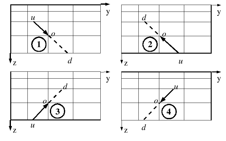
Figure 2: The 2D grid is swept four times: first pass in directions $\searrow$ defined in panel 1, second pass in directions $\nwarrow$ defined in panel 2, third pass in directions $\nearrow$ defined in panel 3 and fourth pass in directions $\swarrow$ defined in panel 4. Sweeping must be done away from the boundaries so that upwind intensities – see Eq. (11) – are always known.

For a Gauss-Seidel iterative scheme, the sweeping of the atmosphere is identical but as soon as the mean intensity $\bar{J}_{k}$ is fully computed at depth-point $k$ in the atmosphere during the upward pass, the local source function is updated immediately i.e., before completion of the 2nd pass, using increments which have now turned into

$$\Delta S_{k}^{\mathrm{(GS)}}={{(1-\varepsilon)\bar{J}_{k}^{\mathrm{(old\,and\,new)}}+\varepsilon B_{k}-S_{k}^{\mathrm{(old)}}}\over{1-(1-\varepsilon)\Lambda_{kk}}}\,,$$ (8)

where the quantity $\bar{J}_{k}^{\mathrm{(old\,and\,new)}}$ means that at the spatial point $k$ the mean intensity has to be calculated via a formal solution of the transfer equation using the “new” source function values ${S}_{j}^{\mathrm{(new)}}$ already obtained at points $j=\mathrm{ND},\ldots,(k+1)$ and the “old” source function values ${S}_{j}^{\mathrm{(old)}}$ at points $j=k,\,(k-1),\ldots,1$.

Finally, as a next step SOR iterations can simply be implemented using

$$\Delta S_{k}^{\mathrm{(SOR)}}=\omega\Delta S_{k}^{\mathrm{(GS)}}\,,$$ (9)

where $\omega$ is an overrelaxation parameter such that $1<\omega<2$. For two-level atom models in 1D, this method was originally proposed by Trujillo Bueno & Fabiani Bendicho (tf1 (1995)).

3 The 2D-cartesian geometry case

Hereafter, we shall describe in every details how the GS/SOR numerical method can be implemented for the case of 2D freestanding slabs modeled in cartesian geometry.

3.1 SC in 2D: an overview

We shall initially follow and therefore upgrade the formal solver of reference proposed originally by Kunasz & Auer (sc2 (1988)) and modified by Auer & Paletou (lhafp (1994)).

Using SC in 2D geometry, the formal solution is obtained by sweeping the grid four times, as schematized in Fig. 2, say first increasing $y$ and $z$ i.e., along directions $\Omega_{1}$ (note that $z=0$ is the surface of the atmosphere), second decreasing $y$ and $z$ along directions $\Omega_{2}$, third increasing $y$ and decreasing $z$ along directions $\Omega_{3}$, and finally decreasing $y$ and increasing $z$ along directions $\Omega_{4}$. The specific intensity $I_{\nu\Omega}$ is therefore advanced step by step during each pass, partially integrated over angles, quadrant after quadrant, and over frequencies during the first three passes while, during the fourth pass, the mean intensity $\bar{J}$ can be fully computed, completing therefore the numerical evaluation of the formal solution

$$\bar{J}_{(i,j)}=\Lambda_{(i,j)}[S]\,.$$ (10)

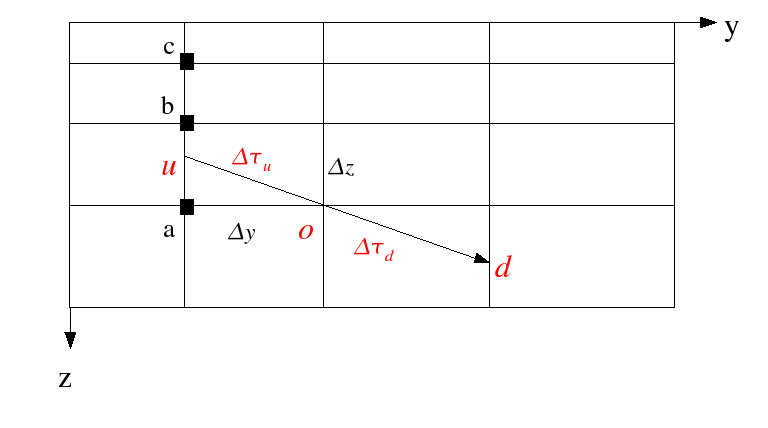
Figure 3: Example of a short characteristic across a 2D cartesian grid at depth point $o$ ($i,j$) for a ray propagating along directions $\searrow$ defined in panel 1 of Fig. 2: three points $a$, $b$ and $c$ are used for monotonic parabolic interpolation in $z$, in order to evaluate quantities at point $u$ following Auer & Paletou (lhafp (1994)).

Except at the boundary surfaces where the incident radiation is known a priori, along each direction the specific intensity at the inner grid points is advanced depth after depth. As displayed in Fig. 3, the short characteristic starts at grid point $o$ ($i,j$) and extend in the “upwind” and “downwind” directions until it hits one of the cell boundaries either at point $u$ or at point $d$ that is, not grid points in general. The specific intensity is therefore computed, according to Kunasz & Auer (sc2 (1988)), as

$$I_{o}=I_{u}e^{-\Delta\tau_{u}}+\Psi_{u}S_{u}+\Psi_{o}S_{o}+\Psi_{d}S_{d}\,.$$ (11)

where the first part of the right-hand side of this expression corresponds to the part transmitted from the “upwind” point $u$ down to the current point $o$, and the three last terms result from the analytic integration of

$${\cal{I}}=\int_{0}^{\Delta\tau_{u}}{S(\tau)e^{-\tau}}d\tau$$ (12)

along the short characteristic going from $u$ to $o$; expressions for the $\Psi$’s can be found in Paletou & Léger (paleg (2007)).

As shown in Fig. 3, in 2D geometry, $I_{u}$, $S_{u}$ and $S_{d}$ are not grid points, and they must be evaluated by interpolation on the basis of a set of grid point. In order to do so, one has first to determine on which axis, $y$ or $z$, the upwind and downwind points shall lie. We introduce $c_{y}$ (respectively $c_{z}$) the cosine between the direction into which the photon is moving and the $y$-axis (respectively the $z$-axis), $\Delta y$ the $y$ length of the cell containing both $u$ and $o$ grid points, and $\Delta z$ its length in $z$. If

$$\frac{\Delta y}{c_{y}}<\frac{\Delta z}{c_{z}}$$

the ray hits the $y$-axis and $\Delta\tau_{u}={\Delta z}/{c_{z}}$.

Following Auer & Paletou (lhafp (1994)), $I_{u}$ and $S_{u}$ are determined by interpolation along the upwind grid-line passing through points $a$ and $b$. To perform a parabolic interpolation, we shall therefore use three grid points $a$, $b$ and $c$ as displayed in Fig. 3, and where “quantities” have already been updated; along $z$-lines, interpolation weights would be given by

$$\left\{\begin{array}[]{l}\omega_{a}=\frac{\displaystyle(z_{b}-z)(z_{c}-z)}{\displaystyle(z_{b}-z_{a})(z_{c}-z_{a})}\\ \\ \omega_{b}=\frac{\displaystyle(z_{a}-z)(z_{c}-z)}{\displaystyle(z_{a}-z_{b})(z_{c}-z_{b})}\\ \\ \omega_{c}=\frac{\displaystyle(z_{a}-z)(z_{b}-z)}{\displaystyle(z_{a}-z_{c})(z_{b}-z_{c})}\end{array}\right.$$ (13)

and similar weights should be used for interpolation in $y$, using grid points ($i-1$,$j$), ($i-1$,$j-1$) and ($i-1$,$j-2$) though. Then, we are able to calculate the upwind specific intensity as

$$I_{u}=\omega_{a}I_{a}+\omega_{b}I_{b}+\omega_{c}I_{c}$$ (14)

where specific intensity values have already been computed at grid points $a$, $b$ and $c$. This is guaranteed by sweeping the grid away from one of the upwind boundaries. Note also that $S_{u}$ and $S_{d}$ are also evaluated from ($S_{a}$, $S_{b}$, $S_{c}$) using similar expressions.

For the sake of accuracy and in order to avoid the generation of spurious upwind intensities by high-order interpolation, one must use a monotonic interpolation i.e., set $I_{u}$ (and $I_{d}$) equal to the minimum or maximum of $I_{a}$ and $I_{b}$ if the parabolic interpolant lies outside the interval [min($I_{a}$,$I_{b}$), max($I_{a}$,$I_{b}$)], as proposed by Auer & Paletou (lhafp (1994)).

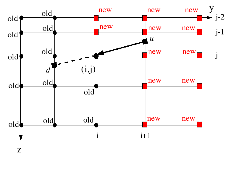
Figure 4: Let $i$ be the index along the $y$-axis and $j$ along the $z$-axis; we consider the specific intensity evaluation at any inner grid point ($i$,$j$) during the fourth pass in the 2D grid, corresponding to the directions $\Omega_{4}$ defined in Fig. 2. At this stage, all “new” grid points have already been swept, so that source functions at these points have been updated too.

3.2 Implementation of GS/SOR in 2D

Assume that one has already swept the grid three times as described in Fig. 2. By analogy with the GS/SOR numerical strategy in 1D geometry, we are now going to update the source function at each grid point during the fourth pass of the SC-2D scheme, according to the correction given in Eq. (8) and before passing to the next depth point. It is a quite straightforward task at the boundary surfaces since the incident radiation field is known a priori from the (given) external conditions of illumination.

We shall hereafter describe what has to be done at the inner grid points. Fig. 4 describes the situation once arriving at ($i$,$j$) after the 2D grid was swept thrice. Using superscripts defined in Fig. 2, the current specific intensity comes from

$$I_{(i,j)}^{\swarrow}=I_{u}^{\swarrow}e^{-\Delta\tau_{u}^{\swarrow}}+\Psi_{u}^{\swarrow}S_{u}^{\swarrow\mathrm{(new)}}+\Psi_{0}^{\swarrow}S_{0}^{\swarrow\mathrm{(old)}}+\Psi_{d}^{\swarrow}S_{d}^{\swarrow\mathrm{(old)}}\,,$$ (15)

where one must understand quantities with superscripts $\mathrm{(new)}$ such as resulting from interpolations along upwind grid lines, using source functions that has been obtained during the preceding steps. Indeed, using an expression similar to the one in Eq. (14), for an interpolation along the $z$-axis, we would have

$$S_{u}^{\swarrow\mathrm{(new)}}=\omega_{a,(i,j)}^{\swarrow}S_{(i+1,j)}^{\mathrm{(new)}}+\omega_{b,(i,j)}^{\swarrow}S_{(i+1,j-1)}^{\mathrm{(new)}}+\omega_{c,(i,j)}^{\swarrow}S_{(i+1,j-2)}^{\mathrm{(new)}}\,.$$ (16)

Before integrating over all frequencies and over the angles corresponding to the $\Omega_{4}$ directions in order to obtain the partial mean intensity

$$\bar{J}^{\swarrow}=\int_{\Omega_{4}}\frac{d\Omega}{4\pi}\int_{\nu}{\phi_{\nu}I_{\nu\Omega}d\nu}\,,$$ (17)

we shall have to correct the specific intensity calculated during the first three passes for consistency with the source function updates. More specifically, the term $I_{(i,j)}^{\nearrow}$ was calculated during the third pass as

$$I_{(i,j)}^{\nearrow}=I_{u}^{\nearrow}e^{-\Delta\tau_{u}^{\nearrow}}+\Psi_{u}^{\nearrow}S_{u}^{\nearrow\mathrm{(old)}}+\Psi_{0}^{\nearrow}S_{0}^{\nearrow\mathrm{(old)}}+\Psi_{d}^{\nearrow}S_{d}^{\nearrow\mathrm{(OLD)}}$$ (18)

using $S_{d}^{\nearrow\mathrm{(OLD)}}$ instead of the new value $S_{d}^{\nearrow\mathrm{(new)}}$ obtained from the interpolation using the updated points ($i+1$,$j$), ($i+1$,$j-1$) and ($i+1$,$j-2$) as shown in Fig. 4 since we have the identity $S_{d}^{\nearrow}=S_{u}^{\swarrow}$ ; a correcting term

$$\Delta\bar{J}_{(i,j)}^{\nearrow}=\int_{\Omega_{3}}\frac{d\Omega}{4\pi}\int_{\nu}\phi_{\nu}\left[S_{u,\nu}^{\swarrow\mathrm{(new)}}-S_{d,\nu}^{\nearrow\mathrm{(old)}}\right]\,\Psi_{d,\nu}^{\nearrow}d\nu$$ (19)

must therefore be added to the the total mean intensity by integrating the specific intensity correction over frequencies and over all angles $\Omega_{3}$ – see Fig. 2; this step is equivalent to the computation of the $\Delta J_{k}^{\mathrm{in}}$ correction mentioned by Trujillo Bueno & Fabiani Bendicho (tf1 (1995)) in their Eq. (39).

Table 1: Computation time (for a Pentium-4 @ 3 GHz processor) and number of iterations for the H i multilevel benchmark model of Avrett (1968) in a 2D grid with $y_{max}=5\,000$ km and $z_{max}=30\,000$ km together with 3 angles per octant and 8 frequencies; the temperature of the atmosphere is 5 000 K and the gas pressure $p_{g}\,=\,1\,\mathrm{dyn\,cm^{-2}}$.

Points number	MALI 2D	GSM 2D	SOR 2D	MG 2D	$R_{c}$
123x123	3min9s (46)	2min19s (29)	1min17s (16)	55s (11)	$1.1\times 10^{-2}$
163x163	9min39s (79)	6min56s (48)	3min33s (24)	1min52s (13)	$2.1\times 10^{-3}$
203x203	22min47s (116)	14min36s (68)	7min34s (33)	2min50s (14)	$5.7\times 10^{-4}$
243x243	45min32s (158)	29min10s (90)	14min3s (43)	4min13s (14)	$1.9\times 10^{-4}$

The two other terms $I_{(i,j)}^{\searrow}$ and $I_{(i,j)}^{\nwarrow}$ calculated during the first and the second passes are also still inconsistent with the last source function updates because they were calculated as

$$\begin{array}[]{llll}I_{(i,j)}^{\searrow}&=&&I_{u}^{\searrow\mathrm{(OLD)}}e^{-\Delta\tau_{u}^{\searrow}}+\Psi_{u}^{\searrow}S_{u}^{\searrow\mathrm{(OLD)}}\\ \\ &&+&\Psi_{0}^{\searrow}S_{0}^{\searrow\mathrm{(old)}}+\Psi_{d}^{\searrow}S_{d}^{\searrow\mathrm{(OLD)}}\,,\end{array}$$ (20)

and

$$\begin{array}[]{llll}I_{(i,j)}^{\nwarrow}&=&&I_{u}^{\nwarrow\mathrm{(OLD)}}e^{-\Delta\tau_{u}^{\nwarrow}}+\Psi_{u}^{\nwarrow}S_{u}^{\nwarrow\mathrm{(OLD)}}\\ \\ &&+&\Psi_{0}^{\nwarrow}S_{0}^{\nwarrow\mathrm{(old)}}+\Psi_{d}^{\nwarrow}S_{d}^{\nwarrow\mathrm{(OLD)}}\,,\end{array}$$ (21)

where we have the following identities $S_{u}^{\searrow\mathrm{(OLD)}}=S_{d}^{\nwarrow\mathrm{(OLD)}}$ and $S_{d}^{\searrow\mathrm{(OLD)}}=S_{u}^{\nwarrow\mathrm{(OLD)}}$.

These (OLD) source functions could now be calculated using updated values. For example the new value $S_{u}^{\searrow\mathrm{(new)}}=S_{d}^{\nwarrow\mathrm{(new)}}$ is obtained from an equation similar to Eq. (14) with an interpolation along $y$-axis using $S_{i,j-1}^{\mathrm{(new)}}$ – and one can see, using Fig. 4, that ($i$,$j-1$) is a “new” grid point whereas ($i-1$,$j-1$) and ($i-2$,$j-1$) are “old” grid points i.e.,

$$S_{u}^{\searrow\mathrm{(new)}}=\omega_{a,(i,j)}^{\searrow}S_{(i,j-1)}^{\mathrm{(new)}}+\omega_{b,(i,j)}^{\searrow}S_{(i-1,j-1)}^{\mathrm{(old)}}+\omega_{c,(i,j)}^{\searrow}S_{(i-2,j-1)}^{\mathrm{(old)}}$$ (22)

Similarly, the new value $S_{d}^{\searrow\mathrm{(new)}}=S_{u}^{\nwarrow\mathrm{(new)}}$ is obtained using an interpolation along $y$-axis, for instance, involving $S_{i+1,j+1}^{\mathrm{(new)}}$ and $S_{i+2,j+1}^{\mathrm{(new)}}$ – with this time, using Fig. 4, grid points at ($i+1$,$j+1$) and ($i+2$,$j+1$) are “new” whereas ($i$,$j+1$) is an “old” grid point i.e.,

$$S_{d}^{\searrow\mathrm{(new)}}=\omega_{a,(i,j)}^{\searrow}S_{(i,j+1)}^{\mathrm{(old)}}+\omega_{b,(i,j)}^{\searrow}S_{(i+1,j+1)}^{\mathrm{(new)}}+\omega_{c,(i,j)}^{\searrow}S_{(i+2,j+1)}^{\mathrm{(new)}}$$ (23)

By analogy, old specific intensities $I_{u}^{\searrow\mathrm{(OLD)}}$ and $I_{u}^{\nwarrow\mathrm{(OLD)}}$ must be updated to obtain new values calculated with interpolations using “new” grid points.

We shall then have to calculate two other corrections $\Delta J_{(i,j)}^{\searrow}$ and $\Delta J_{(i,j)}^{\nwarrow}$ by integrating these corrected specific intensities over frequencies and over directions $\Omega_{1}$ and $\Omega_{2}$, following an equation similar to Eq. (19). Finally we shall add three correcting terms to compute the correct total mean intensity at the current grid point ($i$,$j$):

$$\begin{array}[]{llll}\bar{J}_{(i,j)}&=&&\bar{J}_{(i,j)}^{\searrow}\,+\,\bar{J}_{(i,j)}^{\nwarrow}\,+\,\bar{J}_{(i,j)}^{\nearrow}\,+\,\bar{J}_{(i,j)}^{\swarrow}\\ \\ &&+&\,\Delta\bar{J}_{(i,j)}^{\nearrow}\,+\,\Delta\bar{J}_{(i,j)}^{\searrow}\,+\,\Delta\bar{J}_{(i,j)}^{\nwarrow}\end{array}\,.$$ (24)

Then it is straightforward to update the local source function $S_{i,j}^{\mathrm{(new)}}$ via Eq. (8).

However, before advancing to the next depth point ($i$,$j+1$), it is important to add the following corrections to the specific intensities of the three first passes, due to the source function update which has just been made at the current depth point :

$$\left\{\begin{array}[]{l}\Delta I_{(i,j)}^{\swarrow}=\Psi_{0}^{\swarrow}\left[S_{(i,j)}^{\mathrm{(new)}}\,-\,S_{(i,j)}^{\mathrm{(old)}}\right]\\ \\ \Delta I_{(i,j)}^{\searrow}=\Psi_{0}^{\searrow}\left[S_{(i,j)}^{\mathrm{(new)}}\,-\,S_{(i,j)}^{\mathrm{(old)}}\right]\\ \\ \Delta I_{(i,j)}^{\nwarrow}=\Psi_{0}^{\nwarrow}\left[S_{(i,j)}^{\mathrm{(new)}}\,-\,S_{(i,j)}^{\mathrm{(old)}}\right]\end{array}\right.$$ (25)

This last stage is analogous to the correction described by Trujillo Bueno & Fabiani Bendicho (tf1 (1995)) in their Eq. (40).

Finally, a two-dimensional SOR iterative scheme is built when, at each depth-point ($i,j$), the source function is updated according to

$$\Delta S_{(i,j)}^{\mathrm{(SOR)}}=\omega\Delta S_{(i,j)}^{\mathrm{(GS)}}\,$$ (26)

where $\omega$ is computed exactly in the same way as in the 1D case.

3.3 Additional notes on the whole numerical scheme

As in the 1D case, implementing a GS/SOR solver requires to properly order the various loops; starting from outer to inner loop one may find: (1) the directions $\Omega_{i}$ as shown on Fig. 2, (2) the direction cosines in each quadrant $\Omega_{i}$ and, finally (3) the frequencies. The corrections described in Eqs. (18), (20) and (21) require some bookkeeping of variables such as all the $\Psi_{u}$’s and the $\Psi_{d}$’s computed during the three first passes (for the further computation of the mean intensity).

Details upon the implementation of GS/SOR for multilevel atom models were given by Paletou & Léger (paleg (2007)). The main difference with the two-level atom case is the propagation of the effects of the local population update: it generates for each allowed transition changes in the absorption coefficients at line center and in the line source functions.

Furthermore, we have also embedded the above-described 2D-GS/SOR scheme into a nested multigrid radiative transfer method following the precise description given by Fabiani Bendicho et al. (fta2 (1997)). We use three grids with a grid-doubling strategy. On the coarsest grid (i.e., level $l=1$), we iterate to convergence i.e., until $R_{c}$ i.e., the relative error on the level-populations from an iteration to another is “small” using the 2D-GS/SOR scheme. For each grid $l=2,3$ where grid level $l=3$ is the finest one, we interpolate populations onto grid level $l$ using those obtained onto grid level $(l-1)$ and calculate the corresponding absorption coefficients and source functions. We iterate onto grid level $l$ using the standard multigrid method from grid level $l$ down to grid level $l=1$ only until the following stopping criterion is satisfied

$$R_{c}(iter,l)\frac{\lambda}{1-\lambda}<\frac{1}{8}R_{c}(iter=1,l)$$ (27)

where $\lambda\simeq R_{c}(iter,l)/R_{c}(iter-1,l)$, as proposed by Auer et al. (lhaft (1994)).

We remind here the main steps of one standard multigrid iteration: make one pre-smoothing iteration onto grid level $l$ using a pure GS iterative scheme, then a restriction down to grid level $l=1$ to compute the coarse-grid equation, solve the coarse-grid equation onto grid level $l=1$ using the 2D-SOR scheme, make a prolongation up to grid level $l$ to obtain a new estimate of the populations, then one post-smoothing iteration onto grid level $l$ using again a pure GS iterative scheme (it is important to note that one must make one pre- or post-smoothing iteration on each grid level using a pure GS iterative scheme). We used a cubic-centered interpolation for the prolongation and the adjoint of a nine-point prolongation for the restriction (see e.g., Hackbusch hackbusch (1985)).

4 Validation vs. an analytical solution

There is no analytical solution for 2D non–LTE radiative transfer. However it is possible to compare 2D numerical solutions to 1D solutions for which accurate and robust numerical and analytical methods exist. In order for this comparison to be accurate, the slab has to be sufficiently extended in the $y$ direction i.e. “effectively” infinite.

We have used the ARTY code for the computation of reference, analytical solutions (Chevallier & Rutily 2005; see also the Appendix) obtained using the method of the finite Laplace transform. This code can solve, indeed, standard 1D problems with an intrinsic accuracy better than $10^{-10}$; it has already been useful in order to test the ALI method plus a SC formal solver in 1D for the case of a non-illuminated, homogeneous and isotropic plane-parallel slab with internal, homogeneous sources (Chevallier et al. 2003).

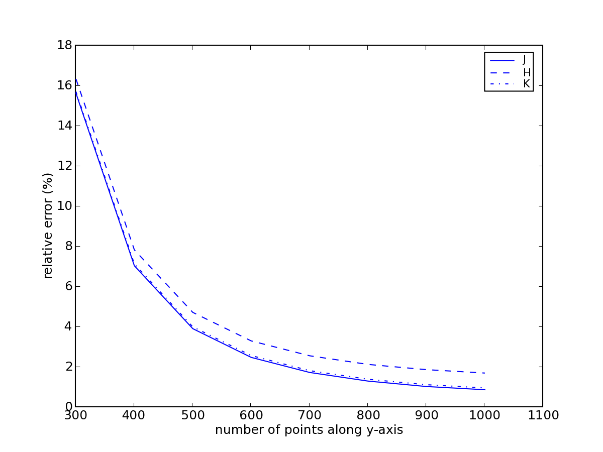
Figure 5: Relative errors between spatial averages of the angular moments $J$, $H$ and $K$ given by the 2D-SOR 2-level iterative process and their analytical values for $\epsilon=0.01$ vs. the number of spatial points of a square 2D grid of extension $\tau^{*}=100$ in each direction.

A stringent test for our 2D code was to consider a point-source located at the center of a non-externally illuminated and homogeneous slab. The central source emits isotropically in space, which in fact corresponds to a line, infinite along $x$, of sources. This idealized model captures most of the difficulties met by the numerical methods to solve the radiative transfer equation: the scattering is not neglected – it can also be dominant –, and the ponctual source will lead to large gradients difficult to handle when dealing with discretization of the slab.

Then we have computed the properties of the radiation field emerging at the top surface of the slab ($z=0$) at one frequency, as described by the usual first three moments $J$, $H$, $K$ of the specific intensity; more precisely, the later were integrated in space, along the top surface of the slab, in order to be compared to the 1D analytical solutions.

To achieve this test, we have chosen the difficult case of a slab of optical thickness $\tau^{*}=100$ in both directions where scattering dominates the absorption adopting the value $\varepsilon=0.01$. This medium is therefore effectively thick because the thermalization depth ${\ell}\approx 1/\sqrt{3\varepsilon}$ is much less than the optical thickness in such as case. We used Carlson’s “Set A” (carlson (1963)) with 10 points per octant to describe the angular dependence of the radiation field and only one frequency-point. The Dirac thermal source term has been modelized by a sharp, normalised 2D-Gaussian function having half-width at half-maximum 0.16 in $\tau$. The grid is logarithmically refined near the center of the slab in order to describe accurately the shape of the 2D-Gaussian: the closest points from the center are at a distance $10^{-4}$ along the axes, in order to accurately describe the gaussian shape whose numerical integral over the space has to be the closest as possible to unity.

The two-level 2D-SOR iterative process was iterated until convergence of $J$, $H$ and $K$ i.e., when the second digit of their relative error did not show any more variation from one iteration to the other. For such a case, 500 iterations are sufficient. In Fig. 5, we demonstrate how these errors behave with the refinement of the spatial quadratures; the absolute values of the reference solutions are given in Appendix, as well as the source functions and values of the specific intensity in the directions corresponding to the angular quadrature chosen here.

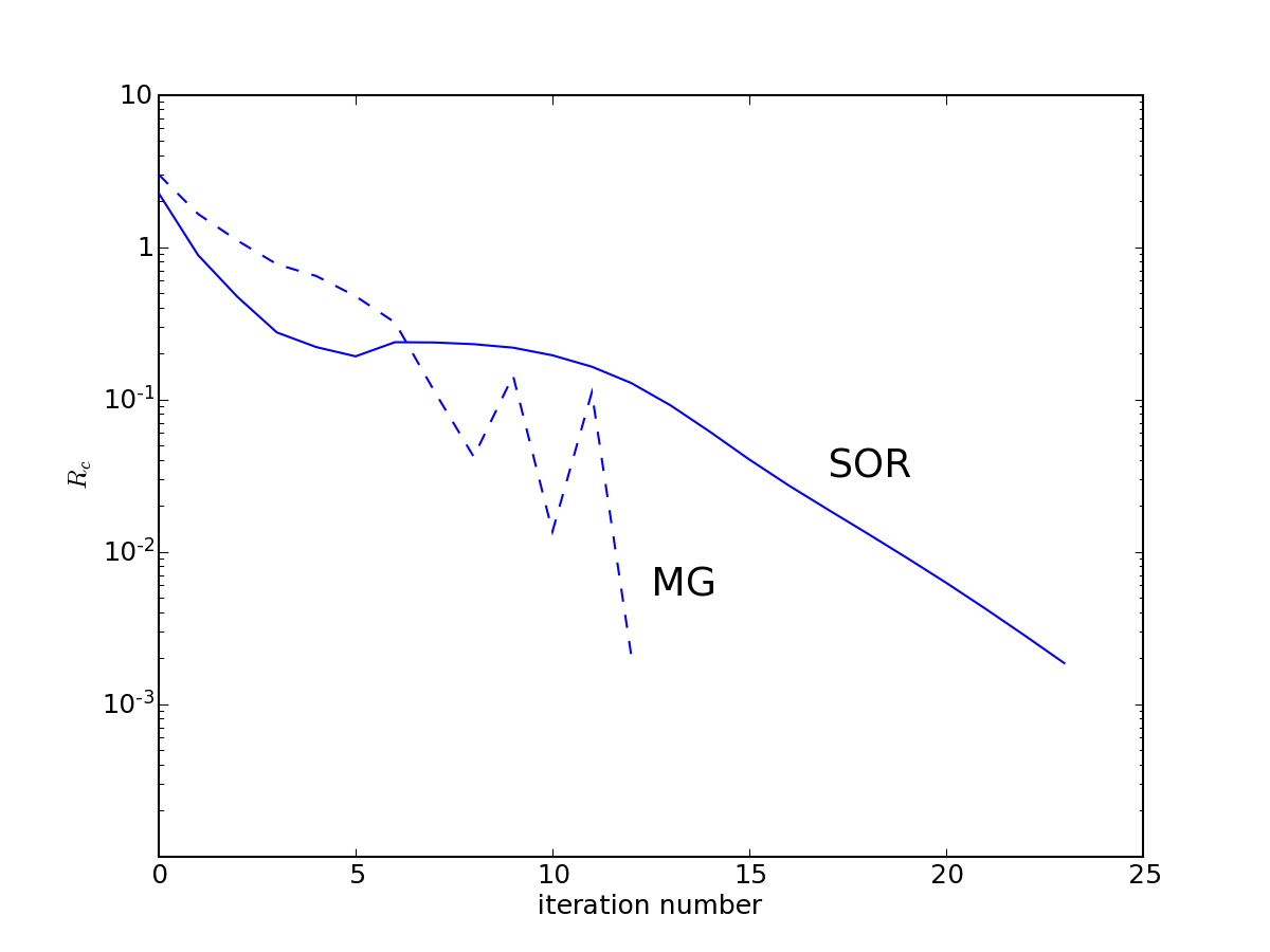
Figure 6: Rates of convergence for the SOR (solid lines) and SOR-MG (dashed lines) 2D multilevel iterative processes. A spatial grid of 163 points per direction with $z_{max}=30\,000$ km and $y_{max}=5\,000$ km; the temperature of the atmosphere is 5 000 K and the gas pressure fixed at $p_{g}\,=\,1\,\mathrm{dyn\,cm^{-2}}$. For benchmark purposes, we adopted the simplified 3-level H i atom model taken from Avrett (avrett (1968)).

The important point to rise here concerning this new test is that (i) acceptable relative errors, say better than 5% are obtained only for very refined grid which (ii) can hardly be handled using a simple Jacobi-like iterative scheme such as ALI. This justify again the adoption of very high rate of convergence methods such as GS/SOR plus MG. Finally, we are conducting more comprehensive tests of this nature which results will be published elsewhere.

5 Illustrative examples and benchmarks

We modeled a 2D freestanding slab irradiated from below on its sides and bottom by a Planck function. The slab is homogeneous and static with a vertical geometrical extension $z_{max}=30\,000$ km; its horizontal extension $y_{max}$ could take the respective values: 100 000, 30 000, 10 000, 5 000 and 1 000 km. Depth points are logarithmically spaced away from the boundary surfaces and the graphical representation we adopted compresses the central region and greatly expand the areas near the boundaries. We have used the “set A” of Carlson (carlson (1963)) with 3 points per octant to describe the angular dependence of the radiation field and constant Doppler profiles. The temperature of the slab was fixed to $T$=5 000 K and the gas pressure $p_{g}=1$  dyn cm^-2. Finally, we adopted the standard benchmark models for multilevel atom problems proposed by Avrett (avrett (1968); see also Paletou & Léger paleg (2007)) considering, in particular, its 3-level H i atomic model.

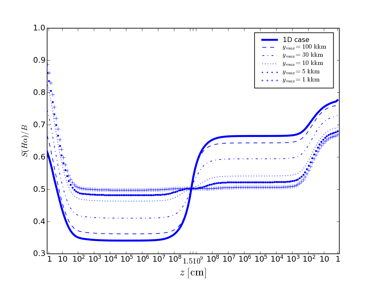
Figure 7: Vertical variations of the H$\alpha$ source function (in units of B) along the symmetry axis of the 2D slab with $z_{max}\,=\,30\,000$ km and different horizontal extensions $y_{max}$ ranging from 1 000 km to $\infty$ (1D); the temperature of the atmosphere is 5 000 K and the gas pressure $p_{g}=1\,\mathrm{dyn\,cm^{-2}}$. The solid line represents S(H$\alpha$)/B variations computed in 1D. Note that abscissae give geometrical positions computed downwards from the top surface up to mid-slab and then, symmetrically, upward from slab bottom.

The respective rates of convergence for the SOR and MG-2D multilevel iterative processes are displayed in Fig. 6 where we have plotted the maximum relative change on the level populations (i.e., the $\infty$-norm) from an iteration to another $R_{c}$. The computation time for the MALI, GS, SOR and MG 2D-multilevel iterative processes are given in Tab. 1 for different grid refinements. We remind that a MG scheme is not only superior in iteration numbers and computing time: it is also important to note that the convergence error $C_{e}$ which is defined by

$$C_{e}=\mathrm{max}\left({{\mid n(itr)-n(\infty)\mid}\over{n(\infty)}}\right)$$ (28)

is smaller than $R_{c}$ for MG whereas for methods such as MALI or SOR a small value of $R_{c}$ does not imply a small value of $C_{e}$, which means that convergence is not necessarily achieved (Fabiani Bendicho et al. fta2 (1997)).

As shown in Fig. 7, where S(H$\alpha$) normalized to the external illumination is plotted as a function of the vertical line-center optical depth, the same variations as in 1D (solid line) are recovered along the vertical axis of symmetry of the 2D model which has the largest horizontal extension (i.e., 10 0000 km). For smaller geometrical slab widths and accordingly horizontal optical thickness, lateral radiative transfer effects take place and progressively affect the excitation within the slab. Note that for the smallest width (i.e., 1 000 km), we properly recover an almost constant value $S/B=0.5$ consistent with optically thin conditions along the horizontal extension of the 2D slab. As first reported by Paletou (fp97 (1997)), we also recover here under which conditions 2D radiative transfer effects on the H$\alpha$ source function vertical variations can be significant; more generally, such effects are a priori expected for any other spectral lines of moderate optical thickness.

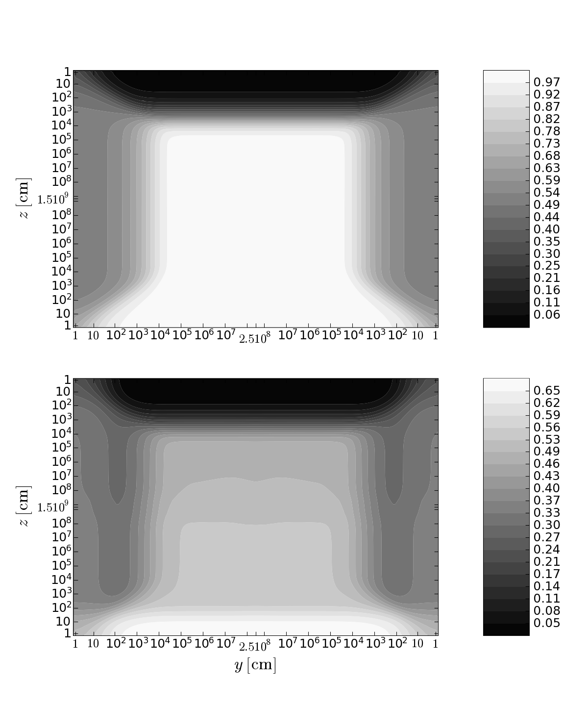
Figure 8: Contour diagram of (top) the second-level populations $n_{2}/n_{2}^{\ast}$ and (bottom) the third-level populations $n_{3}/n_{3}^{\ast}$ in a grid with $y_{max}$=5 kkm, $z_{max}$ =30 kkm, T=5 000 K and $p_{g}=1\,\mathrm{dyn\,cm^{-2}}$. The slab is illuminated from below with a Planck function and $n_{2}^{\ast}$ and $n_{3}^{\ast}$ are LTE values. Horizontal and vertical axes are defined as described in Fig. 7.

Figures 8 are contour plots of the two excited levels of hydrogen normalized to their LTE values obtained for a 30 000 km by 5 000 km slab. They show both departures from LTE together with geometry effects within the slab atmosphere. However, since such data do not exist yet in the litterature while needs for multidimensional radiative modelling tools are more and more obvious, and in order to detail the information content of Fig. 8 about the populations distribution across the 2D slab, we found that Tab. 2 can also be highly valuable for benchmark purposes.

Table 2: Second-level (top) and third-level (bottom) populations for the Avrett (avrett (1968)) H i atomic model in a 2D grid of 163 points per direction with $y_{max}\,=\,5000\,\mathrm{km}$ and $z_{max}\,=\,30000\,\mathrm{km}$ together with 3 angles per octant and 8 frequencies ; the temperature of the atmosphere is 5000 K and the gas pressure $p_{g}\,=\,1\,\mathrm{dyn\,cm^{-2}}$.

					y-position
z-position	$1$	$10$	$10^{2}$	$10^{3}$	$10^{4}$	$10^{5}$	$10^{6}$	$10^{7}$	$10^{8}$	$2.5\times 10^{8}$
$1$	93.6107	52.4326	15.8861	6.29160	5.01322	5.02310	5.02508	5.02511	5.02517	5.02521
$10$	113.845	84.3495	29.7678	11.8603	9.45411	9.47290	9.47663	9.47669	9.47682	9.47690
$10^{2}$	136.951	128.456	86.6607	38.9345	31.1428	31.2092	31.2215	31.2217	31.2222	31.2225
$10^{3}$	145.777	145.248	141.607	121.020	104.541	104.935	104.976	104.977	104.979	104.980
$10^{4}$	148.677	150.732	159.910	188.041	229.865	237.425	237.537	237.539	237.543	237.545
$10^{5}$	149.219	151.755	163.283	199.744	265.198	290.210	291.726	291.727	291.732	291.736
$10^{6}$	149.257	151.825	163.517	200.529	267.018	294.048	296.308	296.366	296.371	296.375
$10^{7}$	149.259	151.829	163.530	200.576	267.127	294.182	296.502	296.640	296.645	296.648
$10^{8}$	149.255	151.823	163.517	200.557	267.101	294.153	296.473	296.611	296.597	296.593
$10^{9}$	149.243	151.801	163.469	200.491	267.010	294.051	296.370	296.509	296.499	296.494
$1.5\times 10^{9}$	149.241	151.798	163.462	200.481	266.996	294.036	296.355	296.495	296.495	296.494
$3\times 10^{9}-10^{9}$	149.239	151.795	163.455	200.471	266.983	294.020	296.339	296.480	296.489	296.493
$3\times 10^{9}-10^{8}$	149.227	151.773	163.408	200.404	266.891	293.918	296.236	296.378	296.392	296.396
$3\times 10^{9}-10^{7}$	149.223	151.767	163.394	200.386	266.866	293.890	296.207	296.348	296.344	296.341
$3\times 10^{9}-10^{6}$	149.223	151.766	163.393	200.384	266.863	293.886	296.204	296.343	296.338	296.334
$3\times 10^{9}-10^{5}$	149.223	151.767	163.396	200.395	266.887	293.944	296.201	296.337	296.331	296.328
$3\times 10^{9}-10^{4}$	149.286	151.886	163.789	201.752	270.398	294.453	296.151	296.261	296.256	296.253
$3\times 10^{9}-10^{3}$	150.529	154.236	171.626	228.713	285.362	295.302	296.043	296.091	296.086	296.083
$3\times 10^{9}-10^{2}$	157.815	168.092	216.220	274.214	292.499	295.409	295.629	295.643	295.639	295.636
$3\times 10^{9}-10$	179.929	210.210	266.745	287.561	293.106	293.988	294.055	294.059	294.057	294.055
$3\times 10^{9}-1$	199.795	241.337	278.860	289.983	292.923	293.390	293.426	293.428	293.427	293.426
					y-position
z-position	$1$	$10$	$10^{2}$	$10^{3}$	$10^{4}$	$10^{5}$	$10^{6}$	$10^{7}$	$10^{8}$	$2.5\times 10^{8}$
$1$	1.86186	1.39630	0.486537	0.153291	0.118500	0.118255	0.118259	0.118240	0.118095	0.118004
$10$	2.04988	1.69002	0.627277	0.207928	0.161807	0.161613	0.161631	0.161604	0.161402	0.161275
$10^{2}$	2.39169	2.20327	1.31802	0.534052	0.422122	0.422372	0.422476	0.422406	0.421855	0.421507
$10^{3}$	2.59030	2.47736	2.04905	1.61663	1.38949	1.39398	1.39445	1.39422	1.39235	1.39117
$10^{4}$	2.65493	2.56695	2.29196	2.50136	3.04375	3.14272	3.14409	3.14357	3.13933	3.13665
$10^{5}$	2.66696	2.58361	2.33664	2.65572	3.50992	3.83926	3.85912	3.85848	3.85327	3.84998
$10^{6}$	2.66789	2.58487	2.33988	2.66628	3.53420	3.89018	3.92008	3.92026	3.91497	3.91163
$10^{7}$	2.66898	2.58607	2.34158	2.66891	3.53832	3.89491	3.92572	3.92885	3.92452	3.92119
$10^{8}$	2.67909	2.59711	2.35631	2.68839	3.56437	3.92360	3.95464	3.95879	3.97321	3.97675
$10^{9}$	2.71539	2.63671	2.40913	2.75824	3.65778	4.02648	4.05820	4.06111	4.07079	4.07557
$1.5\times 10^{9}$	2.72068	2.64248	2.41682	2.76842	3.67139	4.04146	4.07319	4.07500	4.07460	4.07610
$3\times 10^{9}-10^{9}$	2.72615	2.64845	2.42479	2.77894	3.68546	4.05695	4.08873	4.08978	4.08135	4.07652
$3\times 10^{9}-10^{8}$	2.76248	2.68807	2.47763	2.84882	3.77890	4.15986	4.19231	4.19203	4.17766	4.17398
$3\times 10^{9}-10^{7}$	2.77246	2.69897	2.49216	2.86803	3.80459	4.18815	4.22083	4.22152	4.22589	4.22921
$3\times 10^{9}-10^{6}$	2.77348	2.70008	2.49365	2.86999	3.80721	4.19103	4.22384	4.22638	4.23167	4.23501
$3\times 10^{9}-10^{5}$	2.77363	2.70025	2.49389	2.87039	3.80787	4.19223	4.22439	4.22699	4.23228	4.23561
$3\times 10^{9}-10^{4}$	2.77557	2.70281	2.50008	2.89035	3.85874	4.20084	4.22507	4.22730	4.23259	4.23593
$3\times 10^{9}-10^{3}$	2.81121	2.75044	2.62027	3.28700	4.08933	4.23074	4.24134	4.24270	4.24796	4.25128
$3\times 10^{9}-10^{2}$	3.08898	3.10503	3.45736	4.22654	4.48790	4.52946	4.53266	4.53348	4.53832	4.54137
$3\times 10^{9}-10$	3.71314	3.95438	4.74064	5.11335	5.21097	5.22648	5.22770	5.22826	5.23210	5.23452
$3\times 10^{9}-1$	3.99111	4.39634	5.06123	5.33812	5.40867	5.41987	5.42076	5.42127	5.42483	5.42707

6 Conclusions

We have given here details upon the implementation of GS/SOR iterative processes in 2D cartesian geometry, information which was unfortunately still missing in the astrophysical litterature. We also tested, for the first time, such 2D-GS/SOR iterative schemes with a two-level atom model against original analytical results; a more comprehensive study, both in 1D and in 2D, is being conducted and results will be published elsewhere.

Concerning the modelling of illuminated freestanding slabs, even though we used here a quite simple atomic model, we found it to be a necessary stage not only to valid our numerical work but also to take the opportunity to deliver reliable 2D multilevel benchmark results; typical CPU usage numbers were also given, clearly in favour of the combination of SOR plus MG methods for complex radiative modelling.

We anticipate that such numerical techniques and benchmark results will be of interest for the new radiative transfer codes currently in use or under development, not only for applications in solar physics but also for interstellar clouds (see e.g., Juvela & Padoan 2005), circumstellar environments with winds (see e.g., Georgiev et al. 2006) or accretion disks (see e.g., Kor$\check{\rm c}$áková & Kubát 2005) modelling for instance.

Appendix A Test case for a 2D code using 1D reference solutions

We describe a test case for radiative transfer methods in 2D cartesian geometry with stationary media, using 1D reference solutions, which are provided using an analytical method. For this purpose, the ARTY code is the numerical implementation, whose accuracy is better than $10^{-10}$, of exact analytical solutions, based on a mathematical method using the finite Laplace transform (Chevallier & Rutily 2005, Chevallier et al. 2003 and references therein).

Our radiative model describes a 2D medium which can scatter in 3D and is infinite and homogeneous along the $x$-axis ($-\infty\leq x\leq+\infty$, $0\leq y\leq y_{max}$, $0\leq z\leq z_{max}$), thus quantities involved in the radiative transfer equation (RTE) do not depend on $x$. This medium is considered such that there is no incoming flux on its boundaries along the $y$- and $z$-axes. In order to compare this 2D case to 1D solutions from ARTY, we consider here the 2D primary source to be an infinite line along the $x$-axis, located at the center of the slab, emitting isotropically, and the medium homogenous and isotropically scattering; the later is also monochromatic i.e., the RTE does not depend on the frequency (which will not be mentioned hereafter) as this is the case when we describe the continuum or a spectral line with the Milne profile, which is constant over any finite energy range and 0 elsewhere.

We write hereafter the RTE in 2D cartesian geometry, and we show how to compare this 2D solution integrated on the $y$-axis to a 1D solution. Table 3 resumes some values of the 1D solution at the surface $z=0$. The RTE for our 2D model is (cf. Chandrasekhar 1950, Chap. I, Eq. (48) or Pomraning 1973, Eq. (2.60), without derivative over $x$ though)

$$\sin\theta\sin\varphi\frac{\partial I}{\partial y}(y,z,\theta,\varphi)+\cos\theta\frac{\partial I}{\partial z}(y,z,\theta,\varphi)=$$ (29)

$$-\chi[I(y,z,\theta,\varphi)-S(y,z)]\,,$$

where $I$ is the specific intensity of the radiative field at $(y,z)$ and in the direction $(\theta,\varphi)$ of the unit vector ${\bf n}$ whose coordinates along $x$, $y$ and $z$ are $\sin\theta\cos\varphi$, $\sin\theta\sin\varphi$ and $\cos\theta$, respectively. $\chi$ is the constant opacity of the homogeneous medium, and $S$ is the unknown source function which can be written

$$S(y,z)=S^{*}(y,z)+\varpi J(y,z),$$ (30)

where $S^{*}$ describes the primary source function i.e., the direct known radiative field emitted by internal sources, $\varpi=(1-\varepsilon)$ is the constant scattering coefficient of the homogeneous medium for simple scattering processes, usually called albedo, and $J$ is the mean intensity of the radiative field defined as

$$J(y,z)=\frac{1}{4\pi}\int_{0}^{\pi}d\theta\int_{0}^{2\pi}d\varphi\sin\theta\,I(y,z,\theta,\varphi)\,;$$ (31)

the primary source function is

$$S^{*}(y,z)=\frac{L}{\chi}\,\delta(y-{y_{max}\over 2})\delta(z-{z_{max}\over 2})\,,$$ (32)

where $L$ is the luminosity per unit length along the $x$-axis. Dividing by $\chi$ means that the source function is an emissivity divided by the opacity. In order to use 1D solutions as a reference, we must integrate the 2D solutions on $y$ over $[0,y_{max}]$ and on $\varphi$ over $[0,2\pi]$. We thus define new functions as

$$\tilde{I}(z,\theta)=\frac{1}{2\pi}\int_{0}^{y_{max}}dy\int_{0}^{2\pi}d\varphi I(y,z,\theta,\varphi)\,.$$ (33)

Similarly we define $\tilde{S}(z)=\tilde{S}^{*}(z)+\varpi\tilde{J}(z)$, $\tilde{S}^{*}(z)=L/\chi\,\delta(z-z_{max/2})$, $\tilde{J}(z)$ and the two successive moments, the radiative flux $\tilde{H}(z)$ and the radiative pressure $\tilde{K}(z)$ as

$$[\tilde{J},\tilde{H},\tilde{K}](z)=\frac{1}{2}\int_{0}^{\pi}\tilde{I}(z,\theta)[1,\cos\theta,\cos^{2}\theta]\sin\theta d\theta\,.$$ (34)

Integrating over $y$ and $\varphi$, and using the symmetry property valid for $\varphi\in\,[0,\pi]$: $I(y_{max},z,\theta,\varphi)=I(0,z,\theta,\pi+\varphi)$, due to the central primary source, Eq. (29) becomes

$$\frac{\sin\theta}{\pi}\int_{0}^{\pi}\sin\varphi I(y_{max},z,\theta,\varphi)d\varphi+\cos\theta\frac{\partial\tilde{I}}{\partial z}(z,\theta)=$$ (35)

$$-\chi[\tilde{I}(z,\theta)-\tilde{S}(z)]\,,$$

where the integral is nul only for $\theta=0$ or $\pi$; note that this simplification is fictitious as, even for these angles, the source function depends on the mean intensity which depends on the boundaries due to the angular integration. This problem is not classical and we need to let $y_{max}\rightarrow+\infty$ in order to suppress this term i.e., the radiation of the primary source is nul at the infinite and Eq. (35) then reduces to the well-known 1D equation:

$$\mu\frac{\partial I}{\partial z}(z,\mu)=-\chi[I(z,\mu)-S(z)]\,,$$ (36)

where $\mu=\cos\theta$.

Equation (36) is usually expressed in optical depth coordinates $\tau(z)=\int_{z}^{z_{max}}\chi(z^{\prime})dz^{\prime}=\chi(z_{max}-z)$. We do not write the RTE, but the primary source function becomes $S^{*}(\tau)=L\delta(\tau-\tau_{max}/2)$ due to the Dirac transformation $\delta(z)=\chi\delta(\chi z)$. Accordingly our 2D primary source function becomes

$$S^{*}(\tau_{y},\tau_{z})=\chi\,L\,\delta(\tau_{y}-{{\tau_{y_{max}}}\over 2})\delta(\tau_{z}-{{\tau_{z_{max}}}\over 2})\,,$$ (37)

where $\tau_{y}=\chi(y_{max}-y)$ and $\tau_{z}=\chi(z_{max}-z)$. In order to simplify the test of a 2D code with a 1D reference solution, the values $L=1$ and $\chi=1$ should be used.

We give in Table 3 some values of the 1D solution at the surface $z=0$, for the source function, the specific intensity for the directions of the angular grid used in this paper, and its three first moments. When integrating all angles over the azimuthal angle $\varphi$, the 10-points per octant angular quadrature resume to a 4-points per quadrant, i.e. $[J,H,K](z)=\sum_{i=1,4}w_{i}[1,\mu_{i},\mu_{i}^{2}]I(z,\mu_{i})$ for such a case where there is no incoming flux. The four directions $\mu_{i}$ are 0.95118969679, 0.78679579496, 0.57735025883, 0.21821789443 and the integration weights $w_{i}$ are 0.063490696251, 0.091383516788, 0.12676086649, 0.21836490929, respectively. It is interesting to note that, using the reference solutions, the angular quadrature for J, H and K will lead to a relative error equal to 0.8%, 0.3% and 0.4% respectively.

Table 3: Reference solutions from the ARTY code at the surface $z=0$ for our test case with $L=1$, $\chi=1$, $z_{max}=100$ and $\varepsilon=0.01$ (see the text for the values of $\mu_{i}$).

	ARTY results
$S(0)$	$2.710704655\times 10^{-4}$
$J(0)$	$2.738085511\times 10^{-4}$
$H(0)$	$1.600980711\times 10^{-4}$
$K(0)$	$1.130399095\times 10^{-4}$
$I(0,\mu_{1})$	$7.837047273\times 10^{-4}$
$I(0,\mu_{2})$	$6.965481933\times 10^{-4}$
$I(0,\mu_{3})$	$5.880635905\times 10^{-4}$
$I(0,\mu_{4})$	$4.026985767\times 10^{-4}$