Modeling Non-Circular Motions in Disk Galaxies:
Application to NGC 2976

Abstract

We present a new procedure to fit non-axisymmetric flow patterns to 2-D velocity maps of spiral galaxies. We concentrate on flows caused by bar-like or oval distortions to the total potential that may arise either from a non-axially symmetric halo or a bar in the luminous disk. We apply our method to high-quality CO and H$\alpha$ data for the nearby, low-mass spiral NGC 2976 previously obtained by Simon et al., and find that a bar-like model fits the data at least as well as their model with large radial flows. We find supporting evidence for the existence of a bar in the baryonic disk. Our model suggests that the azimuthally averaged central attraction in the inner part of this galaxy is larger than estimated by these authors. It is likely that the disk is also more massive, which will limit the increase to the allowed dark halo density. Allowance for bar-like distortions in other galaxies may either increase or decrease the estimated central attraction.

1. Introduction

One of the first steps toward understanding the formation and evolution of galaxies is a determination of the radial distribution of mass within a representative sample of systems. The rotational balance of stars and gas in the plane of a disk galaxy offers a powerful probe of its mass distribution, and has been widely exploited (Sofue & Rubin, 2001).

When the motions of these tracers are consistent with small departures from circular orbits, the determination of the rotation curve (more precisely, the circular orbital speed profile) is straightforward. However, it has long been known (e.g. Bosma, 1978) that large non-circular motions driven by bar-like or oval distortions, warps, or lopsidedness are common features in galaxy velocity maps, which complicate the determination of the radial mass profile. Yet the observed flow pattern contains a great deal of information about the mass distribution, which we wish to extract from the data.

Since galaxies with closely flat, nearly axisymmetric disks are the exception, it is desirable to be able to estimate a mass profile in the more general cases. A number of techniques, which we review in §2, already exist for this purpose. A procedure for dealing with a warped disk has been successfully developed (e.g. Begeman, 1987) from the first simple tilted ring analyses (e.g. Rogstad et al., 1974), and is now widely used.

Non-axisymmetric distortions to the planar flow can always be described by an harmonic analysis. But the approach pioneered by Franx et al. (1994) for interpreting the resulting coefficients embodies epicycle theory, which is valid only for small departures from circular orbits and may give misleading results if the observed non-circular motions are not small compared with the circular orbital speed. A number of authors (see §2 for references) appear to find significant radial flows with speeds that rival the inferred mean orbital motion. Such flows violate the assumption of small departures from circular motion, are physically not well motivated, and the results are hard to interpret.

We therefore propose here a new technique for fitting a general non-axisymmetric model to the velocity field of a galaxy that allows for large non-circular motions. We develop and apply the method specifically for the case of bar-like or oval distortions, but the procedure is readily generalized for potentials having other azimuthal periodicities.

Our simple kinematic model, which we describe in §3, yields both the mean orbital speed and the amplitudes of the non-circular streaming velocities. It is successful because (1) we invoke a straight bar-like distortion to the potential, (2) we do not need to assume small departures from circular motion, and (3) we fit to the entire velocity field at once.

We apply our method (§4) to the high-quality velocity maps of NGC 2976 that were previously presented by Simon et al. (2003, hereafter SBLB), and find that it suggests a significantly different radial mass profile from that deduced by those authors. We show (§5) the reason for this difference, and argue that a bisymmetric distortion is both a more reasonable physical model, and that it is supported by independent evidence of a bar in this galaxy.

2. Modeling Non-Axisymmetric Flows

2.1. Mathematical preliminaries

The velocity of a star or an element of gas in the plane of the disk of a galaxy generally has two components at each point: tangential, $V_{t}$, and radial, $V_{r}$, relative to any arbitrary center, most conveniently the kinematic center. Without approximation, each component can be expressed as a Fourier series around a circle of radius $r$ in the disk plane:

$$V_{t}(r,\theta)=\bar{V}_{t}(r)+\sum_{m=1}^{\infty}V_{m,t}(r)\cos\left[m\theta+\theta_{m,t}(r)\right]$$ (1)

and

$$V_{r}(r,\theta)=\bar{V}_{r}(r)+\sum_{m=1}^{\infty}V_{m,r}(r)\cos\left[m\theta+\theta_{m,r}(r)\right],$$ (2)

where the coefficients, $V_{m,t}$ and $V_{m,r}$, and phases relative to some convenient axis, $\theta_{m,t}$ and $\theta_{m,r}$, are all functions of $r$. The quantity $\bar{V}_{t}(r)$ is the mean streaming speed of the stars or gas about the center; throughout, we refer to this quantity as the mean orbital speed. The axisymmetric term of the radial motion, $\bar{V}_{r}(r)$, represents a mean inflow or outflow in the disk plane, which gives rise to a “continuity problem” if it is large (Simon et al., 2005).

Galaxies are observed in projection, with inclination $i$, about a major axis, which we choose to define as $\theta=0$ in the above expansions. The line-of-sight velocity is the sum of the projected azimuthal and radial velocities: $V_{\rm obs}=V_{\rm sys}+\sin i(V_{t}\cos\theta+V_{r}\sin\theta)$, where $V_{\rm sys}$ is the systemic velocity of the galaxy. In terms of our Fourier series,

$$V_{\rm obs} = V_{\rm sys}$$ (3)

$$+\sin i\left\{\bar{V}_{t}\cos\theta+\sum_{m=1}^{\infty}V_{m,t}\cos\theta\cos\left[m\theta+\theta_{m,t}\right]\right.$$

$$\left.+\;\bar{V}_{r}\sin\theta+\sum_{m=1}^{\infty}V_{m,r}\sin\theta\cos\left[m\theta+\theta_{m,r}\right]\right\}.$$

Using standard trigonometric relations, this expression can be rewritten as

$${V_{\rm obs}-V_{\rm sys}\over\sin i} = \bar{V}_{t}\cos\theta$$ (4)

$$+\sum_{m=1}^{\infty}{V_{m,t}\over 2}\left\{\cos\left[(m+1)\theta+\theta_{m,t}\right]\right.$$

$$+\left.\cos\left[(m-1)\theta+\theta_{m,t}\right]\right\}+\;\bar{V}_{r}\sin\theta$$

$$+\sum_{m=1}^{\infty}{V_{m,r}\over 2}\left\{\sin\left[(m+1)\theta+\theta_{m,r}\right]\right.$$

$$-\left.\sin\left[(m-1)\theta+\theta_{m,r}\right]\right\}.$$

As is well known (e.g. Canzian, 1993; Schoenmakers et al., 1997; Canzian & Allen, 1997; Fridman et al., 2001), projection therefore causes velocity distortions with intrinsic sectoral harmonic $m$ to give rise to azimuthal variations of orders $m^{\prime}=m\pm 1$ in the corresponding line-of-sight velocities. Thus intrinsic distortions at two different sectoral harmonics give rise to projected velocity features of the same angular periodicity in the data, complicating the determination of all coefficients in the expansion.

2.2. Previous approaches

The principal scientific objective of most spectroscopic observations of disk galaxies is to extract the function $\bar{V}_{t}(r)$, which should be a good approximation to the circular orbital speed if all other coefficients on the right-hand side of eq. 3 are small. With a single slit spectrum along the major axis of the galaxy, one generally sets $V_{\rm obs}=V_{\rm sys}+\bar{V}_{t}(r)\sin i$, implicitly assuming all other terms to be negligible. In this case, the inclination must be determined from other data (e.g. photometry). Differences larger than measurement errors between the approaching and receding sides flag the existence of non-circular motions, but measurements along a single axis do not yield enough information to determine any other coefficient. This and other uncertainties inherent in such deductions are well-rehearsed (van den Bosch & Swaters, 2001; de Blok et al., 2003; Swaters et al., 2003a; Rhee et al., 2004; Spekkens et al., 2005; Hayashi & Navarro, 2007). A two-dimensional velocity map, on the other hand, provides much more information.

Software packages, such as rotcur (Begeman, 1987), allow one to fit the velocity field with a single velocity function $\bar{V}_{t}(r)$ in a set of annuli whose centers, position angles (PAs) and inclinations are allowed, if desired, to vary with radius. This package is ideal for the purpose for which it was designed: to determine the mean orbital speed even when the plane of the disk may be warped. It works well when non-circular motions are small, but yields spurious variations of the parameters when the underlying flow contains non-axisymmetric, especially bisymmetric, distortions.

Barnes & Sellwood (2003) adopted a different approach. They assumed the plane of the disk to be flat, and determined the rotation center, inclination, and PA by fitting a non-parametric circular flow pattern to the entire velocity map. Their method averages over velocity distortions caused by spiral arms, for example, but again may yield spurious projection angles and mean orbital speeds if there is a bar-like or oval distortion to the velocity field over a wide radial range. The rotcurshape program, recently added to the NEMO (Teuben, 1995) package, suffers from the same drawback because it also assumes a flat, axisymmetric disk. Furthermore, it fits multiple parametric components to a velocity field and thus has less flexibility than the Barnes & Sellwood (2003) technique.

Franx et al. (1994) and Schoenmakers et al. (1997) pioneered efforts to measure and interpret the non-axisymmetric coefficients that describe an observed velocity field, and expansions up to order $m^{\prime}\sim 3$ are now routinely carried out (e.g. Wong et al., 2004; Chemin et al., 2006; Simon et al., 2005; Gentile et al., 2007). Their approach assumes departures from circular motion to be small so that the radial and tangential perturbations for any sectoral harmonic can be related through epicycle theory. The technique is therefore appropriate only when all fitted coefficients are small and the mean orbital speed is close to the circular orbital speed that balances the azimuthally averaged central attraction. Wong et al. (2004) present an extensive discussion of this technique and conclude that it is difficult to work backwards from the derived Fourier coefficients to distinguish between different physical models.

Swaters et al. (2003b), SBLB and Gentile et al. (2007) report velocity fields for nearby galaxies that show non-circular motions whose amplitude rivals the mean orbital speed at small $r$. Swaters et al. (2003b) note that their $\bar{V}_{t}(r)$ model fails to reproduce the inner disk kinematics of their target. They correct $\bar{V}_{t}(r)$ for an isotropic velocity dispersion of 8 km/s, but do not attempt to model the isovelocity twists in their H$\alpha$ velocity field. SBLB fit the simplest acceptable model to their data: an axisymmetric flow with just two non-zero coefficients $\bar{V}_{t}(r)$ and $\bar{V}_{r}(r)$. They favor this model over a bar-like distortion partly because the galaxy is not obviously barred, and partly because they find that the $m^{\prime}=3$ components are scarcely larger than the noise (see also §4). The addition of the radial velocity term $\bar{V}_{r}$ allows a more complicated flow pattern to be fitted with an axisymmetric model, which significantly improves the fit to their data. Gentile et al. (2007) do detect a radial $m^{\prime}=3$ component in addition to a strong radial $m^{\prime}=1$ term in the kinematics that they report, which they conclude “are consistent with an inner bar of several hundreds of pc and accretion of material in the outer regions”. Despite finding large non-circular motions, the authors of all three studies nonetheless adopted their derived mean orbital speed as the “rotation curve” of the galaxy, which they assume results from centrifugal balance with the azimuthally averaged mass distribution.

These deductions are suspect, however. As we show below (§5.1), a bisymmetric distortion to the flow pattern may not give rise to a large $m^{\prime}=3$ term in the velocity field, and the smallness of these terms does not establish the absence of a strong bisymmetric distortion. Further, associating the $\bar{V}_{t}$ term with the rotation curve is valid only if all departures from circular motion are small, yet they had found non-circular velocity components almost as large as the mean orbital speed over a significant radial range.

Early work on modeling gas flows in barred galaxies is reviewed in Sellwood & Wilkinson (1993; see their section 6.7). Weiner et al. (2001), Kranz et al. (2003), and Pérez et al. (2004) attempt to build a self-consistent fluid-dynamical model of the non-axisymmetric flow pattern. They estimate the non-axisymmetric part of the mass distribution from photometry and try to match the observed flow to hydrodynamic simulations to determine the amplitude of the non-axisymmetric components of the potential. The objective of this, altogether more ambitious, approach is to determine the separate contributions of the luminous and dark matter to the potential. Here, our objective is more modest: to estimate the mean orbital speed from a velocity map that may possibly be strongly non-axisymmetric. Thus their attempt to separate the baryonic from dark matter contributions seems needlessly laborious for our more limited purpose.

3. A New Approach

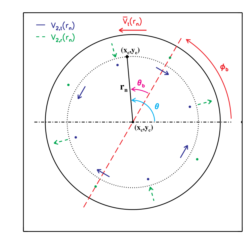
Figure 1.— Parameter definitions and flow pattern in the disk plane for the bisymmetric model (eq. 5). The solid circle represents the largest $r$ included in the model, and the horizontal dash-dotted line is the major axis of the disk defined by the sky plane. The long-dashed line is the major axis of the bisymmetric distortion, at angle $\phi_{b}$ from the major axis. The diamond denotes the location $(x_{e},y_{e})$ of a datapoint $D_{n}$, a distance $r_{n}$ from the kinematic center $(x_{c},y_{c})$ and at PAs $\theta_{b}$ from the bisymmetric distortion axis and $\theta$ from the major axis. The dotted circle shows the circular orbit of radius $r_{n}$ in the disk, and the axisymmetric model component $\bar{V}_{t}(r_{n})$ is in the counter-clockwise direction. The extrema of components $V_{2,t}(r_{n})$ and $V_{2,r}(r_{n})$ are indicated by solid and dashed arrows, respectively, and large dots at the same distance from $(x_{c},y_{c})$ as each set of arrows denote PAs where the corresponding component passes through zero.

3.1. A bar-like distortion

Our objective is to model non-circular motions in a 2-D velocity map. Since we do not wish to assume that non-circular motions are small, we refrain from adopting the epicycle approximation. However, we do make the following assumptions:

• The non-circular motions in the flow stem from a bar-like or oval distortion to an axisymmetric potential. We suppose these motions to be caused by either a non-axially symmetric halo in the dark matter or by a bar in the mass distribution of the baryons.

• A strong bisymmetric distortion to the potential, even one that is exactly described by a $\cos(2\theta)$ angular dependence, can give rise to more complicated motions of the stars and gas (e.g. Sellwood & Wilkinson, 1993). In particular, the flow may contain higher even harmonics. Nevertheless, the $m=2$ terms will always be the largest, and we therefore begin by neglecting higher harmonics.

• We assume the bar-like distortion drives non-circular motions about a fixed axis in the disk plane. In a steady bar-like flow, the perturbed parts of the azimuthal and radial velocities must be exactly out of phase with each other. That is, the azimuthal streaming speed is smallest on the bar major axis and greatest on its minor axis, while radial motions are zero in these directions and peak, with alternating signs, at intermediate angles (Sellwood & Wilkinson, 1993).

• We must assume the disk to be flat, because we require the predicted $V_{\rm obs}$ from eq. 3 to have the same inclination at all $r$. This assumption is appropriate for spiral galaxy velocity fields measured within the optical radius, where warps are rare (e.g. Briggs, 1990), and is therefore well-suited to interpreting kinematics derived from H$\alpha$, CO or stellar spectroscopy. The technique presented here should therefore not be applied to the outer parts of H I velocity fields, which typically extend well into the warp region (e.g. Broeils & Rhee, 1997).

A model based on these assumptions predicts the observed velocity at some general point in the map to be given by eq. 3, with the $m=2$ terms as the only non-axisymmetric terms:

$$V_{\rm model} = V_{\rm sys}\ +\sin{i}\,\,\left[\,\bar{V}_{t}\cos{\theta}-\;V_{2,t}\cos(2\theta_{b})\,\cos{\theta}\right.$$ (5)

$$\left.-\,V_{2,r}\sin(2\theta_{b})\sin{\theta}\,\right]\;.$$

The geometry in the disk plane is sketched in Fig. 1. As above, $\theta$ is the angle in the disk plane relative to the projected major axis, which is marked by the horizontal dash-dotted line. The major axis of the bisymmetric distortion (or bar for short) lies at angle $\phi_{b}$ to the projected major axis; thus angles relative to the bar axis are $\theta_{b}=\theta-\phi_{b}$. We have chosen the phases of the $V_{2,t}$ and $V_{2,r}$ terms such that both are negative at $\theta_{b}=0$ and they vary with angle to the bar as the cosine and sine of $2\theta_{b}$ respectively. Comparing eqs. 3 and 5, we see that $\theta_{2,t}=\pi-2\phi_{b}$ and $\theta_{2,r}=\pi/2-2\phi_{b}$.

The amplitudes of the tangential and radial components of the non-circular flow, $V_{2,t}(r)$ and $V_{2,r}(r)$ respectively, are both functions of radius. While it is possible to relate the separate amplitudes for a given potential, we do not attempt to model the mass distribution that creates the flow and therefore allow them both to vary independently.

Circles in the disk plane project to ellipses on the sky, with ellipticity $\epsilon_{d}$ given by $1-\epsilon_{d}=\cos i$, with a common kinematic center, $(x_{c},y_{c})$. We use primes to denote projected angles onto the sky plane. Thus the projected PA of the disk major axis is $\phi_{d}^{\prime}$, while $\phi_{b}^{\prime}$ is the PA of the bar major axis in the sky plane. These angles are related by

$$\phi_{b}^{\prime}=\phi_{d}^{\prime}+{\rm arctan}(\tan\phi_{b}\cos i)\;.$$ (6)

In addition to the three velocity functions $\bar{V}_{t}(r)$, $V_{2,t}(r)$ and $V_{2,r}(r)$, the model is therefore described by the parameters $(x_{c},\,y_{c},\,V_{\rm sys},\,\epsilon_{d},\,\phi_{d}^{\prime},\,\phi_{b}^{\prime})$. We refer to the model described by eq. 5 as the bisymmetric model.

3.2. Other possible models

Other models for the flow pattern could readily be derived from eq. 3.

In particular, and solely to facilitate comparison with other work, we also fit a purely axisymmetric model with the coefficents of all $m>0$ terms set to zero, but retain the $\bar{V}_{r}$ term. There is no undetermined phase angle for this intrinsically axisymmetric model and the predicted velocity is simply

$$V_{\rm model}=V_{\rm sys}+\sin{i}\;\left[\,\bar{V}_{t}\cos{\theta}+\bar{V}_{r}\sin{\theta}\,\right]\;.$$ (7)

The coefficient $\bar{V}_{r}$ corresponds to pure radial inflow or outflow. We will refer to this as the radial model.

Other, more complicated, models could also be fitted to data by retaining more terms as required, provided that an assumption is made about the radial dependence of the phases of the non-axisymmetric perturbations. The extension of these formulae to include other velocity field harmonics is straightforward, and we have tried doing so in some of our analyses (see §4).

3.3. Discussion

If the non-circular motions measured in some spirals do stem from bar-like or oval distortions, then the bisymmetric model has several advantages over both the radial model and also over epicyclic approaches for characterizing these asymmetries. Since $m^{\prime}=1$ velocity field components can arise from either radial flows or a bisymmetric perturbation to the potential (eq. 4), both the bisymmetric and radial models could produce tolerable fits to the same data. However, the bisymmetric model offers a more direct, unambiguous approach for identifying $m=2$ distortions than does the radial model.

Moreover, interpretations of velocity field harmonics that rely on epicycle theory (Franx et al., 1994; Schoenmakers et al., 1997; Canzian & Allen, 1997) are applicable only in the limit of a weak perturbation to the potential, whereas the components of our bisymmetric model are not restricted to mild distortions. We also note that since the bisymmetric model imposes a fixed $\phi_{b}^{\prime}$ on the non-circular flow pattern, it is not sensitive to $m=2$ perturbations to the potential that are not in phase (such as spiral patterns).

Finally, the bisymmetric technique is much simpler than fluid-dynamical modeling of the velocity field (see §2.2), since it does not require (or yield) a model for the mass distribution.

3.4. Fitting technique

We attempt to fit the above kinematic models to observational data by an extension of the minimization procedure devised by Barnes & Sellwood (2003). In general, we need to determine the systemic velocity $V_{\rm sys}$, kinematic center $(x_{c},y_{c})$, ellipticity $\epsilon_{d}$, and disk PA $\phi_{d}^{\prime}$, as well as $M$ unknown radial functions $V_{m,t}$ and $V_{m,r}$ ($m=0$ and $m>0$ if desired) and the (fixed) PA(s), $\theta_{m}$, of any non-axisymmetric distortions to the flow.

We tabulate each of the $M$ independent velocity profiles at a set of concentric circular rings in the disk plane that project to ellipses on the sky with a common center, $(x_{c},y_{c})$. Once these tabulated values are determined, we can construct a predicted $V_{\rm model}$ at any general point by interpolation. We difference our model from the data, which consist of $N$ line-of sight velocity measurements $\{D_{n}\}$ with uncertainties $\{\sigma_{n}\}$, and adjust the model parameters to determine the minimum $\chi_{\rm r,min}^{2}$ of the standard goodness-of-fit function $\chi_{\rm r}^{2}$ with $\nu$ degrees of freedom:

$$\chi_{\rm r}^{2}=\frac{1}{\nu}\sum_{n=1}^{N}\left(\frac{D_{n}-\sum_{k=1}^{K}w_{k,n}V_{k}}{\sigma_{n}}\right)^{2}\;.$$ (8)

Here, the $K$ elements of $\{V_{k}\}$ are the values of the tabulated velocity profiles in the model and the weights, $w_{k,n}$ describe the interpolation from the tabulated $V_{k}$ to $V_{\rm model}$ (eq. 5 or 7) at the position of the observed value $D_{n}$.

When $\chi_{\rm r}^{2}=\chi_{\rm r,min}^{2}$, the partial gradient of $\chi_{\rm r}^{2}$ with respect to each $V_{j}$, where $j$ labels each of the $V_{k}$ in turn, must satisfy

$${\partial\chi_{\rm r}^{2}\over\partial V_{j}}=-\frac{2}{\nu}\sum_{n=1}^{N}\left(\frac{D_{n}-\sum_{k=1}^{K}w_{k,n}V_{k}}{\sigma_{n}}\right)\frac{w_{j,n}}{\sigma_{n}}=0\;.$$ (9)

Rearranging, we find

$$\sum_{k=1}^{K}\left(\sum_{n=1}^{N}\frac{w_{k,n}}{\sigma_{n}}\,\frac{w_{j,n}}{\sigma_{n}}\right)V_{k}=\sum_{n=1}^{N}\frac{w_{j,n}}{\sigma_{n}^{2}}{D_{n}}\;,$$ (10)

resulting in a linear system of $K$ equations for the $K$ unknowns, $\{V_{k}\}$.

For a given set of attributes $(x_{c},\,y_{c},\,V_{\rm sys},\,\epsilon_{d},\,\phi_{d}^{\prime},\,\theta_{m})$ of the projected disk, we compute $\{V_{k}\}$ by solving the linear system of eq. 10, and use the resulting $\{V_{k}\}$ values in eq. 8 to evaluate $\chi_{\rm r}^{2}$. The best fitting model is found by minimizing eq. 8 over the parameters mentioned above, which necessitates recomputing $\{V_{k}\}$ via eq. 10 at each iteration. Any convenient method may be used to search for the minimum; we use Powell’s direction set method (Press et al., 1992).

Barnes & Sellwood (2003) use this minimization strategy to extract only the mean orbital speed $\bar{V}_{t}(r)$ from H$\alpha$ velocity fields of spirals in the Palunas & Williams (2000) sample. In our more general case, the $M>1$ model profiles are defined by distinct sets of $K^{\prime}_{M}$ rings in the disk plane, and $\{V_{k}\}$ contains all of the velocities from these profiles: $K=\sum_{M}K^{\prime}_{M}$. In other words, adding a velocity profile (defined in $K^{\prime}$ rings) to a model increases the rank of the matrix in eq. 10 by $K^{\prime}$. The radial model has $M=2$, while $M=3$ for the bisymmetric model. Further discussion of $\{V_{k}\}$ and derivations of $\{w_{k,n}\}$ are given in the Appendix.

4. Velocity Field Models of NGC 2976

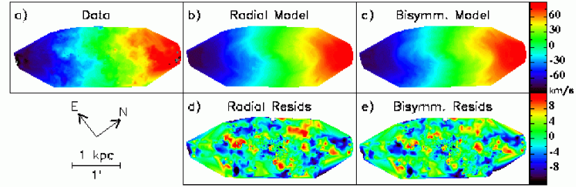
Figure 2.— Kinematic models of the NGC 2976 velocity field. The panels in the top row show (a) the observed velocity field $\{D_{n}\}$ from SBLB, (b) the optimal radial and ($c$) the optimal bisymmetric models. The velocity fields are plotted on the same colorscale, shown in $\rm{km\,s^{-1}}$ to the right of the top row. The panels in the bottom row show residual maps $\{\Delta V_{n}\}=\{D_{n}\ -\sum_{k=1}^{K}w_{k,n}V_{k}\}$ for ($d$) the radial and ($e$) the bisymmetric models, with the colorscale in $\rm{km\,s^{-1}}$ for both shown to the right of that row. The model velocity fields and residuals have been rotated by $-(\phi_{d}^{\prime}\ +\pi/2)$ about $(x_{c},y_{c})$ from Table 1. The data in 2a are rotated by the photometric value $-(-37\arcdeg+\pi/2)$ (intermediate to the two model values) about the photometric center $09^{\mathrm{h}}\,47^{\mathrm{m}}\,15\fs\,3$, $67\arcdeg\,55\arcmin\,00\farcs\,4$ (SBLB). The orientation of $\{D_{n}\}$ (roughly correct for the models as well) and the map scale are at the bottom left. The unusual shape of contoured regions in the maps reflects the locations of the individual pointings used to construct the H$\alpha$ velocity field of NGC 2976 (SBLB).

To illustrate the technique, we fit our bisymmetric model to the observed high-quality velocity field of NGC 2976 reported by SBLB. NGC 2976 is a nearby, low-mass Sc galaxy with $i\sim 60\arcdeg$. We adopt a distance $D=3.56\;$Mpc, estimated from the tip of the red giant branch (Karachentsev et al., 2002), and convert angular scales to linear scales using $1\arcsec=17.3\;$pc.

SBLB present H$\alpha$ and CO velocity fields of NGC 2976, with a spatial resolution of $\sim 5\arcsec$ ($86\,$pc) and spectral resolutions of $13\,\rm{km\,s^{-1}}$ and $2\,\rm{km\,s^{-1}}$, respectively. They find that the velocity field is not well-modeled by disk rotation alone.

They report a detailed analysis of these kinematic data in which the projection geometry of their model rings is determined from optical and near-IR photometry. They conclude that there is no strong evidence for a bisymmetric distortion in this galaxy, since all $m^{\prime}>1$ components of the velocity field are consistent with noise. They find that a combination of rotation and pure radial flows provides an adequate fit. The amplitude of the inferred radial velocity profile rivals that of the rotational component for $r\lesssim 500\,$pc: NGC 2976 thus exhibits some of the largest non-circular motions ever detected in a low-mass, rotationally-supported system. In their later paper, Simon et al. (2005) noted that finding large values of the $\bar{V}_{r}$ term is a strong indication that a model with an axisymmetric radial flow is incorrect. They suggest that the non-circular motions in NGC 2976 stem from a triaxial halo, but their use of epicycle theory relations (Schoenmakers et al., 1997) is inappropriate because $\bar{V}_{r}(r)$ is not always small (see their fig. 9). We also suspect that a bisymmetric distortion is responsible for the observed departures from a circular flow pattern.

The H$\alpha$ and CO velocity fields of NGC 2976 presented in fig. 4 of SBLB were kindly made available to us by J. D. Simon. Following these authors, we analyse the kinematics of the two tracers together, since the data agree within their uncertainties.

We fit the combined velocity field with our bisymmetric model to examine whether the departures from circular motion detected by SBLB stem from an $m=2$ distortion to the potential. In order to demonstrate that our new technique (§3) yields a similar kinematic model to the one obtained by SBLB, we apply our radial model to the same dataset, and compare values of the parameters we obtain as a consistency check on our method. For completeness, we also attempt to fit the data with a suite of other models including $m=0$, $m=1$ and $m=2$ distortions (see below).

The observations presented by SBLB sample the velocity field of NGC 2976 out to $r\sim 130\arcsec$ ($2.2\,$kpc) from its photometric center. We evaluate the velocity profiles in a maximum of $K^{\prime}=26$ rings, separated by 4″ for $r<95\arcsec$ and by up to 10″ farther out. Neither the bisymmetric model nor the radial model yielded reliable constraints on the non-circular components of the velocity field for $r>100\arcsec$. We therefore conclude that the outer part of NGC 2976 is adequately described by a simple circular flow, and fix the amplitudes of all coefficients but $\bar{V}_{t}$ to zero beyond that radius. This reduces the rank of the matrix (eq. 10) by a few.

To check the validity of our planar disk assumption at the largest radii probed by the measurements, we compare the disk parameters derived from fits including different numbers of outer rings. Specifically, each minimization uses the same ring radii, except that the outermost ring included is varied in the range $80\arcsec<r_{\rm max}\ <135\arcsec$ and velocity measurements at radii beyond $r_{\rm max}$ are ignored in the fit. Models with $r_{\rm max}\lesssim 112\arcsec$ return identical disk parameters within the uncertainties, but the optimal values of $x_{c}$, $y_{c}$ and $V_{\rm sys}$ change substantially when rings at larger $r$ are added. We therefore restrict our fits to include only $D_{n}$ with $r_{n}<112\arcsec$ in our final models, as the disk may be warped farther out.

We make an allowance for ISM turbulence by redefining $\{\sigma_{n}\}$ to be the sum in quadrature of the uncertainties in the emission line centroids and a contribution $\Delta_{\rm ISM}=5\,\rm{km\,s^{-1}}$. We find that choosing values of $\Delta_{\rm ISM}$ in the range $3\,\rm{km\,s^{-1}}\lesssim\Delta_{\rm ISM}\lesssim 7\,\rm{km\,s^{-1}}$ and varying the ring locations and sizes by 2–4″ have little impact on our results.

In addition to the bisymmetric and radial models of NGC 2976, we also fitted models including a lopsided ($m=1$) distortion. The optimal $m=1$ model (including velocity profiles $\bar{V}_{t}(r)$, $V_{1,t}(r)$ and $V_{1,r}(r)$; see eq. 3) produced a much less satisfactory fit to the data than either the bisymmetric or the radial model. Adding a radial flow term $\bar{V}_{r}(r)$ yielded optimal parameters identical to those of the radial model, with the $m=1$ components consistent with zero. The insignificance of a lopsided component, which we conclude from these fits, is consistent with our result below that the kinematic and photometric centers of NGC 2976 are coincident within the errors (see also SBLB). We also attempted to fit $m=0$ and $m=2$ distortions to the data simultaneously. Since both cause $m^{\prime}=1$ periodicities in the line-of-sight velocities, however, the resulting model had too much freedom and produced unphysically large variations in all the velocity profiles.

4.1. Uncertainties

The curvature of the $\chi_{\rm r}^{2}$ surface at the minimum implies small formal statistical errors on the best fitting model parameters because of the large numbers of data values. The $\chi_{\rm r,min}^{2}+1.0/\nu$ contour on the $\chi_{\rm r}^{2}$ surface corresponds to variations $\delta V<1\,\rm{km\,s^{-1}}$ on the velocity profile points, which we regard as unrealistically small. We therefore use a bootstrap technique to derive more reasonable estimates of the scatter in the model parameters about their optimal values.

For each model, we generate a bootstrap sample of the data by adding randomly drawn residuals $\Delta V_{n}\ =D_{n}\ -\sum_{k=1}^{K}w_{k,n}V_{k}$ from the distribution at $\chi_{\rm r}^{2}=\chi_{\rm r,min}^{2}$ to the optimal model velocity field. Since $\{\Delta V_{n}\ \}$ is correlated over a characteristic scale corresponding to $J$ adjacent datapoints, fully random selections do not reproduce the quasi-coherent residuals we observe in the data. We therefore select $P=N/J$ values of $\Delta V_{n}$ and add them to the model at $P$ random locations drawn from $\{r_{n},\theta\}$; residuals at the remaining $(1-1/J)N$ in $\{r_{n},\theta\}$ are fixed to the value of the nearest randomly drawn $\Delta V_{n}$. We find that $J=4$ produces bootstrap residual maps with features on scales similar to those in $\{\Delta V_{n}\ \}$ for the models of NGC 2976 in Fig. 2 (see below), but that there is little change in the derived uncertainties for $2\leq J\leq 5$.

For both the bisymmetric and radial models, we therefore construct bootstrap samples of the observed velocity field using $J=4$. We repeat the minimization for each sample, substituting the bootstrap velocities for $\{D_{n}\}$ in eqs. 8 and 10. We carry out this procedure 1000 times, and adopt the standard deviation of each parameter about its mean value from all the realizations as its $1\sigma$ uncertainty in the model of the measured velocities $\{D_{n}\}$.

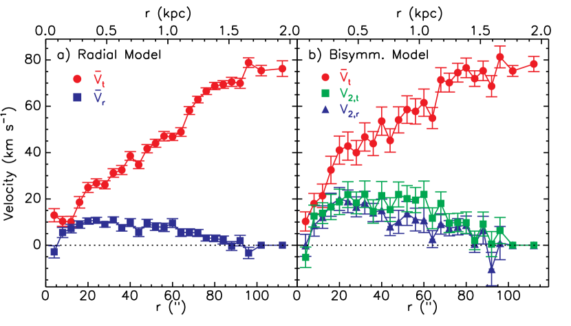
Figure 3.— Fitted velocity components for NGC 2976. (a) The components of the optimal radial model: $\bar{V}_{t}(r)$ is shown by the red circles and $\bar{V}_{r}(r)$ is shown by the blue squares (eq. 7). (b) Velocity components from the optimal bisymmetric model: here $\bar{V}_{t}(r)$ is shown by the red circles, $V_{2,t}(r)$ by the green squares, and $V_{2,r}(r)$ by the blue triangles (eq. 5).

4.2. Results

Our final models of the SBLB H$\alpha$ and CO velocity fields for NGC 2976 are shown in Fig. 2. The minimization results are given in Table 1, and the corresponding velocity profiles are shown in Fig. 3.

The observed velocity field from SBLB is reproduced in Fig. 2a, the best fitting radial and bisymmetric models are in Figs. 2b and 2c, and the residuals $\{\Delta V_{n}\}$ are in Figs. 2d and 2e. Both models reproduce the gross features of the observed velocity field, although the bisymmetric model exhibits a somewhat larger isovelocity contour “twist” along the kinematic minor axis (oriented vertically in Fig. 2) than the radial model. The residual patterns in Figs. 2d and 2e are very similar: $\Delta V_{n}$ is correlated on scales of $15-20\arcsec$ ($250-350\,$pc) in the maps, which may reflect large-scale turbulence. The mean values $\langle|\Delta V_{n}|\rangle$ in Table 1 are slightly lower for the bisymmetric model than for the radial one, as is also suggested by the colors in Figs. 2d and 2e.

The values of $(x_{c},y_{c})$ and $V_{\rm sys}$ in the two models (Table 1) are identical within their uncertainties, while the radial model favors a larger $\epsilon_{d}$ and $\phi_{d}^{\prime}$ than the bisymmetric model at the 2$\sigma$ level. Both sets of kinematic parameters $\left(x_{c},\,y_{c},\,\epsilon_{d},\,\phi_{d}^{\prime}\right)$ are consistent with the photometric values derived by SBLB, corroborating their conclusion that there is little evidence for an offset between them (see also §4). The values of $\chi_{\rm r,min}^{2}$ indicate that both models adequately describe $\{D_{n}\}$, with $\chi^{2}\sim 1$ per degree of freedom for the adopted $\Delta_{\rm ISM}$. Even though the bisymmetric model has fewer $\nu$ than the radial model, the difference between their $\chi_{\rm r,min}^{2}$ is formally significant at the $12\sigma$ level. As with the unrealistically small model uncertainties implied by the $\chi_{\rm r,min}^{2}+1.0/\nu$ contour on the $\chi_{\rm r}^{2}$ surface, however, a literal interpretation this difference in goodness-of-fit is unwise. We thus conclude conservatively that the smaller $\chi_{\rm r,min}^{2}$ and lower $\langle|\Delta V_{n}|\rangle$ of the bisymmetric over the radial model imply only a marginally superior statistical fit to the data.

Figure 4.— Difference $V_{2,t}(r)\ -V_{2,r}(r)$ in the optimal bisymmetric model. The components are plotted separately in Fig. 3b.

Figure 5.— Difference $\Delta\bar{V}_{t}(r)$ between the optimal $\bar{V}_{t}(r)$ from the bisymmetric model and the optimal $\bar{V}_{t}(r)$ from the radial model. The components are plotted separately in Fig. 3.

The best fitting velocity field components from our radial model are shown in Fig. 3a. Despite significant differences between our minimization technique and that of SBLB, our measurements of $\bar{V}_{t}(r)$ and $\bar{V}_{r}(r)$ agree well with their results (the large $\bar{V}_{t}(r)$ for $r\lesssim 10\arcsec$ in our radial model was also found by SBLB in their ringfit velocity field decompositions; see their fig. 7a). We find that $\bar{V}_{r}(r)$ is $\sim 7\,\rm{km\,s^{-1}}$ smaller at $r<30\arcsec$ than the radial velocity amplitudes presented by SBLB. This $\sim 2\sigma$ discrepancy results from our inclusion of a $\Delta_{\rm ISM}$ term in $\{\sigma_{n}\}$ (eqs. 8 – 10), and disappears if we set $\Delta_{\rm ISM}=0$ in our model. Thus our analysis confirms the non-circular motions in NGC 2976 found by these authors.

The bisymmetric model favors a strongly non-axisymmetric flow about an axis inclined $17^{\circ}$ to the projected major axis in the disk plane. The radial variations and uncertainties of all three fitted velocity components are shown in Fig. 3b. The estimated uncertainties on the $\{V_{k}\}$ are larger than those in the radial model (Fig. 3a), consistent with the larger scatter in the profile values from ring to ring. This is likely due to the extra velocity profile relative to the radial model, which gives the bisymmetric model increased flexibility to fit small-scale features. As in the radial model, we find significant non-circular motions, this time in the form of a bisymmetric flow pattern in the disk plane. The overall shape of the non-circular contributions $V_{2,t}(r)$ and $V_{2,r}(r)$ resembles that of $\bar{V}_{r}(r)$ in the radial model: this is reasonable because both models must fit the $m^{\prime}=1$ variations of the velocity field. The difference $V_{2,t}(r)\ -V_{2,r}(r)$ between the bisymmetric components in Fig. 3 is plotted in Fig. 4. There is marginal evidence that $V_{2,t}(r)>V_{2,r}(r)$ for $45\arcsec\lesssim r\lesssim 65\arcsec$, but elsewhere the two components have very similar amplitudes. Linear theory applied to a weak, stationary bar-like distortion produces $V_{2,t}(r)=V_{2,r}(r)$ for a solid-body rotation velocity profile and $V_{2,t}(r)=1.5V_{2,r}(r)$ for a flat one (Sellwood & Wilkinson, 1993). Although linear theory cannot be trusted for strong perturbations, it is somewhat reassuring that it predicts similar $V_{2,t}(r)$ and $V_{2,r}(r)$ for a rising $\bar{V}_{t}(r)$.

The most significant difference between the optimal radial and bisymmetric models is in the shape of $\bar{V}_{t}(r)$. Beyond the region affected by non-circular motions, $r\gtrsim 80\arcsec$, $\bar{V}_{t}(r)$ is identical in the two models, as it must be, but large differences arise where non-circular motions are large. Fig. 5 shows the difference between $\bar{V}_{t}(r)$ from the bisymmetric model and that from the radial model: the former profile rises more steeply than the latter, and its amplitude is larger by $\sim 15\,\rm{km\,s^{-1}}$ for $15\arcsec\lesssim r\lesssim 50\arcsec$. We discuss the reason for these differences in the next section.

Table 1Minimization Results

Model	$\epsilon_{d}$	$\phi_{d}^{\prime}$	$x_{c}$	$y_{c}$	$V_{\rm sys}$	$\phi_{b}^{\prime}$	$\chi_{\rm r,min}^{2}$	$\nu$	$\langle|\Delta V_{n}|\rangle$
		(°)	(″)	(″)	($\rm{km\,s^{-1}}$)	(°)			($\rm{km\,s^{-1}}$)
(1)	(2)	(3)	(4)	(5)	(6)	(7)	(8)	(9)	(10)
radial	$0.568\pm 0.007$	$-36.0\pm 0.6$	$-1.7\pm 0.3$	$0.8\pm 0.4$	$0.3\pm 0.4$	$\cdots$	1.35	1034	3.4
bisymmetric	$0.556\pm 0.007$	$-37.6\pm 0.6$	$-1.9\pm 0.3$	$1.2\pm 0.3$	$0.7\pm 0.4$	$-45\pm 4$	1.20	1009	3.1

Note. — Col. (1): Model. Col. (2): Disk ellipticity. Col. (3): Disk PA, measured North $\rightarrow$ East to the receding side of the disk. Col. (4): Right ascension of disk center, relative to the photometric center $09^{\mathrm{h}}\,47^{\mathrm{m}}\,15\fs\,3$ (SBLB). Col. (5): Declination of disk center, relative to photometric center $67\arcdeg\,55\arcmin\,00\farcs\,4$ (SBLB). Col. (6): Disk systemic velocity, heliocentric optical definition. Col. (7): Bisymmetric distortion PA, measured North $\rightarrow$ East. Col. (8): Minimum value of $\chi_{\rm r}^{2}$ (eq. 8) obtained. Col. (9): Number of degrees of freedom in the minimization. Col. (10): Amplitude of the average (data - model) residual.

5. Discussion

5.1. Mean streaming speed

The large differences in the fitted $\bar{V}_{t}(r)$ for the bisymmetric and radial models over the inner part of NGC 2976 (Fig. 5) demand explanation. Fig. 6 shows sky-plane projections of the angular variations of the separate fitted velocity components at $r=20\arcsec$ for both models.

Fig. 6a shows the projected $\bar{V}_{r}(r)$ of the radial model (dash-dotted line), which shifts the peak in the projected model velocity (solid line) away from the kinematic major axis ($\theta=0$) and reproduces the iso-velocity “twist” in the observed velocity field (Fig. 2). Since the projected $\bar{V}_{r}$ must be zero at $\theta=0$ in this model (see eq. 7), the projected $\bar{V}_{t}(r)$ (dashed line) must equal $V_{\rm model}$ along the kinematic major axis.

Fig. 6b shows the corresponding case for the bisymmetric model where the non-axisymmetric terms allow $V_{\rm model}$ to differ from $\bar{V}_{t}$ along the major axis (eq. 5). The abscissae are marked as $\theta$ along the bottom and as $\theta_{b}$ along the top, which differ only slightly because the best fitting major axis of the bisymmetric distortion in NGC 2976 projects to a PA similar to the kinematic major axis (i.e. $\phi_{b}^{\prime}\sim\phi_{d}^{\prime}$; Table 1). The significant negative contribution of the projected $V_{2,t}(r)$ (dash-dotted line) to $V_{\rm model}$ (solid line) at $\theta=0$ offsets the positive contribution from $\bar{V}_{t}(r)$ (dashed line). The greater amplitude of $\bar{V}_{t}(r)$ in the bisymmetric model of NGC 2976 is therefore due to the large non-circular motions in the inner parts that happen to be negative near the kinematic major axis because the $m=2$ distortion is oriented close to this axis.

Notice also that the $V_{2,t}$ and $V_{2,r}$ components in Fig. 6 show, as they must (§2), both $m^{\prime}=1$ and $m^{\prime}=3$ periodicities, and that both are of similar amplitude (see also Fig. 4). Yet their relative phases ensure that the net effect of the $m^{\prime}=3$ terms on $V_{\rm model}$ cancels almost exactly. A larger $m^{\prime}=3$ signal could arise if the $V_{2,t}$ and $V_{2,r}$ terms have different amplitudes, but their relative phases always ensure at least partial cancellation regardless of the orientation of the projected bar. Thus one should not conclude that a very weak $m^{\prime}=3$ signal in the velocity map implies no significant bisymmetric distortion.

5.2. Centrifugal balance?

It is clear from Table 1 and Fig. 2 that both the bisymmetric and radial models are adequate parameterizations of the observed geometry and kinematics of NGC 2976. But does either model provide insight into its physical structure?

The mean orbital speed, $\bar{V}_{t}(r)$, in the radial model can balance the central attraction of the system only if either the non-circular motions are small, or $\bar{V}_{r}(r)$ actually implies a real radial flow that somehow does not affect orbital balance. The first possibility is not true, as we have confirmed (Figs. 3 and 6) the large non-circular motions found for $r\lesssim 500\,$pc in NGC 2976 by SBLB. If $\bar{V}_{r}(r)$ is attributed to radial flows that do not affect orbital balance, then all of the detected gas in this quiescent system would be displaced on kpc scales in $1-3\,$Gyr; we agree with Simon et al. (2005) that this explanation is not viable. We thus conclude that although the optimal radial model is a reasonable statistical fit to the data and provides strong evidence for non-circular motions, the fitted $\bar{V}_{t}(r)$ cannot be used to determine the mass distribution within NGC 2976.

If the non-circular motions in NGC 2976 are dominated by an $m=2$ perturbation to its potential, then the velocity profiles of the optimal bisymmetric model should better reflect the galaxy’s structure than those of the radial model. While the fitted $\bar{V}_{t}(r)$ rises more steeply in the bisymmetric model, it is merely the average azimuthal speed around a circle, not a precise indicator of circular orbital balance. It should be stressed that circles in the disk plane approximate streamlines only when non-circular motions are small. In a bar-like potential, the gas on the bar major axis will be moving more slowly than average, since it is about to plunge in towards the center, whereas gas at the same galactocentric radius on the bar minor axis will be moving faster than average, since it has arrived there from a larger radius. Under these circumstances, it is not possible to assert that the azimuthal average, $\bar{V}_{t}$, is exactly equal to the circular orbit speed in an equivalent azimuthally averaged mass distribution. The only reliable way to extract the azimuthally averaged central attraction in this case is to find the non-axisymmetric model that yields a fluid dynamical flow pattern to match that observed, and to average afterwards.

Despite these cautionary statements, we suspect that the $\bar{V}_{t}$ curve from the bisymmetric model provides a better estimate, than does that from the radial model, of the azimuthally averaged central attraction in NGC 2976.

5.3. Evidence for a bar

As discussed in §§1 & 3, the elliptical streams of fixed direction and phase in the bisymmetric model could be driven by either a triaxial halo or by a bar in the mass distribution. In either case, the distortion is significant only at $r\lesssim 80\arcsec$ ($1.4\,$kpc; Fig. 3b) in NGC 2976, beyond which the flow appears to be near circular.

The aspherical halo interpretation therefore requires the halo that hosts NGC 2976 to have an asphericity that increases for decreasing $r$. Such an idea was proposed by Hayashi et al. (2007), although other work (Dubinski, 1994; Gnedin et al., 2004; Kazantzidis et al., 2004; Berentzen & Shlosman, 2006; Gustafsson et al., 2006) has indicated a tendency for disk assembly to circularize the potential.

We therefore favor the interpretation that NGC 2976 hosts a bar. Menéndez-Delmestre et al. (2007) have examined the Two Micron All Sky Survey (2MASS; Skrutskie et al., 2006) $J$, $H$ and $K_{s}$ images of NGC 2976 to search for a bar. Their fits to this photometry reveal a radial variation in ellipticity of amplitude $\Delta\epsilon>0.1$ (see also Simon et al., 2005), and their visual inspection of the images reveals a “candidate” bar with ${\rm PA}_{\rm bar}=-43\arcdeg$ and semi-major axis $a=72\pm 5\arcsec$ (see their table 2). Their estimated ${\rm PA}_{\rm bar}$ is fully consistent with our kinematic estimate $\phi_{b}^{\prime}$ (Table 1), and $a$ compares well with the range of $r$ where $V_{2,t}(r)$ and $V_{2,r}(r)$ are non-zero (Fig. 3b). Furthermore, ${\rm PA}_{\rm bar}$ and $\phi_{b}^{\prime}$ are roughly coincident with the apparent major axis of the CO distribution in NGC 2976 (see fig. 4 of SBLB), which suggests that the molecular gas density is larger along this PA than elsewhere in the disk. Thus the 2MASS photometry and CO morphology provide strong supporting evidence that NGC 2976 contains a bar with the properties implied by our bisymmetric model.

5.4. Mass components

Our fits have revealed strong non-circular motions in NGC 2976 that appear to result from forcing by a bar. While $\bar{V}_{t}(r)$ in the bisymmetric model better reflects the azimuthally averaged mass distribution than its counterpart in the radial model, precise statements about the mass budget in NGC 2976 are hampered by our lack of a reliable estimate of the circular orbital speed curve (see §5.2).

The amplitude of the non-circular motions in NGC 2976 implies a relatively large bar mass, which in turn suggests that the disk itself contributes significantly to the central attaction. It is therefore likely that the baryons in NGC 2976 dominate its kinematics well beyond the $r\sim 500\;$pc suggested by the fits of SBLB. Indeed, the steeper rise of $\bar{V}_{t}(r)$ in the bisymmetric model relative to that deduced by SBLB would allow a larger disk mass-to-light ratio (${\cal M}/L$) to be tolerated by the kinematics. This conclusion eases the tension between their dynamical upper bound on the stellar ${\cal M}/L$ and that expected from stellar population synthesis for the observed broadband colors (see §3.1.1 of SBLB, ).

We defer the detailed mass modeling of NGC 2976 required for quantitative estimates of its mass budget to a future paper. Such a study would be assisted by additional kinematic data from extant H I aperture synthesis observations, as well as by decompositions of publicly available infrared photometry from the Spitzer Infrared Nearby Galaxies Survey (Kennicutt et al., 2003).

5.5. Other galaxies

We suggest that our approach could be useful for characterizing the non-circular motions detected in other galaxies, particularly in low-mass systems where the reported non-circular motions are large (Swaters et al., 2003b; Simon et al., 2005; Gentile et al., 2007). It is more direct than interpretations of velocity field Fourier coefficients in the weak perturbation limit, yields physically meaningful kinematic components for systems with bar-like or oval distortions to the potential, and its application is much simpler than that of a full fluid-dynamical model.

We have shown that the velocity field of NGC 2976, when fitted by our bisymmetric model, reveals a steeper inner rise in $\bar{V}_{t}(r)$ than in previous analyses by other methods. Similar findings have been reported by Hayashi & Navarro (2006) and Valenzuela et al. (2007) for other systems. In NGC 2976, the reason for this difference (Fig. 6) is that the $V_{2,t}$ terms happen to partly cancel the $\bar{V}_{t}$ terms, because they have opposite signs on the projected major axis when the bar is oriented close to this direction. It should be clear, however, that the $V_{2,t}$ terms will have the opposite effect if the bar is more nearly aligned with the projected minor axis. Thus even if the non-circular motions detected in other systems result from bars in the potential, it is unlikely that our bisymmetric model will always cause $\bar{V}_{t}(r)$ to rise more steeply than found previously. In any event, it should be clear that when large non-circular flows are present, the mean orbital speed derived from models that use epicycle theory can yield a very misleading estimate of the interior mass needed for centrifugal balance.

6. Conclusions

We have presented a new method for fitting 2-D velocity maps of spiral galaxies that are characterized by non-circular motions. We suppose the potential to contain a bar-like or oval distortion that drives the gas in the disk plane on an elliptical flow pattern of fixed orientation, such as could arise from a triaxial halo or a bar in the mass distribution of the baryons. Our model has important advantages over previous approaches since it is not restricted to small non-circular motions, as is required when epicycle theory is employed, and we do note invoke large radial flows that have no clear physical origin or interpretation.

Our bisymmetric flow model can be fitted to data by a generalization of the technique developed by Barnes & Sellwood (2003). The fit extracts multiple non-parametric velocity profiles from an observed velocity field, and we employ a bootstrap method to estimate uncertainties.

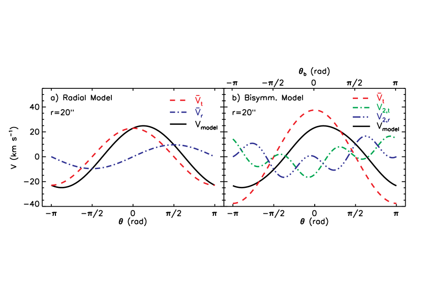
Figure 6.— Projected contributions from different kinematic components at $r=20\arcsec$ ($345\,$pc) in the optimal (a) radial  and (b) bisymmetric  models. In 6a, the dashed line shows the angular dependence of the projected rotational velocity term in the radial model relative to the kinematic major axis ($2^{\mathrm{nd}}$ on the right-hand side (RHS) of eq. 7), and the dash-dotted line shows that of the radial velocity term ($3^{\mathrm{rd}}$ on the RHS of eq. 7). In 6b, the angular dependence of the components in the bisymmetric model are plotted relative to $\phi_{d}^{\prime}$ along the bottom horizontal axis and $\phi_{b}^{\prime}$ along the top horizontal axis. The dashed line shows the rotational velocity term ($2^{\mathrm{nd}}$ on the RHS of eq. 5), and the dash-dotted and dash-dot-dotted lines show the tangential and radial bisymmetric terms, respectively ($3^{\mathrm{rd}}$ and $4^{\mathrm{th}}$ on the RHS of eq. 5). The solid lines in both panels shows the net projected model velocity relative to $V_{\rm sys}$.

As an example, we have applied our technique to the H$\alpha$ and CO kinematics of NGC 2976 presented by SBLB. We show that the bisymmetric model fits the data at least as well as the ringfit procedure implemented by these authors that invokes large radial velocities, which we are also able to reproduce by our methods. Both the bisymmetric and radial models reveal large non-circular motions in NGC 2976, but the derived mean orbital speed profiles $\bar{V}_{t}(r)$ differ markedly between the two cases. We explain the reason for this large difference in §5.

When disks are observed in projection, kinematic distortions with intrinsic sectoral harmonic $m$ cause azimuthal variations of orders $m^{\prime}=m\pm 1$ in line-of-sight velocity maps. Our analysis of NGC 2976 clearly demonstrates that $m^{\prime}=1$ distortions to its velocity field can be fitted by a bisymmetric distortion to the potential, which we regard as more physically reasonable than radial flows. We show in Fig. 6 that $m^{\prime}=3$ distortions should be small in the bisymmetric model; this is because the $m^{\prime}=3$ variations in the radial and tangential components project out of phase. They will cancel exactly only when of equal amplitude, which should be approximately true in the rising part of $\bar{V}_{t}(r)$.

We suggest that NGC 2976 hosts a strong bar oriented at $\sim 17^{\circ}$ to the projected major axis. Our interpretation is supported by its CO morphology (SBLB) and more strongly by the results of Menéndez-Delmestre et al. (2007), who analyzed the 2MASS photometry of NGC 2976 and found a bar whose size and orientation are similar to those required by our bisymmetric model.

We find that the mean orbital speed in NGC 2976 rises more steeply than indicated by previous studies (SBLB; Simon et al. 2005). While $\bar{V}_{t}(r)$ in our bisymmetric model is not an exact measure of the circular orbital speed in the equivalent axially symmetrized galaxy, we regard it as a better approximation to this quantity. Since the strongly non-circular flow pattern implies a massive bar, which in turn suggests a massive disk, we expect a larger baryonic mass than was estimated by SBLB. It is likely, therefore, that most of the increased central attraction required by our more steeply rising $\bar{V}_{t}(r)$ will not reflect a corresponding increase in the density of the inner dark matter halo, but will rather ease the tension between maximum disk fits to its kinematics and ${\cal M}/L$ predictions from broadband photometry (SBLB). Indeed, since non-circular motions are detected throughout the region $r\lesssim 80\arcsec$ ($1.4\,$kpc), it seems likely that the luminous matter in NGC 2976 is an important contributor to the central attraction at least as far out as this radius. Detailed mass models of this system are forthcoming.

Application of our method to other galaxies will not always result in a steeper inner rise in the mean orbital speed. We find this behavior in NGC 2976 only because the bar is oriented near to the projected major axis. Neglect of non-cirular motions, or application of a radial flow model, when the bar is oriented close to the projected minor axis will lead to an erroneously steep rise in the apparent inferred mean orbital speed, which will rise less steeply when our model is applied.

Appendix A Kinematic Model Weights

We use the same notation and parameter definitions as in §3 and Fig. 1. Let $(x_{n},y_{n})$ be the location, in the sky plane, of the $n$th measured velocity $D_{n}$, where $\hat{x}$ points West and $\hat{y}$ points North. Let $\phi_{d}^{\prime}$ be the PA of the projected major axis. The coordinates $(x_{e},y_{e})$ centered on $(x_{c},y_{c})$ and aligned with the projection are:

$$x_{e} = -(x_{n}-x_{c})\sin{\phi_{d}^{\prime}}+(y_{n}-y_{c})\cos{\phi_{d}^{\prime}}$$

$$y_{e} = -(x_{n}-x_{c})\cos{\phi_{d}^{\prime}}-(y_{n}-y_{c})\sin{\phi_{d}^{\prime}}.$$ (A1)

The radius $r_{n}$ of the circle in the disk plane that passes through the projected position of $(x_{n},y_{n})$ is given by

$$r_{n}^{2}=x_{e}^{2}+\left(\frac{y_{e}}{1-\epsilon_{d}}\right)^{2}\;,$$ (A2)

where $\epsilon_{d}$ is the ellipticity of the circle caused by projection; i.e. $\epsilon_{d}=1-\cos i$ for the thin gas layer considered here, where $i$ is the galaxy inclination. Thus the PA, $\theta$, of the measurement at $(x_{n},y_{n})$ relative to the disk major axis (see Fig. 1) satisfies

$$\cos{\theta}=\frac{x_{e}}{r_{n}}\;,$$ (A3)

$$\sin{\theta}=\frac{y_{e}}{(1-\epsilon_{d})r_{n}}\;.$$ (A4)

We tabulate each of the non-parametric velocity profiles at a set of radii in the disk plane that project to ellipses on the sky with semi-major axes $\{{a_{k^{\prime}m}}\}$. The elements of $\{V_{k}\}$ include all $K=\sum_{M}K^{\prime}_{M}$ values from the $M$ velocity profiles combined. In principle, we could employ different numbers of rings $K^{\prime}_{M}$, with differing choices for the $\{a_{k^{\prime}m}\}$ for each velocity profile, but here we evaluate all profiles at the same $K^{\prime}$ locations $\{a_{k^{\prime}}\}$. There are $K^{\prime}_{1}$ radii that define $\bar{V}_{t}(r)$ in our models (eqs. 5 and 7), but we restrict the number of rings describing the non-circular components to $K^{\prime\prime}<K^{\prime}$ when the latter are not well-constrained in the outer disk. In addition, we include the systemic velocity $V_{\rm sys}$ as the $K^{\mathrm{th}}$ element of $\{V_{k}\}$, with $w_{K,n}=1$ for all $D_{n}$.

We use linear interpolation between the two rings that straddle each data point. If $a_{k}\leq r_{n}<a_{k+1}$, the values of $\{w_{k,n}\}$ for that velocity profile and that $D_{n}$ are

$$w_{k,n} = \left(1-\frac{r_{n}-a_{k}}{\delta a_{k}}\right)W_{n}$$

$$w_{k+1,n} = \left(\frac{r_{n}-a_{k}}{\delta a_{k}}\right)W_{n}$$

$$w_{k^{\prime},n} = 0\qquad\mathrm{for}\,\,\,\,k^{\prime}\neq k,\,k+1\,\,\,,$$ (A5)

where $\delta a_{k}=a_{k+1}-a_{k}$ is the ring spacing. The parameter $W_{n}$ in eq. A5 is the combination of trigonometric factors in the dependence of $\{w_{k,n}\}$ on the projection geometry. It is clear from eqs. 5 and 7 that we require a different $W_{n}$ for each $D_{n}$ and for each velocity profile in the bisymmetric and radial models.

For the $\bar{V}_{t}$ component in both models, we have

$$W_{n}=\sin{i}\cos{\theta}\;,$$ (A6)

where $\cos{\theta}$ is given in eq. A3; for the $V_{2,t}$ component in the bisymmetric model

$$W_{n}=\sin{i}\cos(2\theta_{b})\cos{\theta}\;,$$ (A7)

and for the $V_{2,r}$ component

$$W_{n}=\sin{i}\sin(2\theta_{b})\sin{\theta}\;.$$ (A8)

Finally, $W_{n}$ for the $\bar{V}_{r}$ component in the radial model is

$$W_{n}=\sin{i}\sin{\theta}\;.$$ (A9)

References

- Barnes & Sellwood (2003) Barnes, E. I., & Sellwood, J. A. 2003, AJ, 125, 1164
- Begeman (1987) Begeman, K. G. 1987, Ph.D. Thesis, Univ. of Groningen
- Berentzen & Shlosman (2006) Berentzen, I., & Shlosman, I. 2006, ApJ, 648, 807
- Bosma (1978) Bosma, A. 1978, Ph.D. Thesis, Groningen Univ.
- Briggs (1990) Briggs, F. H. 1990, ApJ, 352, 15
- Broeils & Rhee (1997) Broeils, A. H., & Rhee, M.-H. 1997, A&A, 324, 877
- Canzian (1993) Canzian, B. 1993, ApJ, 414, 487
- Canzian & Allen (1997) Canzian, B., & Allen, R. J. 1997, ApJ, 479, 723
- Chemin et al. (2006) Chemin, L., et al. 2006, MNRAS, 366, 812
- de Blok et al. (2003) de Blok, W. J. G., Bosma, A., & McGaugh, S. 2003, MNRAS, 340, 657
- Dubinski (1994) Dubinski, J. 1994, ApJ, 431, 617
- Franx et al. (1994) Franx, M., van Gorkom, J. H., & de Zeeuw, T. 1994, ApJ, 436, 642
- Fridman et al. (2001) Fridman, A. M., Khoruzhii, O. V., Lyakhovich, V. V., Sil’chenko, O. K., Zasov, A. V., Afanasiev, V. L., Dodonov, S. N., Boulesteix, J. A&A, 371, 538
- Gentile et al. (2007) Gentile, G., Salucci, P., Klein, U., & Granato, G. L. 2006, MNRAS, 375, 199
- Gnedin et al. (2004) Gnedin, O. Y., Kravtsov, A. V., Klypin, A. A., & Nagai, D. 2004, ApJ, 616, 16
- Gustafsson et al. (2006) Gustafsson, M., Fairbairn, M., & Sommer-Larsen, J. 2006, Phys. Rev. D, 74, 123522
- Hayashi & Navarro (2007) Hayashi, E., & Navarro, J. F. 2006, MNRAS, 373, 1117
- Hayashi et al. (2007) Hayashi, E., Navarro, J. F., & Springel, V. 2006, MNRAS, 377, 50
- Karachentsev et al. (2002) Karachentsev, I. D., et al. 2002, A&A, 383, 125
- Kazantzidis et al. (2004) Kazantzidis, S., Kravtsov, A. V., Zentner, A. R., Allgood, B., Nagai, D., & Moore, B. 2004, ApJ, 611, L73
- Kranz et al. (2003) Kranz, T., Slyz, A., & Rix, H.-W. 2003, ApJ, 586, 143
- Kennicutt et al. (2003) Kennicutt, R. C., Jr., et al. 2003, PASP, 115, 928
- Menéndez-Delmestre et al. (2007) Menéndez-Delmestre, K., Sheth, K., Schinnerer, E., Jarrett, T. H., & Scoville, N. Z. 2007, ApJ, 657, 790
- Palunas & Williams (2000) Palunas, P., & Williams, T. B. 2000, AJ, 120, 2884
- Pérez et al. (2004) Pérez, I., Fux, R., & Freeman, K. 2004, A&A, 424, 799
- Press et al. (1992) Press, W. H., Flannery, B. P., Teukolsky, S. A., & Vetterling, T. A. 1992, Numerical Recipes (Cambridge: Cambridge Univ. Press)
- Rhee et al. (2004) Rhee, G., Valenzuela, O., Klypin, A., Holtzman, J., & Moorthy, B. 2004, ApJ, 617, 1059
- Rogstad et al. (1974) Rogstad, D. H., Lockart, I. A., & Wright, M. C. H. 1974, ApJ, 193, 309
- Schoenmakers et al. (1997) Schoenmakers, R. H. M., Franx, M., & de Zeeuw, P. T. 1997, MNRAS, 292, 349
- Sellwood & Wilkinson (1993) Sellwood, J. A., & Wilkinson, A. 1993, Reports of Progress in Physics, 56, 173
- Simon et al. (2003) Simon, J. D., Bolatto, A. D., Leroy, A., & Blitz, L. 2003, ApJ, 596, 957 (SBLB)
- Simon et al. (2005) Simon, J. D., Bolatto, A. D., Leroy, A., Blitz, L., & Gates, E. L. 2005, ApJ, 621, 757
- Skrutskie et al. (2006) Skrutskie, M. F., et al. 2006, AJ, 131, 1163
- Sofue & Rubin (2001) Sofue, Y., & Rubin, V. 2001, ARA&A, 39, 137
- Spekkens et al. (2005) Spekkens, K., Giovanelli, R., & Haynes, M. P. 2005, AJ, 129, 2119
- Swaters et al. (2003b) Swaters, R. A., Verheijen, M. A. W., Bershady, M. A., & Andersen, D. R. 2003, ApJ, 587, L19
- Swaters et al. (2003a) Swaters, R. A., Madore, B. F., van den Bosch, F. C., & Balcells, M. 2003, ApJ, 583, 732
- Teuben (1995) Teuben, P. 1995, ASP Conf. Ser. 77: Astronomical Data Analysis Software and Systems IV, 77, 398
- Valenzuela et al. (2007) Valenzuela, O., Rhee, G., Klypin, A., Governato, F., Stinson, G., Quinn, T., & Wadsley, J. 2007, ApJ, 657, 773
- van den Bosch & Swaters (2001) van den Bosch, F. C., & Swaters, R. A. 2001, MNRAS, 325, 1017
- Weiner et al. (2001) Weiner, B. J., Sellwood, J. A., & Williams, T. B. 2001, ApJ, 546, 931
- Wong et al. (2004) Wong, T., Blitz, L., & Bosma, A. 2004, ApJ, 605, 183