SPECTRAL PROPERTIES FROM ${\rm Ly}{\alpha}$ TO ${\rm H}{\alpha}$ 
FOR AN ESSENTIALLY COMPLETE SAMPLE OF QUASARS I: Data

Abstract

We have obtained quasi-simultaneous ultraviolet-optical spectra for 22 out of 23 quasars in the complete PG-X-ray sample with redshift, z $<0.4$, and M${}_{\rm B}<-23$. The spectra cover rest-frame wavelengths from at least ${\rm Ly}{\alpha}$ to ${\rm H}{\alpha}$. Here we provide a detailed description of the data, including careful spectrophotometry and redshift determination. We also present direct measurements of the continua, strong emission lines and features, including ${\rm Ly}{\alpha}$, Si iv+O iv] $\lambda$1400, C iv, C iii], Si iii], Mg ii, ${\rm H}{\beta}$, [O iii], He i $\lambda$5876+Na i $\lambda\lambda$5890,5896, ${\rm H}{\alpha}$, and blended iron emission in the UV and optical. The widths, asymmetries and velocity shifts of profiles of strong emission lines show that C iv and ${\rm Ly}{\alpha}$ are very different from ${\rm H}{\beta}$ and ${\rm H}{\alpha}$. This suggests that the motion of the broad line region is related to the ionization structure, but the data appears not agree with the radially stratified ionization structure supported by reverberation mapping studies, and therefore suggest that outflows contribute additional velocity components to the broad emission line profiles.

1 INTRODUCTION

QSOs appear to be signposts to galaxy evolution. Supermassive black holes have been discovered in nearby galaxies, with masses $M_{\rm BH}$ tightly related to host-galaxy bulge properties, e.g., the stellar velocity dispersion (Tremaine et al., 2002, and references therein) and luminosity (Marconi & Hunt, 2003, & references therein). There is little doubt that these are the black-hole relics of the luminous QSOs in their heyday at redshifts $z\approx 2$–3. It is likely that QSOs and their hosts evolve symbiotically. The host supplies fuel to an accreting black hole, perhaps through merger-driven star formation. To enable fuel to feed the disk, the central system must lose angular momentum, with this loss possibly via winds seen in emission (Leighly & Moore, 2004; Leighly, 2004) and absorption or as more collimated jets.

Fundamental parameters of the central engine are bolometric luminosity $L_{Bol}$ ($\propto$ $\dot{M}$) representing the fueling rate and efficiency, black hole mass $M_{\rm BH}$, and Eddington accretion ratio $L_{Bol}/L_{Edd}$, also angular momentum of the black hole. Observationally, there are many trends and potential clues to the nature of this central engine, from the radio to X-ray, from spectral energy distributions, and lines in emission and absorption. While any understanding is incomplete without including the entire observational domain, here we are concerned with QSOs’ UV-optical continua and emission lines. Much of the diversity in QSO UV-optical spectra can be accounted for by two strong empirical relationships apparently related to fundamental parameters of the central engine: Boroson & Green’s eigenvector 1 relationship (BGEV1, Boroson & Green, 1992, hereafter BG92) and the Baldwin Effect (BE).

The original BE shows an anticorrelation between C iv equivalent width (EW) and UV luminosity (Baldwin, 1977). It was later confirmed that many other UV lines show similar relationships (e.g., Kinney et al., 1990; Laor et al., 1994a, 1995; Wills et al., 1999a) which may depend on the ionization potentials of the corresponding ions (Espey & Andreadis, 1999; Green et al., 2001; Kuraszkiewicz et al., 2002; Croom et al., 2002; Dietrich et al., 2002).

BGEV1 is the first (i.e., most significant) eigenvector discovered from a principal component analysis (PCA) of measured quasar emission properties in the ${\rm H}{\beta}$ region (Boroson & Green, 1992). PCA is a multivariate analysis. It defines new eigenvectors, which are linear combinations of input observables and can reveal important relationships of the observables (see Francis & Wills, 1999, for a detailed description). The original Eigenvector 1 relationship found in the ${\rm H}{\beta}$ region is characterized by the strong anticorrelation between [O iii] and Fe ii strengths, and involves other parameters such as ${\rm H}{\beta}$ FWHM and asymmetry (BG92). BG92 suggested this set of relationships was driven by $L_{Bol}/L_{Edd}$. This was further supported by Laor et al. (1994b, 1997a), additionally finding that narrower ${\rm H}{\beta}$, stronger Fe ii, and weaker [O iii] corresponds to steeper soft X-ray spectra.

In an attempt to understand the above relationships, we obtained quasi-simultaneous UV-optical spectra over the entire ${\rm Ly}{\alpha}$–${\rm H}{\alpha}$ range for 22 of the 23 quasars of the Bright Quasar Survey investigated for soft X-ray properties by Laor et al. (1994b, 1997a) (see §2.2). We extended the spectra to the UV and showed, by principal components analysis, the important extension of BGEV1 into the ultraviolet, as well as demonstrating that BG’s luminosity-dependent eigenvector was actually directly related to the Baldwin Effect in the UV (Wills et al., 1999b, c; Francis & Wills, 1999; Wills et al., 1999a, 2000). Shang et al. (2003) carried out a spectral principal components analysis (SPCA) of the same sample. SPCA decomposes the input spectra into fewer significant orthogonal (i.e., independent) principal eigenvectors (or eigenspectra), which reveal important relationships among the spectral features (see Francis et al., 1992; Francis & Wills, 1999). The first principal eigenvector in Shang et al. (2003) represents the BE, and nicely links the equivalent widths of many ultraviolet lines with the optical, including the broad He ii $\lambda$4686 line, whose inverse luminosity dependence was directly demonstrated by Boroson & Green (1992) and Boroson (2002). The second principal component was the result of differences in continuum shape. The third principal component extends BGEV1 to the UV, showing correlations among broad line widths, and strengths. These first three principal components accounted for 78% of intrinsic variance among spectra in the sample, demonstrating that these relationships are so clear and obvious, that only a small sample is needed to reveal them.

The technique of SPCA has the distinct advantage that correlations among emission and absorption lines can be seen independently of having to define a continuum for these blended features, or to measure specific line-profile parameters. Results over the entire wavelength range are immediately visible, revealing correlations that may not otherwise have been sought. However, disadvantages of SPCA are that the only directly interpretable relationships are those that can be represented by linear relations among the many flux bins along the spectrum. Non-linear dependences caused by differences in line widths, asymmetries, and shifts, or non-linear relationships among emission line EWs, as would be present in the BE over a sufficiently wide luminosity range, are more easily investigated by direct line measurements.

Thus we must also investigate relationships among directly measured spectral parameters. Here we provide a detailed description of the data and direct measurements of the continua, and all strong emission lines and features. We also present the distribution and relationships of emission line profile properties, including line width, velocity shift, and asymmetry. We will expand our previous analyses with new measurements and more parameters in a subsequent paper. For our cosmology, we choose zero cosmological constant, $H_{0}=75\,{\rm km~{}s}^{-1}\mbox{Mpc}^{-1}$, and $q_{0}=0.5$.

2 SAMPLE AND DATA

2.1 Sample

We use the same complete sample of 23 QSOs selected by Laor et al. (1994b, 1997a) from the Bright Quasar Survey (BQS; Schmidt & Green, 1983). Laor et al. aimed to test models of the optical to X-ray continuum, and photoionization of the regions producing optical emission lines. They therefore optimized the sample for observations of the rest-frame soft X-rays by choosing a complete sample of bright, low redshift ($z\leq 0.4$) QSOs, with Galactic H i column density $N_{\rm HI}<1.9\times 10^{20}{\rm cm}^{-2}$ to minimize soft-X-ray absorption. Note that the incompleteness of the BQS discussed by Jester et al. (2005) does not bias our low-redshift ($z<0.4$) sample, since the color-related bias only affect objects with redshifts of $0.5<z<1.0$. For our UV-optical observations, the low redshift allows investigation of UV spectra with much reduced contamination from intergalactic absorption lines and the low $N_{\rm HI}$ ensures small corrections for Galactic reddening. The QSOs in our sample are listed in Table 1 along with their redshifts, magnitudes, soft X-ray spectral index $\alpha_{\rm X}$, and radio loudness.

2.2 Observations

Figure 1 presents the wavelength coverage for all spectral observations and the colors distinguish different observing runs. Table 2 lists observing dates for each spectrum.

UV spectra of all 22 objects were obtained in ACCUM mode with Hubble Space Telescope (HST) Faint Object Spectrograph (FOS, Keyes et al., 1995), covering wavelengths from below ${\rm Ly}{\alpha}$ to beyond the atmospheric cutoff near 3200 Å in the observed frame. Instrumental resolution for all the UV data is equivalent to $\sim$230 ${\rm km~{}s}^{-1}$ (FWHM).

Optical data were obtained at McDonald Observatory except for some HST FOS data and a little early archival data (see Appendix A).

On the Harlan J. Smith 2.7m reflector, the Large Cassegrain Spectrograph (LCS) was used with a Craf-Cassini detector (CC1, a thick chip with excellent cosmetic quality). Some observations of 1996 April and May used Electronic Spectrograph 2 (ES2) on the Otto Struve 2.1m reflector (F1) with CC1 and a thinned Texas Instruments detector (TI1), respectively.

Optical observations were made generally at airmasses less than 1.3, using long slits – both narrow and wide. The narrow slit (1″– 2″) was used for best spectral resolution, and to reduce scattered, background sky, and host-galaxy light. Wide slits (8″ on LCS, 9.1″ on ES2) were used for absolute flux-density calibration (§2.3.2). The wavelength resolution with the narrow LCS slit and ES2 slit was typically $\sim 7.5$Å FWHM, but 6.7Å for ES2 in 1996 May, equivalent to 450 to $\sim$ 300 ${\rm km~{}s}^{-1}$(FWHM) in the ${\rm H}{\beta}$ to ${\rm H}{\alpha}$ region. The slit orientation was east-west, except in one case where the spectrograph was rotated to avoid a contaminating star. Flux density standard stars were observed several times each night, chosen to be close in time and airmass to the QSOs. These standards were chosen from the HST list (Bohlin, 1996, 2000) and their flux calibration files were obtained from HST CALSPEC (ftp://ftp.stsci.edu/cdbs/cdbs2/calspec/, February, 1996 update), to ensure consistent calibration between UV and optical data. Preference was given to the available standards of highest priority (see Bohlin, 1996, 2000).

To reduce the uncertainty caused by QSO intrinsic variability, we attempted to get quasi-simultaneous optical observations. These were usually obtained within a month of the new HST observations for 11 objects and 2–10 months for another 5 objects. Quasi-simultaneous observations were not possible for HST archival data. In table 2, time gaps between observations of each object are listed for all the spectra, as well as actual observing dates.

A set of higher resolution spectra ($\sim 180$ ${\rm km~{}s}^{-1}$ FWHM) of the Fe ii(opt) –${\rm H}{\beta}$–[O iii] region were obtained with the same spectrograph and telescope at McDonald Observatory. These spectra were used here only to determine the redshifts of most of the QSOs in our sample with sufficiently strong [O iii] lines (§ 2.3.4). These relatively high-luminosity AGNs have broad enough intrinsic emission lines that there was no special advantage to using the higher-resolution data for other analyses.

2.3 Data Reduction

2.3.1 HST Spectra

UV HST spectra were reduced and calibrated through the standard FOS pipeline, which is described at http://www.stecf.org/poa/FOS/index.html. The ACCUM mode observations were obtained in a series of 2- or 4-minute integrations. The resulting light curves for each object were checked for possible pointing problems. The light curves are usually flat, indicating stable pointing and tracking. Occasionally a decline in the light curve indicated a loss of signal, so integrations were scaled to match the ones with the highest flux, which are likely to be correct. The validity of this is proved later because flux density levels for spectra taken with different gratings agree well in the regions of overlap.

Wavelength scales have been calibrated within the FOS pipeline, which uses vacuum wavelengths. Post Operational HST Archives (POA) show that the systematic uncertainty of the wavelength zeropoint for FOS/BLUE spectra is about $\pm 1$ Å ($\sim$230 ${\rm km~{}s}^{-1}$) (Rosa et al., 2001). No effort has been made to correct this for this sample. More information can be found at http://www.stecf.org/poa/FOS/

2.3.2 Ground-based Spectra

Standard packages in IRAF were used to reduce the optical data. Obvious cosmic ray features were removed from the images by hand. After extraction, the spectra were checked again for cosmic ray features that were also removed.

For narrow slit spectra (1″–2″), variance-weighted (optimal) extraction was used to achieve the best S/N ratio with an aperture size of $\sim$10 pixels (usually the seeing $<$ 3 pixels FWHM). For wide slit spectra (8″, for flux calibration), boxcar extraction was used and the aperture size is set as long as 26 pixels ($\sim 13^{\prime\prime}$) to include as much light from the object as possible. The background regions were defined on both sides of the extraction aperture with a buffer region. The background was fitted with a low-order polynomial and subtracted during the extraction.

Wavelength scales were calibrated using neon and argon lamp spectra. This wavelength scale was checked against wavelengths of night sky lines. For some spectra night sky lines were used to apply a zero-point wavelength correction to the wavelength scale.

Absolute flux calibration was achieved by using standard star spectra observed on the same night. Differential atmospheric extinction was corrected with extinction files suitable for McDonald Observatory in different seasons (Barker, E., private communication). As the standards were observed close in airmass to the QSOs, extinction was a minor correction.

Atmospheric absorption bands include the very strong O₂ $A$ (7606 Å) and $B$ (6871 Å) bands, H₂O $a$ band ($\sim$8200 Å) and weaker bands between $\sim 8000-10000$ Å. In order to correct for these, we create a correction spectrum for each QSO spectrum using a hot star spectrum (usually a standard star) obtained on the same night, close in time and airmass.

Finally, slit loss for the narrow-slit QSO spectra is corrected by scaling them to match the shape and absolute flux-density level of the wide-slit QSO spectra, which are assumed to include all the light from the QSO. This is done by creating a ratio spectrum of the wide-slit (8″) spectrum and the narrow-slit (1″ or 2 ″) spectrum, fitting its continuum with a low-order smooth curve, and using this curve to correct the narrow-slit QSO spectrum. In principle, the scaling is different at different wavelengths, but usually it is very close to a constant over the wavelength range ($<3000$ Å) of a single spectrum. For some cases, a slight (smoothed) slope has to be applied in order to match the wide-slit spectra.

The slit-loss correction may increase the uncertainty of flux caused by the host-galaxy contamination because the wide-slit spectra collect more host galaxy light than the narrow-slit spectra. However, all objects in our sample are luminous QSOs and their host galaxies are very faint. During the spectral extraction, the background fitting and subtraction have removed most of the host galaxy contribution. Moreover, host galaxies for luminous QSOs are usually elliptical galaxies (e.g., McLeod & Rieke, 1994a, b; Bahcall et al., 1997; Dunlop et al., 2003), and their contamination to the QSO spectra is mostly in the red wavelengths beyond $\sim$4000Å. We estimate that the host galaxy contamination in the narrow-slit spectra is usually $<5\%$. After the slit-loss correction, the contamination is still $<10\%$ in general, and $<20\%$ for the worst case (PG1115+407) based on the host galaxy photometry (McLeod & Rieke, 1994a). Finally, this may affect our line measurement of only the ${\rm H}{\alpha}$ region.

2.3.3 Combined UV-optical Spectra

The ground-based spectra were transformed to vacuum wavelength scales to be consistent with those from HST. UV and optical spectra for each object were then combined in the observed frame. When the overlap region is large, the spectra were combined with different weights which are reciprocals of their variance calculated for a common clean continuum region within the overlap region.

In general, the flux-densities in the overlapping spectral regions agree within a few percent, often to $\pm 1$%. Sometimes differences are large - attributable to poor calibration or, more likely, to intrinsic QSO variability for non-quasi-simultaneous observations. So, when combining spectra for each object, we chose, as a reference, a spectrum with the best flux-density calibration based on, for example, observing conditions, agreement among standard star observations on the same night, and consistency of repeated observations and among the well-calibrated spectra in the overlap regions. This is fairly easy because there are always several spectra for one object and agreement often exists for a few spectra. All spectra are scaled, if necessary, to match the flux of the reference spectrum, and the scaling factors for individual spectra are listed in Table 2. For a given object the relative flux-density calibration over the whole wavelength range should be $<5$%. Considering the good flux density calibration of the reference spectrum for each object, the accuracy of absolute flux density calibration should approach that of the standards defining the system ($\sim$3% over most of the wavelength range, Bohlin (1996)). Host galaxy contamination could add some additional uncertainty for wavelengths longer than 4000Å (§2.3.2).

After combining spectra, strong geocoronal lines at (observed frame) 1215 Å, 1302 Å, and 1355 Å were removed from the spectra. Strong interstellar medium (ISM) absorption lines were identified using their expected wavelengths and removed by hand.

Galactic reddening was removed with an empirical mean extinction law (Cardelli, Clayton, & Mathis, 1989), assuming $R_{V}=A_{V}/E(\bv)=3.1$, a typical value for diffuse interstellar medium. $E(\bv)$ is obtained from NED (Table 1) based on the dust maps created by Schlegel, Finkbeiner, & Davis (1998).

2.3.4 Redshifts

We assume that the narrow emission line region in AGN is at the systemic redshift. We note that there are studies reporting blueshifted [O iii] based on the assumption that ${\rm H}{\beta}$ is at the systemic redshift (e.g., Zamanov et al., 2002; Sulentic et al., 2000). A recent study (Boroson, 2005), using more reliable lower ionization lines [O ii], [N ii], and [S ii] as the reference, shows that the average blueshift of [O iii] is 40 ${\rm km~{}s}^{-1}$, with 5% of AGN having blueshifts larger than 100 ${\rm km~{}s}^{-1}$. For our sample, we use [O iii] 5006.8 Å to define the rest frame.

For most objects in our sample, we have a separate set of higher resolution spectra (§2.2) that we used to measure [O iii] redshifts. After subtraction of optical Fe ii emission blends using the same Fe ii template and method used by BG92, the redshift is measured using the [O iii] $\lambda$5006.8 line (Table 1). Redshifts for three objects with measurable [O iii] but without the higher resolution spectra, PG1001+054, PG1425+267 and PG1512+370, were measured in the same way from the lower resolution spectra. The measurement uncertainty of redshifts using [O iii] is 0.0002. For objects with very weak [O iii] emission (PG1402+261, PG1444+407, and PG1543+489), other emission lines, such as ${\rm H}{\beta}$ and deblended C iii], were used and a less accurate redshift (uncertainty $\sim 0.001$) was assigned. The spectra are presented on a rest-frame wavelength scale in Figure 2. The flux density is in the observed frame.

3 Spectral Measurements

3.1 Continuum and Spectral Indices

We use power-law spectral indices to characterize the QSO continua. Unless noted, the power-law indices we use through this paper are all $\alpha_{\lambda}$ ($f_{\lambda}\propto\lambda^{\alpha_{\lambda}}$) except for soft X-ray spectral index $\alpha_{\rm X}$ and soft X-ray to optical spectral index $\alpha_{ox}$, which are $\alpha_{\nu}$ ($f_{\nu}\propto\nu^{\alpha_{\nu}}$). It is easy to convert between $\alpha_{\lambda}$ and $\alpha_{\nu}$ using $\alpha_{\lambda}+\alpha_{\nu}=-2$.

It is customary to measure the UV-optical spectral index by fitting the continuum with a power-law, but in many objects a single power-law cannot fit the entire region. This was noticed before in a similar sample (Shang et al., 2005). In radio-quiet QSOs, a UV downturn is often seen (e.g. O’Brien et al., 1988; Sun & Malkan, 1989), and is present in many composite spectra (e.g. Vanden Berk et al., 2001, & references therein). In the spectra of radio core-dominant QSOs, an additional synchrotron component may be present (e.g. Malkan & Moore, 1986; Wills, 1991). Line- and edge-free regions are hard to find in the QSO spectra because of the many broad emission lines and blends. In fact, when Laor et al. (1997b) studied the narrow-line ($\sim 900\,{\rm km~{}s}^{-1}$) quasar I Zw 1 with high S/N ratio, and high-resolution spectra, weak emission lines and blends (e.g., Fe ii) were found virtually everywhere. There are essentially no emission-line-free regions in QSO spectra. The continuum windows are only relatively clean regions and can be different from object to object. We therefore choose six common narrow continuum windows where the emission lines appear very weak: 1144–1157Å, 1348–1358Å, 4200–4230Å, 5600–5648Å, 6198–6215Å, and 6820–6920Å.

As a useful measure of the overall continuum slopes we define a UV-optical spectral index $\alpha_{{UVO}}$ in the range $\sim$1200–5500Å and a red optical spectral index $\alpha_{{Ored}}$ in the range $\sim$5500–8000Å by fitting a power-law to a pair of selected continuum windows. We try to keep the emission features above the fitted power-laws in the corresponding regions. It seems that the continuum window 5600–5648Å is needed for both power-laws for most objects. The continuum windows used for each object and the fitted power-law indices are listed in Table 3 and marked in Figure 2.

If the difference between the two spectral indices is less than 0.20, we consider that a single power-law is a good approximation to the continuum over the whole wavelength range. Six out of 22 objects meet this criterion (see Table 3). This can also be visually checked in Figure 2.

We have also obtained the measurements in the soft X-ray region for this sample (Laor et al., 1997a) and calculated the optical to soft X-ray spectral index $\alpha_{ox}$ between 2500Å and 2 keV. The 2500Å flux is estimated using the fitted power-law continuum. The $\alpha_{ox}$ is listed in Table 3.

3.2 Emission Lines

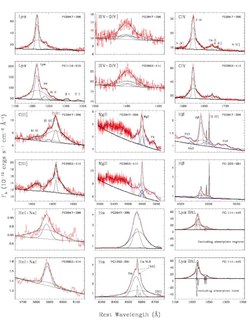
Figure 3: Model fitting to the emission lines. Two objects are shown for each line region. Shown with the data are the fitting results (thick solid lines), the local continua and individual components of the model (thin lines). The last two panels (lower-right corner) show ${\rm Ly}{\alpha}$ region of PG 1114+445, where the BAL features are excluded (upper) and modeled (lower) in the fitting, respectively. [See the electronic edition of the Journal for a color version of this figure and for plots of the complete sample (Figures 3.1–3.16)]

For each of several emission-line regions, we fit simultaneously a local power-law continuum and different emission-line components, using $\chi^{2}$ minimization within the IRAF package specfit (Kriss, 1994). Figure 3 shows examples of the fitting in different regions. We used a narrow and a broad Gaussian component to fit each strong, broad emission line. A velocity shift is allowed between the two components to account for the asymmetry of the line profile. For ${\rm H}{\alpha}$ and ${\rm H}{\beta}$, we have also included a third Gaussian component to account for the obvious NLR emission on top of the broad-line profile for several objects. For weak or narrow emission lines, one Gaussian component is used in the fitting.

We used symmetric Gaussian profiles, so each profile has three parameters: flux, width, and central wavelength. In order to avoid too many free parameters, for each emission-line region we assume the same width for similar components of different lines, tie together the wavelengths of some lines based on their laboratory wavelengths, and assume line intensity ratios for some lines based on their statistical weights. We list in Table 4 all the free and dependent parameters in each region and how the parameters are related. For example, in the ${\rm H}{\beta}$ region, [O iii] $\lambda$4959 has the same width and 1/3 of the flux of [O iii] $\lambda$5007; its wavelength is tied to that of [O iii] $\lambda$5007 (see also Kriss, 1994).

We have included Fe templates to account for the complicated Fe emission only in the optical ${\rm H}{\beta}$ region and UV Mg ii regions. Both the optical Fe ii template (Boroson & Green, 1992) and the UV Fe template (Vestergaard & Wilkes, 2001) were derived from the spectra of the narrow-line quasar I Zw 1. These templates were allowed to vary in both intensity and broadening to match the Fe emission in different objects, and they are fitted simultaneously with the local power-law continuum and emission-line components in specfit. In doing so, we assume that the Fe emission is above a power-law continuum, same assumption as these templates were derived. Iron can also be important in and near the red wing of C iv and introduces uncertainty in the related measurements for C iv. We discuss this in §3.4.

Figure 3 shows examples of our fitting results and individual components in each region. We also show our treatment of broad absorption lines or deep absorption features, in the lower right of the figure. There is obvious strong absorption of ${\rm Ly}{\alpha}$, C iv, or Si iv in three objects (PG1001+054, PG1114+445, PG1411+442). We attempted to fit the affected regions in two ways. First, we excluded the absorbed regions before fitting; second, we fit the region, including additional absorption Gaussian profiles at the absorption positions. The two methods give consistent results and we use the results from the first method in the following analyses.

Our fitting process separates the blended lines, but with possible large uncertainties because of uncertainties in continuum fitting and our assumptions about the relationships between different lines (Table 4), e.g., same width for two lines. This affects the weak lines the most and their fluxes are less reliable. They are used only to understand and remove their contribution on the strong lines. Even for some strong lines, although we define different emission lines in the region, we cannot really deblend them without arbitrary assumptions. Therefore, we present some measurements of just the total blend, such as Si iv+O iv] $\lambda$1400 and Na i+He i $\lambda$5876.

For all individual broad lines other than ${\rm H}{\beta}$ and ${\rm H}{\alpha}$, we use two Gaussian profiles at most and do not include an NLR component. This sometimes cannot fit the narrow peak for some lines. These peaks could indicate an NLR component, but without other supporting evidence, we cannot identify or separate them from the broad components. In fact, the lack of a ${\rm H}{\beta}$ NLR-like (or [O iii]-like) peak for C iv has led to a commonly accepted view that the NLR component of C iv is very weak, if not absent (e.g., Wills et al., 1993; Vestergaard & Peterson, 2006), although some studies (e.g., Sulentic & Marziani, 1999) claim a relatively strong C iv NLR component by allowing a fitted component generally much broader than [O iii]. Whether those residual peaks in our fitting are a NLR component or not, they contribute very little to the total flux of the strong emission lines. The FWHM might have been overestimated a little if there is a residual peak but no real NLR emission, but the uncertainty is still within the error of the measurements (§3.4). Our overall fit for each region is acceptable in terms of deblending and obtaining profile parameters of strong emission lines. These fits can be assessed by inspection of Figure 3.

Emission-line flux, EW and profile parameters are derived from the fitting results. For an emission line with a single Gaussian profile, the calculations are straightforward. For a strong broad emission line with two Gaussian profiles in the fitting, we add the two profiles and local continuum to form a model spectrum of the emission line region (excluding an NLR component) and then derive the parameters from the resulting model. EW is calculated using the line flux and the fitted local continuum at the emission line wavelength and then transformed to the rest-frame. All the line velocity shifts are for the peak of the model line profile and relative to the systemic redshift. FWHM and asymmetry are also derived from the emission line model. We define a line asymmetry parameter (De Robertis, 1985; Boroson & Green, 1992; Corbin & Boroson, 1996),

$$\mbox{Asymm}=\frac{\lambda_{c}(\frac{3}{4})-\lambda_{c}(\frac{1}{4})}{\mbox{FWHM}},$$

where $\lambda_{c}(\frac{3}{4})$ and $\lambda_{c}(\frac{1}{4})$ are the wavelength centers of cuts at $\frac{3}{4}$ and $\frac{1}{4}$ of the line peak flux density. A positive value indicates excess light in the blue wing of an emission line.

We provide the measurements of all strong emission lines in Table 5–10. The uncertainty of the measurements is discussed in §3.4.

3.3 Small Blue Bump

AGN UV-optical continuum spectra usually show a bump between 2000 Å and 4000 Å. This is referred as the “Small Blue Bump” (SBB) and consists mainly of unresolved Fe blends and Balmer continuum. Although we include the Fe template in fitting the Mg ii region, the UV Fe emission estimated is not complete due to the cutoff of the template at $\sim$3000Å. About 1/3 of the SBB above 3000Å is missing in the template, and the local continuum for Mg ii can also be affected in the fitting. We therefore attempt to measure the SBB directly by integrating the spectrum between 2220 and 4010 Å above a continuum and then subtracting the contribution of Mg ii using its fitting results.

We have tried different continua. The first one is the global UV-optical continuum defined by $\alpha_{{UVO}}$, but it is likely the SBB flux is overestimated (Fig. 4) because the continuum is defined over a wider wavelength range. We then define a local power-law continuum by connecting the spectrum between 2220 and 4010Å. In many cases, this underestimates the SBB. Although either can consistently give us a good estimate of the SBB for the whole sample and both have a large uncertainty, the estimates are simply related and both can roughly represent the SBB. More likely, they can be treated as the upper and lower limits of the SBB flux (Table 9).

3.4 Measurement Uncertainties

Since all our spectra are have high S/N ratio, the formal error in the fitting process is not significant. The major error comes from the placement of the local continuum in each emission-line region. Therefore, in order to estimate the uncertainties of the measured quantities, we adopt a method similar to Laor et al. (1994b, 1997a). We change the best-fit local continuum level by $1\sigma$ error at both ends of the local emission-line fitting region, build new model line profiles, and re-calculate the quantities (§3.2). We start from the best-fit local continuum fluxes $F_{left}$ and $F_{right}$ at both ends of a local continuum region. The $1\sigma$ errors of the continuum fluxes are measured at these two wavelengths as $\sigma_{left}$ and $\sigma_{right}$, respectively. Between $F_{left}\pm\sigma_{left}$ and $F_{right}\pm\sigma_{right}$, we have 4 combinations of the new local continuum. We repeat the above calculations 4 times, compare with the best-fit results, and pick up the largest differences as the errors for each quantity. For EWs, corresponding new continua are used in the calculation. The errors are listed in Table 5–10.

The errors calculated for line velocity shifts $\Delta v$ are always very small ($<5\,{\rm km~{}s}^{-1}$), but the real uncertainty for velocity shift results from the uncertainty of the redshifts defined and measured using [O iii] $\lambda$5007 (§2.3.4). The redshift measurement uncertainty can be roughly evaluated from the velocity shift of [O iii] $\lambda$5007 (Table 7), which is supposed to be zero.

For spectral indices, we use the same method to estimate their uncertainties. We note that another possibly important source of error for $\alpha_{{UVO}}$ comes from the Galactic reddening correction (§2.3.3). We do not attempt to estimate this error because of the lack of errors of E(B-V) for individual objects.

Blended iron emission causes complication in measuring other emission lines. We have used Fe templates to fit and remove the Fe emissions in the ${\rm H}{\beta}$ and Mg ii regions where Fe is strong, but we do not include the Fe template in the C iii] and C iv regions, where Fe can sometimes be important. Assuming the iron intensities in the Mg ii and C iv regions scale together, and using the fitting results from the Mg ii region and the same UV Fe template, we estimate the Fe contribution within $3\sigma_{broad}$ around the C iv line center, where $3\sigma_{broad}$ is the Gaussian $\sigma$ of the C iv broad Gaussian component, which mainly models the line wings. We found that the Fe is only $1.9\%$ of the total C iv flux on average, and $4.1\%$ for the worst case. In fact, in the fitting process of the C iv region, part of the Fe in the C iv red wing has been treated as pseudo-continuum and is not included in the measured C iv flux. Therefore, the uncertainty in C iv flux caused by Fe should be less than $4\%$ for all objects.

4 Estimation of Physical Parameters

We have estimated the black hole mass and accretion rate using the empirical method developed from reverberation mapping studies (Kaspi et al., 2000; Peterson et al., 2004). Assuming virial motion of the BLR,

$$M_{BH}=R_{BLR}\ v^{2}/G.$$ (1)

where velocity dispersion $v$ is estimated from ${\rm H}{\beta}$ line width, $v=\sqrt{3}/2\ \mbox{FWHM}({\rm H}{\beta})$, and the size of the BLR $R_{BLR}$ has an empirical relationship with luminosity (Kaspi et al., 2000),

$$R_{BLR}=32.9^{+2.0}_{-1.9}\left[\frac{\lambda L_{\lambda}(5100\mbox{\AA})}{10^{44}\mbox{erg s}^{-1}}\right]^{0.70\pm 0.033}\mbox{ light days}.$$ (2)

$\lambda L_{\lambda}(5100\mbox{\AA})$ is calculated using the fitted local continuum in the ${\rm H}{\beta}$ region and our adopted cosmology ($\Lambda=0,\ H_{0}=75\,{\rm km~{}s}^{-1}\mbox{Mpc}^{-1},q_{0}=0.5$). Similarly, we also obtain a UV luminosity $L_{1549}$=$\lambda L_{\lambda}(1549\mbox{\AA})$, using the local continuum in the C iv region at 1549 Å.

Following Kaspi et al. (2000), we define the bolometric luminosity $L_{Bol}$=9 $\lambda L_{\lambda}$(5100Å). Knowing the black hole mass, we can then estimate the Eddington accretion ratio, $L_{Bol}/L_{Edd}$, where $L_{Edd}=1.25\times 10^{38}(M_{\rm BH}/M_{\odot})$. The bolometric luminosity defined here is only an estimate of the true bolometric luminosity. Different scaling factors for monochromatic luminosity exist, e.g., $L_{Bol}$$\approx$13.2 $\lambda L_{\lambda}$(5400Å) (Elvis et al., 1994). Shang et al. (2005) estimated $L_{Bol}$ for a sample with good far-UV-optical spectra and found $L_{Bol}$$\approx 1.5\times$ 9 $\lambda L_{\lambda}$(5100Å). Using photoionization modeling to determine the ionizing continuum, Wandel et al. (1999) deduce $L_{Bol}$$\approx$10 $\lambda L_{\lambda}$(5100Å). Recently, using multi-wavelength data, Richards et al. (2006a) show $L_{Bol}$=($10.3\pm 2.1)$ $\lambda L_{\lambda}$(5100Å), and point out that deriving a bolometric luminosity from a single optical luminosity can lead to errors as large as 50%. We note that our adopted $L_{Bol}$ may have large uncertainty, but the relative error within the sample is smaller. We list these derived parameters in Table 11.

5 Properties of Emission Line Profiles

We compare here the profile properties of lines arising from different atomic transitions, and present the correlations of their FWHM, velocity shift, and asymmetry parameter. We leave more detailed analyses to Paper II (Wills et al., 2007). We denote the Pearson correlation coefficient by $r$ and the two-tailed probability of a correlation arising by chance, by $p$. Note that we have previously discussed the line-width correlations based on different line measurements, in Wills et al. (2000).

5.1 Line Width

As illustrated clearly in Figure 5, ${\rm H}{\alpha}$ FWHM has the strongest correlation with ${\rm H}{\beta}$ FWHM. The scatter of the correlations with ${\rm H}{\beta}$ FWHM gets larger for Mg ii and C iii], and the correlation virtually disappears for ${\rm Ly}{\alpha}$ and C iv. However, a correlation between ${\rm Ly}{\alpha}$ and C iv FWHMs exists ($r=0.81,p<10^{-5}$). Similar results have been noticed before, e.g., Corbin & Boroson (1996) also found that the FWHMs of C iv and ${\rm Ly}{\alpha}$ are more strongly correlated with each other than with ${\rm H}{\beta}$. In QSOs’ photoionized regions the ${\rm Ly}{\alpha}$ behavior is expected because a significant fraction is emitted from the high-ionization region along with CIV. Therefore we treat ${\rm Ly}{\alpha}$ as a high-ionization line.

We also notice that C iv and ${\rm Ly}{\alpha}$ are not necessarily broader than ${\rm H}{\beta}$. This seems to argue against a simple radially stratified ionization structure of BLR as suggested by reverberation mapping studies (e.g., Peterson et al., 1991; Korista et al., 1995), but it is more likely that the total line width is affected by a wind component. We discuss this more in §5.4.

We note the possible problem with ${\rm Ly}{\alpha}$ measurements here. When fitting ${\rm Ly}{\alpha}$ region, we assume that N v has the same profile as ${\rm Ly}{\alpha}$ and tie its wavelength to ${\rm Ly}{\alpha}$. If the assumptions are wrong, it will affect the measurements of ${\rm Ly}{\alpha}$. The ${\rm Ly}{\alpha}$ line velocity shift is affected little because it is measured from the ${\rm Ly}{\alpha}$ line peak, however, the line width can be affected when N v is strong and the asymmetry parameter can be affected if N v is not correctly de-coupled from the ${\rm Ly}{\alpha}$ red wing. Without knowing the true profile of N v, this situation remains true for any attempt of de-blending ${\rm Ly}{\alpha}$ and N v under assumptions.

5.2 Line Peak Shift

We plot the distributions of emission-line velocity shifts in Figure 6 and list their statistics in Table 12. It is clear that C iv shows significant blueshifts. This agrees with the results from a large sample in Baskin & Laor (2005) in general, although the shift parameter is defined in the units of FWHM there. There is evidence that ${\rm Ly}{\alpha}$ and Mg ii are also blueshifted, but not as much as C iv. ${\rm H}{\alpha}$ and ${\rm H}{\beta}$ show small redshifts, but it seems there is not a preferred direction for C iii] velocity shift, suggesting that C iii] may also be good for defining the QSO redshift if narrow lines are not available. However, we note that the wavelength of C iii] can be measured accurately enough only when the broad emission lines in this spectral region are sufficiently narrow to allow a decomposition. Although the dispersion of line shifts is large, it seems, from blueshift to redshift, that a sequence is formed for C iv, ${\rm Ly}{\alpha}$, Mg ii, C iii], ${\rm H}{\beta}$, and ${\rm H}{\alpha}$, suggesting an ionization level dependence. This agrees with some earlier studies (e.g., Gaskell, 1982; Corbin, 1990; Tytler & Fan, 1992), but not others (e.g., Laor et al., 1995).

Our correlation analyses (Table 13) further show that the shifts of C iv and ${\rm Ly}{\alpha}$ are correlated ($r=0.81,p=4.9\times 10^{-6}$), and those of ${\rm H}{\alpha}$ and ${\rm H}{\beta}$ are also correlated ($r=0.62,p=0.002$), but the shifts of C iv and ${\rm Ly}{\alpha}$ do not seem to be related to that of ${\rm H}{\alpha}$ or ${\rm H}{\beta}$. In terms of the correlation coefficients, Mg ii and C iii] seems to be related to ${\rm H}{\alpha}$ and ${\rm H}{\beta}$ more closely than to C iv and ${\rm Ly}{\alpha}$.

5.3 Asymmetry

We have measurements of asymmetry for only four emission lines. They appear to form two groups (Fig. 7). ${\rm H}{\alpha}$ and ${\rm H}{\beta}$ show little or no asymmetry, while C iv and ${\rm Ly}{\alpha}$ show significant asymmetry with excess flux in the blue wing. These agree with the results of C iv and ${\rm H}{\beta}$ in Baskin & Laor (2005), but we also show that C iv and ${\rm Ly}{\alpha}$ asymmetries are marginally correlated ($r=0.53,p=0.01$, Table 14), and the asymmetry parameters for ${\rm H}{\alpha}$ and ${\rm H}{\beta}$ show little correlation ($r=0.43,p=0.05$).

5.4 Discussion of Line Profiles

The difference between high and low-ionization line profiles has been investigated extensively in early studies (e.g., Gaskell, 1982; Wilkes, 1984; Espey et al., 1989; Corbin, 1991; Tytler & Fan, 1992; Laor et al., 1995; Sulentic et al., 1995; Wills et al., 1995; Corbin & Boroson, 1996; Marziani et al., 1996; Vanden Berk et al., 2001; Richards et al., 2002). It is well known that, compared with low-ionization lines, high-ionization lines tend to have large blue shifts and asymmetries with stronger blue wings. Our data give us the advantage of comparing, for each QSO, all the strong UV and optical emission lines of different ionization stage at essentially the same epoch.

In our sample, the decreasing significance of FWHM correlations with ${\rm H}{\beta}$ FWHM from low-ionization lines to high-ionization lines suggests that, within the broad line emitting region, kinematics is a function of ionization. This is also supported by the rough sequence of line peak shifts and asymmetries with ionization stage. All the evidence show two distinct groups of lines and a possible third group in between. High-ionization lines C iv and ${\rm Ly}{\alpha}$ are clearly distinct from low-ionization ${\rm H}{\beta}$ and ${\rm H}{\alpha}$, while Mg ii and C iii] seems intermediate.

Systematically asymmetric line profiles and shifts must be the result of radial motions, together with obscuration (optical depth, dust) (e.g. Ferland et al., 1979). For example, stronger blue wings and blueshifts could be the result of nuclear outflow, with emission from the far side of the center suppressed. Stronger blue wings could also be the result of flow towards the nucleus with anisotropic emission stronger from the more highly ionized regions facing the continuum source. Richards et al. (2002) and Richards (2006b) interpreted the range of CIV profiles (blueshifts) in a large SDSS sample as a combination of dust obscuration and orientation.

While it seems that the kinematics of the BLR may be related to the ionization structure, our sample shows that the high ionization C iv line is broader than the low ionization ${\rm H}{\beta}$ line in only about half the objects. This appears to contradict a simple radially stratified ionization structure of the BLR indicated by reverberation mapping, in which high-ionization clouds are closer to the ionizing source and therefore have higher (virial) velocity dispersion (e.g., Peterson et al., 1991; Korista et al., 1995). However, the measured line widths may not simply be a function of Keplerian velocity, and they can include additional velocity components contributed by wind, outflows etc. We previously noted that narrow line Seyfert 1 (NLS1) objects with ${\rm H}{\beta}$ FWHM $<2000$ ${\rm km~{}s}^{-1}$showed ${\rm Ly}{\alpha}$ and C iv FWHM $>$ ${\rm H}{\beta}$ FWHM, and argued for the presence of a high-ionization outflow in NLS1s (Wills et al., 2000). Baskin & Laor (2005) have analyzed a larger sample and shown that ${\rm H}{\beta}$ is broader than C iv when ${\rm H}{\beta}$ FWHM $>$ 4000 ${\rm km~{}s}^{-1}$. They attribute this partly to an outflowing wind component in the BLR, as we suggested for our sample (Wills et al., 2000). Vestergaard & Peterson (2006) have re-analyzed the Baskin & Laor sample, culling the less-reliable data, and agree that there is probably a strong outflowing wind in NLS1s (see also Vestergaard, 2004). Detailed studies of individual NLSy1s have shown that high-ionization lines have a clear blueshifted wind component, indicated by the large flux excess in their blue wing (Leighly & Moore, 2004; Leighly, 2004; Yuan et al., 2007).

${\rm H}{\beta}$ FWHM and ${\rm H}{\alpha}$ FWHM have been used as a measure of BLR velocity dispersion to estimate the black hole mass (e.g., Peterson, 1993; Kaspi et al., 2000; Greene & Ho, 2005). Mg ii has also been used for estimating black hole mass at higher redshifts (McLure & Jarvis, 2002), and it seems to be valid as the FWHMs of ${\rm H}{\beta}$ and Mg ii are strongly correlated. However, although it also seems to work statistically, the use of C iv (e.g., Vestergaard, 2002) may introduce significant uncertainty. This is suggested by the evidence for outflow in NLS1s, and is the reason Vestergaard & Peterson (2006) exclude NLS1s from their investigation of the use of C iv FWHM to estimate black hole mass. Asymmetry and line shifts occur in C iv, other high-ionization lines (§5), and to a lesser extent, in ${\rm H}{\beta}$, and not just for NLS1s. This suggests that further refinement in black hole mass determinations may be possible after accounting for obscuration and optical depth effects (by measuring the width of the unsuppressed wing about the expected systemic velocity), or taking into account additional non-virial (outflow) motions (measuring the narrower virial wing about the expected systemic velocity). Vestergaard & Peterson (2006) note that, statistically, the uncertainties in the above effects for non-NLS1s are within the uncertainties of single-epoch width measurements, thus validating the use of C iv for black hole mass measurements. However, for objects with an extreme outflow component in the line profile (e.g., the aforementioned NLS1s), C iv still could not be used in the black hole mass measurements.

6 SUMMARY

1. We present quasi-simultaneous UV and optical spectra covering a broad wavelength range from below ${\rm Ly}{\alpha}$ to at least ${\rm H}{\alpha}$ for an essentially complete sample of low-redshift quasars. We measured the UV-optical continuum slopes (power-law). Line widths, shifts, and asymmetries are also measured for all strong emission lines and results presented.

2. Our analyses of UV-optical emission line profiles indicate radial motions and anisotropic line emission (wind, optical depth effects or dust obscuration) that is related to the ionization structure, thus excluding a simple radially stratified ionization structure, with gas in virial motion.

   We will present detailed correlation analyses and multi-variate analyses of all the spectral parameters in a separate paper (Wills et al., 2007).

Appendix A Notes on Data for Individual Objects

The UV spectrum of each object is either from $HST$ archives or from our own observations, and in general the optical spectra were obtained at McDonald Observatory. There are a few cases where we use data from other sources (see also Figure 1 and Table 2). Wavelengths here are all in the observed frame.

PG1048+342

Due to the very low flux measured from IUE data, this object would have required an unreasonable amount of HST time to observe, and therefore the observation was not proposed. It turned out later that the IUE data spectrum was weak, probably because of a pointing problem. This is the object that is in the complete sample of Laor et al. (1994b, 1997a), but is not included in the analyses in this paper.

PG1116+215

Most data (1668–8231Å) are from our new observations (both $HST$ and McDonald), while a small part of the spectrum (1239–1774Å, including ${\rm Ly}{\alpha}$) is from the $HST$ archive.

PG1202+281

Archival HST UV data in the wavelength range 2400–3277Å are also used to increase the signal-to-noise ratio. The flux density of this spectrum agrees very well with the new $HST$ spectrum, although this object is highly variable (Sitko et al., 1993, and references therein).

PG1226+023 (3C273)

Some optical data (3200–8183Å) are from 1981 and 1988 observations using the UVITS spectrograph and image dissector scanner (IDS) on the 2.7m telescope at McDonald Observatory (Wills, Netzer, & Wills, 1985).

PG1512+370

The blue part of our optical spectrum (shown in Figure 1, 3201–5631Å) is not used due to poor quality, instead, data are from observations by Jack Baldwin (3174–5570Å), Boroson and Green (BG92) (6120–7052Å) and Bev Wills’ archival McDonald IDS data (5567–6230Å).

PG1543+489

We were not able to obtain the UV spectrum between 2307–3200Å (G190H) because the data were supposed to be obtained for another $HST$ proposal before ours, but were never obtained. We also do not have data for part of its ${\rm H}{\alpha}$ red wing (Fig. 2).

Figure 1: Summary of observations and wavelength coverage. Object names and redshifts are labeled on the left. Each horizontal line indicates one individual spectrum; dashed lines indicate archival data. Different colors indicate different observing runs and instruments, Large Cassegrain Spectrograph (LCS) or Electronic Spectrograph 2 (ES2). The small triangles mark, from left to right, the locations of ${\rm Ly}{\alpha}$, Mg ii, ${\rm H}{\beta}$, and ${\rm H}{\alpha}$. Some HST spectra extend to the optical. Duplicate spectra with the same wavelength coverage are all used in the final combination for each object (§2.3.3).

Figure 2: UV-optical spectra and fitted power-laws for different regions. The pairs of vertical dotted lines indicate the continuum windows used for fitting $\alpha_{{UVO}}$ ($\sim$1200–5500Å) and $\alpha_{{Ored}}$ ($\sim$5500–8000Å) (Table 3). The HST spectra are oversampled and have been rebinned to a resolution of 2Å for display purpose. The flux is still in observed frame. [See the electronic edition of the Journal for a color version of this figure.]

Figure 2: Continued

Figure 2: Continued

Figure 4: Illustration of different continua defined for estimating the flux of the Small Blue Bump (§3.3). The global power-law ($\alpha_{{UVO}}$, dashed-line) is shown as well as the local power-law continuum (solid thick line) defined between 2220 and 4010 Å. The vertical lines indicate the flux integration region for the Small Blue Bump and Mg ii has been modeled and subtracted. Mg ii model and its fitting continuum are overplotted (solid thin line). Note that Mg ii fitting continuum is not good to estimate the flux of the Small Blue Bump (§3.3),

Figure 5: Emission line FWHM vs. those of ${\rm H}{\beta}$ and C iv. The dotted lines indicate equal FWHMs. Note that we do not have C iii] measurement for PG 1543+489.

Figure 6: Distribution of emission-line shift for the whole sample (solid line) and for leaving out 3 objects (dotted line) whose redshifts are not measured using [O iii]. Positive values indicate redshift. The vertical dashed lines indicate the median values for the whole sample.

Figure 7: Distribution of emission-line asymmetry. See §3.2 for definition of the asymmetry parameter. Positive values indicate excess flux in the blue wing.

Table 1: The Sample

Object	Other Name	$z$	$m_{B}$	$\alpha_{\rm X}$	$R$	E(B-V)
PG0947+396		0.2056	16.40	$-$1.510	0.25	0.019
PG0953+414		0.2341	15.05	$-$1.570	0.44	0.013
PG1001+054		0.1603	16.13	$-$2.800	0.5	0.016
PG1114+445		0.1440	16.05	$-$1.550	0.13	0.016
PG1115+407		0.1541	16.02	$-$1.890	0.17	0.016
PG1116+215	TON 1388	0.1759	15.17	$-$1.730	0.72	0.023
PG1202+281	GQ COM	0.1651	15.02	$-$1.220	0.19	0.021
PG1216+069		0.3319	15.68	$-$1.360	1.65	0.022
PG1226+023	3C 273	0.1575	12.86	$-$0.942	1138	0.021
PG1309+355	TON 1565	0.1823	15.45	$-$1.510	18	0.012
PG1322+659		0.1675	15.86	$-$1.690	0.12	0.019
PG1352+183	PB 4142	0.1510	15.71	$-$1.524	0.11	0.019
PG1402+261	TON 182	0.165	15.57	$-$1.930	0.23	0.016
PG1411+442	PB 1732	0.0895	14.99	$-$1.970	0.13	0.008
PG1415+451		0.1143	15.74	$-$1.740	0.17	0.009
PG1425+267	TON 202	0.3637	15.67	$-$0.940	53.6	0.019
PG1427+480		0.2203	16.33	$-$1.410	0.16	0.017
PG1440+356	Mrk 478	0.0773	15.00	$-$2.080	0.37	0.014
PG1444+407		0.267	15.95	$-$1.910	$\lesssim$0.08	0.014
PG1512+370	4C 37.43	0.3700	15.97	$-$1.210	190	0.022
PG1543+489		0.400	16.05	$-$2.110	0.15	0.018
PG1626+554		0.1317	16.17	$-$1.940	0.11	0.006

Table 2: Observing Time, Observing Time Gap, and Scaling Factor

	Observing Date (UT)					Observing Time Gap (days)					Scaling Factor
		Ground-based					Ground-based					Ground-based
Object	HST	Blue	Middle	Red		HST	Blue	Middle	Red		HST	Blue	Middle	Red
PG0947+396	1996-05-06	1996-04-19	1996-04-17			19	2	0			0.97	0.99	1
			1996-04-18					1					1.04
PG0953+414	1991-06-18	1996-04-24	1996-05-13	1997-02-11		-1791	-19	0	274		1.29	0.94	1	1.08
	1991-11-05	1996-04-25				-1651	-18				1.29	1.22
		1997-02-10					273					0.81
PG1001+054	1997-01-15	1997-02-10	1997-02-13	1997-02-16		-26	0	3	6		0.93	1	1.05	0.97
PG1114+445	1996-05-13	1996-04-19	1996-04-17			24	0	-2			1.08	1	1.03
PG1115+407	1996-05-19		1996-04-18	1997-02-16		31		0	304		1.16		1	0.97
			1997-02-13					301					1.02
PG1116+215	1996-05-26	1996-05-12	1996-05-13			13	-1	0			1.00	0.98	1
	1993-02-19					-1179					1.00
PG1202+281	1996-07-21	1996-04-19	1996-04-17	1997-02-16		-210	-303	-305	0		1.04	1.02	1.05	1
	1992-12-14	1997-02-15	1996-04-18			-1525	-1	-304			1.04	1.00	1.00
PG1216+069	1993-03-16	1996-04-24	1996-05-13	1996-05-11		-1152	-17	2	0		0.75	0.67	1.00	1
PG1226+023	1991-01-14	1981,1988	1996-02-17	1997-02-17		-2226		-366	0		0.72	0.89	0.77	1
PG1309+355	1996-05-20	1996-05-12	1996-04-17			33	25	0			1.00	0.95	1
			1996-05-10					23					1.05
PG1322+659	1997-01-19	1997-02-15	1996-04-18	1997-02-16		-27	0	-303	1		0.98	1	0.82	1.03
		1996-04-19					-302					0.79
PG1352+183	1996-05-26	1996-05-12	1996-04-18			38	24	0			0.99	1.01	1
			1996-05-10					22					1.09
PG1402+261	1996-08-25	1996-05-12	1996-05-10	1996-05-11		105	0	-2	-1		1.00	1	1.14	1.03
PG1411+442	1992-10-03	1996-04-19	1996-05-13			-1318	-24	0			1.66	1.01	1
PG1415+451	1997-01-02	1997-02-09	1997-02-13	1997-02-11		-42	-4	0	-2		1.01	1.10	1	2.26
		1997-02-10					-3					1.12
PG1425+267	1996-06-29		1996-04-17	1996-05-11		73		0	24		1.15		1	1.02
			1996-05-19					32					1.08
PG1427+480	1997-01-07	1997-02-10	1997-02-13	1997-02-11		0	34	37	35		1	1.01	0.98	1.17
PG1440+356	1996-12-05	1997-02-10	1997-02-13	1997-02-11		0	67	70	68		1	0.98	0.93	1.03
PG1444+407	1996-05-23	1996-05-12	1996-05-13	1996-05-11		10	-1	0	-2		0.74	1.00	1	1.01
	1992-09-05					-1346
PG1512+370	1992-01-26	1994-10-10	1990-09-20	1997-02-17		-1849	-861	-2342	0		0.64	scaled	scaled	1
			1984-05-31					-4645					scaled
PG1543+489	1995-05-14	1996-04-25	1996-04-18	1996-05-11		-340	7	0	23		1.00	1.11	1	0.98
PG1626+554	1996-11-19					0					1.00

Note. — See Figure 1 for wavelength coverage for each observation.

Table 3: Spectral Indices

	1200–5500Å region				$\sim$5500–8000Å region
Object	Win	$f_{1000}$	$\alpha_{{UVO}}$		Win	$f_{1000}$	$\alpha_{{Ored}}$	$\Delta\alpha$	$f_{\nu}$(1keV)	$\alpha_{\rm X}$	$\alpha_{ox}$
PG0947	a,d	$17.6\pm 0.9$	$-1.76\pm 0.04$		d,e	$\phantom{0}2.6^{+2.0}_{-1.1}$	$-0.66\pm 0.32$	$-1.10$	7.64	$-1.51$	$-1.42$
PG0953	a,d	$26.5\pm 1.1$	$-1.69\pm 0.03$		d,f	$18.9^{+6.4}_{-4.8}$	$-1.50\pm 0.16$	$-0.19$	9.33	$-1.57$	$-1.47$
PG1001	b,d	$6.3\pm 0.4$	$-1.45\pm 0.06$		d,f	$\phantom{0}4.9^{+6.3}_{-2.7}$	$-1.30\pm 0.45$	$-0.15$	0.05	$-2.80$	$-2.29$
PG1114	a,d	$7.7\pm 0.3$	$-0.88\pm 0.03$		d,f	$\phantom{0}6.9^{+2.3}_{-1.7}$	$-0.81\pm 0.16$	$-0.06$	1.91	$-1.55$	$-1.65$
PG1115	a,d	$22.8\pm 1.2$	$-1.83\pm 0.04$		d,f	$\phantom{0}2.8^{+0.9}_{-0.7}$	$-0.60\pm 0.15$	$-1.23$	3.79	$-1.89$	$-1.61$
PG1116	a,d	$68.0\pm 2.0$	$-2.03\pm 0.02$		d,f	$10.2^{+2.9}_{-2.2}$	$-0.93\pm 0.14$	$-1.10$	13.10	$-1.73$	$-1.54$
PG1202	a,d	$3.4\pm 0.3$	$-0.97\pm 0.07$		d,f	$\phantom{0}1.3^{+0.5}_{-0.4}$	$-0.42\pm 0.18$	$-0.55$	9.88	$-1.22$	$-1.19$
PG1216	a,d	$10.5\pm 0.4$	$-1.34\pm 0.03$		d,f	$\phantom{0}5.4^{+2.5}_{-1.7}$	$-0.95\pm 0.21$	$-0.38$	7.93	$-1.36$	$-1.37$
PG1226	a,d	$291.6\pm 4.0$	$-1.79\pm 0.01$		d,f	$62.3^{+11.8}_{-9.9}$	$-0.90\pm 0.10$	$-0.89$	178.00	$-0.94$	$-1.29$
PG1309	a,d	$16.1\pm 0.6$	$-1.26\pm 0.02$		d,f	$13.5^{+3.3}_{-2.7}$	$-1.15\pm 0.12$	$-0.10$	3.02	$-1.51$	$-1.63$
PG1322	a,d	$12.7\pm 0.4$	$-1.51\pm 0.02$		d,f	$\phantom{0}7.9^{+2.3}_{-1.8}$	$-1.24\pm 0.14$	$-0.27$	8.19	$-1.69$	$-1.41$
PG1352	a,d	$16.3\pm 1.1$	$-1.76\pm 0.05$		d,f	$\phantom{0}4.4^{+5.5}_{-2.4}$	$-1.01\pm 0.43$	$-0.75$	7.85	$-1.52$	$-1.40$
PG1402	a,d	$37.6\pm 2.3$	$-1.92\pm 0.04$		d,f	$\phantom{0}9.0^{+2.4}_{-1.9}$	$-1.10\pm 0.13$	$-0.82$	9.86	$-1.93$	$-1.53$
PG1411	a,d	$37.9\pm 2.8$	$-1.36\pm 0.05$		d,f	$28.3^{+5.7}_{-4.8}$	$-1.19\pm 0.10$	$-0.17$	0.31	$-1.97$	$-2.19$
PG1415	a,d	$15.5\pm 0.8$	$-1.39\pm 0.04$		d,f	$\phantom{0}5.4^{+2.1}_{-1.5}$	$-0.78\pm 0.18$	$-0.62$	3.28	$-1.74$	$-1.62$
PG1425	b,d	$7.0\pm 0.3$	$-1.50\pm 0.04$		d,e	$\phantom{0}3.3^{+4.4}_{-1.9}$	$-1.07\pm 0.47$	$-0.43$	0.85	$-0.94$	$-1.60$
PG1427	a,d	$12.1\pm 0.6$	$-1.80\pm 0.03$		d,f	$\phantom{0}4.0^{+1.6}_{-1.1}$	$-1.16\pm 0.18$	$-0.64$	3.26	$-1.41$	$-1.48$
PG1440	a,d	$60.4\pm 2.3$	$-1.55\pm 0.03$		d,f	$25.3^{+2.9}_{-2.6}$	$-1.04\pm 0.06$	$-0.50$	20.20	$-2.08$	$-1.56$
PG1444	a,d	$15.0\pm 0.6$	$-1.65\pm 0.03$		d,f	$14.1^{+4.5}_{-3.4}$	$-1.61\pm 0.15$	$-0.03$	2.89	$-1.91$	$-1.62$
PG1512	b,d	$7.5\pm 0.2$	$-1.76\pm 0.04$		d,e	$\phantom{0}2.0^{+11.5}_{-1.7}$	$-0.99\pm 1.05$	$-0.77$	6.00	$-1.21$	$-1.28$
PG1543	a,d	$8.5\pm 0.7$	$-1.65\pm 0.06$		d,e	$\phantom{0}5.8^{+11.1}_{-3.8}$	$-1.44\pm 0.61$	$-0.22$	1.02	$-2.11$	$-1.72$
PG1626	a,d	$30.3\pm 1.4$	$-1.83\pm 0.05$		d,f	$10.1^{+14.6}_{-6.0}$	$-1.20\pm 0.49$	$-0.63$	12.80	$-1.94$	$-1.46$

Note. — $\alpha_{{UVO}}$ and $\alpha_{{Ored}}$ are rest-frame $\alpha_{\lambda}$ ($f_{\lambda}\propto\lambda^{{\alpha_{\lambda}}}$); $\alpha_{\rm X}$ and $\alpha_{ox}$ (between 2500Å and 2 keV) are rest-frame $\alpha_{\nu}$($f_{\nu}\propto\nu^{\alpha_{\nu}}$).

Table 4: Fitting Parameters for Emission Lines

			Gaussian	Gaussian Parameter			Flux
ID	Line	$\lambda$	Component	Flux	Center	FWHM	Ratio
1	${\rm Ly}{\alpha}$	1215.67	narrow	free	free	free
2			broad	free	free	free
3	NV	1238.81	narrow	free	1	1	1
4			broad	${\rm Ly}{\alpha}$ shape	2	2	1
5	NV	1242.80	narrow	3	3	3	1
6			broad	4	4	4	1
7	SiII	1260.42		free	1	free	0.33
8	SiII	1264.73		7	7	7	0.6
9	SiII	1265.02		7	7	7	0.07
10	OI	1302.17		free	1	7	1
11	OI	1304.87		10	10	10	1
12	OI	1306.04		10	10	10	1
13	CII	1335.31		free	1	10
1	Si iv	1396.75	broad	free	free	free	1
2			narrow	free	1	free	1
3	O iv]	1402.34	broad	1	1	1	1
4			narrow	2	2	2	1
1	N iv]	1486.50		free	free	free
2	C iv	1548.20	narrow	free	free	free	1
3			broad	free	free	free	1
4	C iv	1550.77	narrow	2	2	2	1
5			broad	3	3	3	1
6	He ii	1640.72	narrow	free	free	free
7			broad	free	6	3
8	O iii]	1660.80		free	1	free	0.29
9		1666.14		8	8	8	0.71
10	N iii]	1748.65		free	8	free	0.41
11		1752.16		10	10	10	0.14
12		1754.00		10	10	10	0.45
1	C iii]	1908.73	narrow	free	free	free
2			broad	free	1	free
3	Si iii]	1892.03	narrow	free	1	1
4			broad	C iii] shape	3	2
5	Al iii	1854.72		free	1	free	1
6	Al iii	1862.78		5	5	5	1
1	Mg ii	2795.53	narrow	free	free	free	2
2			broad	free	1	free	2
3	Mg ii	2802.71	narrow	1	1	1	1
4			broad	2	2	2	1
5	Fe	template		free	$\cdots$	free
1	${\rm H}{\beta}$	4861.32	narrow	free	free	free
2			broad	free	free	free
3			NLR	free	4	4
4	[O iii]	5006.84		free	free	free	3
5		4958.91		4	4	4	1
6	He ii	4685.65		free	1	1
7	Fe ii	template		free	$\cdots$	free
1	He i	5875.70	narrow	free	free	free
2			broad	free	1	free
1	${\rm H}{\alpha}$	6562.80	narrow	free	free	free
2			broad	free	free	free
3			NLR	free	free	4
4	[N ii]	6548.06		free	4	[O iii] width	1
5		6583.39		4	4	4	3
6	[S ii]	6716.47		free	4	4	1
7		6730.85		6	6	6	1

Note. — Each section separated by a horizontal line is for one emission line region. All parameters are related within the same region only unless noted.

Table 5: Parameters of Strong Emission Lines ${\rm Ly}{\alpha}$, N v, and Si iv+O iv] $\lambda$1400.

	Ly$\alpha$ $\lambda$1216						N v $\lambda$1240			Si iv $\lambda$1397 or O iv] $\lambda$1402
Object	Flux	EW	FWHM	$\Delta v$	Asymm		Flux	EW		Flux	EW	FWHM	$\Delta v$
PG0947	1275${}^{+75}_{-64}$	107.5${}^{+11.6}_{-10.6}$	3000${}^{+25}_{-25}$	$-165$	$-0.068^{+0.010}_{-0.014}$		68${}^{+92}_{-43}$	6.0${}^{+8.7}_{-8.0}$		75${}^{+48}_{-31}$	7.7${}^{+5.6}_{-5.1}$	5560${}^{+1170}_{-920}$	$105$
PG0953	2394${}^{+79}_{-69}$	125.5${}^{+9.2}_{-8.6}$	2500${}^{+15}_{-10}$	$-215$	$0.014^{+0.003}_{-0.005}$		310${}^{+126}_{-91}$	16.5${}^{+7.7}_{-7.1}$		121${}^{+52}_{-38}$	6.9${}^{+3.4}_{-3.1}$	5430${}^{+845}_{-750}$	$420$
PG1001	432${}^{+17}_{-14}$	107.7${}^{+10.6}_{-9.5}$	3350${}^{+55}_{-50}$	$-465$	$0.049^{+0.003}_{-0.002}$		215${}^{+30}_{-24}$	54.3${}^{+10.9}_{-9.8}$		52${}^{+13}_{-9}$	13.4${}^{+4.1}_{-3.8}$	3340${}^{+155}_{-155}$	$-1010$
PG1114	969${}^{+36}_{-31}$	146.7${}^{+12.6}_{-11.5}$	3040${}^{+15}_{-20}$	$250$	$0.095^{+0.006}_{-0.006}$		132${}^{+56}_{-40}$	20.1${}^{+9.8}_{-9.0}$		55${}^{+25}_{-18}$	8.7${}^{+4.5}_{-4.2}$	5815${}^{+1165}_{-920}$	$265$
PG1115	1140${}^{+109}_{-91}$	76.2${}^{+11.8}_{-10.7}$	3685${}^{+60}_{-65}$	$-185$	$0.235^{+0.029}_{-0.030}$		227${}^{+175}_{-108}$	15.7${}^{+13.6}_{-12.2}$		91${}^{+48}_{-34}$	7.1${}^{+4.3}_{-3.9}$	4665${}^{+850}_{-715}$	$-180$
PG1116	4379${}^{+171}_{-147}$	98.7${}^{+6.2}_{-5.9}$	4375${}^{+20}_{-30}$	$-385$	$-0.035^{+0.002}_{-0.002}$		777${}^{+268}_{-196}$	18.1${}^{+6.8}_{-6.5}$		262${}^{+70}_{-55}$	7.5${}^{+2.2}_{-2.1}$	5265${}^{+465}_{-420}$	$380$
PG1202	904${}^{+31}_{-27}$	382.7${}^{+62.0}_{-49.7}$	2650${}^{+10}_{-10}$	$-235$	$0.055^{+0.003}_{-0.003}$		138${}^{+49}_{-35}$	58.9${}^{+30.8}_{-24.6}$		49${}^{+16}_{-12}$	19.8${}^{+9.1}_{-7.7}$	4475${}^{+445}_{-410}$	$-1095$
PG1216	1005${}^{+31}_{-27}$	126.4${}^{+7.7}_{-7.2}$	2980${}^{+10}_{-10}$	$85$	$-0.063^{+0.002}_{-0.005}$		$\cdots$	$\cdots$		34${}^{+18}_{-12}$	5.1${}^{+2.9}_{-2.7}$	5960${}^{+875}_{-800}$	$400$
PG1226	9079${}^{+322}_{-278}$	43.8${}^{+2.1}_{-2.0}$	3165${}^{+15}_{-15}$	$-275$	$-0.065^{+0.005}_{-0.005}$		575${}^{+462}_{-267}$	2.9${}^{+2.4}_{-2.3}$		1293${}^{+579}_{-392}$	5.4${}^{+2.5}_{-2.5}$	5820${}^{+455}_{-430}$	$-380$
PG1309	1030${}^{+50}_{-43}$	81.1${}^{+7.0}_{-6.5}$	2070${}^{+15}_{-20}$	$480$	$0.379^{+0.008}_{-0.008}$		112${}^{+77}_{-51}$	8.9${}^{+6.7}_{-6.2}$		46${}^{+23}_{-15}$	4.1${}^{+2.2}_{-2.1}$	3840${}^{+505}_{-460}$	$-30$
PG1322	1106${}^{+24}_{-21}$	118.6${}^{+5.9}_{-5.6}$	2745${}^{+10}_{-10}$	$-50$	$0.105^{+0.005}_{-0.004}$		183${}^{+37}_{-29}$	20.1${}^{+4.7}_{-4.4}$		50${}^{+14}_{-11}$	6.1${}^{+1.9}_{-1.8}$	5640${}^{+515}_{-485}$	$-1170$
PG1352	1363${}^{+99}_{-84}$	124.5${}^{+18.9}_{-16.4}$	3035${}^{+50}_{-40}$	$-60$	$0.044^{+0.016}_{-0.013}$		159${}^{+155}_{-91}$	15.0${}^{+16.8}_{-14.6}$		87${}^{+59}_{-40}$	8.7${}^{+7.0}_{-6.1}$	5555${}^{+1650}_{-1225}$	$90$
PG1402	1968${}^{+180}_{-151}$	77.1${}^{+11.7}_{-10.6}$	2215${}^{+20}_{-30}$	$-100$	$0.172^{+0.076}_{-0.064}$		287${}^{+290}_{-163}$	11.7${}^{+13.1}_{-11.8}$		151${}^{+76}_{-56}$	7.0${}^{+4.1}_{-3.7}$	6205${}^{+1080}_{-1005}$	$-980$
PG1411	4277${}^{+284}_{-236}$	162.5${}^{+23.0}_{-20.1}$	1825${}^{+10}_{-0}$	$195$	$0.001^{+0.000}_{-0.000}$		534${}^{+462}_{-223}$	20.8${}^{+20.6}_{-18.1}$		213${}^{+57}_{-40}$	8.6${}^{+2.7}_{-2.5}$	3555${}^{+210}_{-205}$	$-90$
PG1415	1630${}^{+49}_{-43}$	148.9${}^{+11.7}_{-10.7}$	2975${}^{+10}_{-20}$	$-60$	$0.215^{+0.010}_{-0.006}$		410${}^{+80}_{-63}$	38.5${}^{+9.7}_{-8.8}$		115${}^{+34}_{-26}$	11.4${}^{+4.0}_{-3.7}$	4280${}^{+355}_{-320}$	$-70$
PG1425	586${}^{+21}_{-19}$	115.8${}^{+8.9}_{-8.3}$	7075${}^{+85}_{-85}$	$-260$	$0.058^{+0.002}_{-0.003}$		95${}^{+34}_{-26}$	19.5${}^{+8.0}_{-7.4}$		21${}^{+12}_{-9}$	5.1${}^{+3.3}_{-3.1}$	6315${}^{+1375}_{-1225}$	$-970$
PG1427	885${}^{+48}_{-41}$	106.6${}^{+10.8}_{-9.9}$	2730${}^{+15}_{-15}$	$320$	$-0.011^{+0.001}_{-0.002}$		38${}^{+33}_{-18}$	4.7${}^{+4.5}_{-4.1}$		54${}^{+22}_{-16}$	8.0${}^{+3.6}_{-3.4}$	5435${}^{+775}_{-685}$	$210$
PG1440	5025${}^{+159}_{-137}$	116.6${}^{+7.8}_{-7.3}$	1720${}^{+5}_{-5}$	$-90$	$0.001^{+0.001}_{-0.002}$		731${}^{+245}_{-173}$	17.5${}^{+6.7}_{-6.2}$		245${}^{+78}_{-53}$	6.4${}^{+2.3}_{-2.2}$	3555${}^{+255}_{-250}$	$-135$
PG1444	679${}^{+42}_{-36}$	64.7${}^{+6.5}_{-6.0}$	3410${}^{+50}_{-45}$	$-220$	$0.279^{+0.008}_{-0.009}$		248${}^{+71}_{-54}$	24.2${}^{+8.0}_{-7.5}$		66${}^{+22}_{-16}$	7.3${}^{+2.6}_{-2.5}$	5865${}^{+680}_{-615}$	$-610$
PG1512	487${}^{+14}_{-12}$	85.6${}^{+4.4}_{-4.2}$	3155${}^{+20}_{-20}$	$20$	$0.282^{+0.003}_{-0.004}$		100${}^{+23}_{-18}$	18.5${}^{+4.7}_{-4.5}$		14${}^{+7}_{-5}$	3.5${}^{+1.8}_{-1.8}$	5270${}^{+970}_{-825}$	$55$
PG1543	650${}^{+48}_{-41}$	111.5${}^{+15.9}_{-14.1}$	3455${}^{+105}_{-100}$	$-550$	$0.171^{+0.009}_{-0.011}$		91${}^{+69}_{-46}$	15.9${}^{+13.7}_{-12.3}$		50${}^{+10}_{-8}$	9.1${}^{+2.1}_{-2.0}$	5000${}^{+285}_{-265}$	$-770$
PG1626	2001${}^{+97}_{-83}$	93.3${}^{+8.1}_{-7.5}$	3940${}^{+30}_{-35}$	$-30$	$0.021^{+0.006}_{-0.004}$		369${}^{+152}_{-108}$	17.6${}^{+8.1}_{-7.6}$		141${}^{+79}_{-55}$	8.3${}^{+5.3}_{-4.8}$	6045${}^{+1485}_{-1090}$	$-150$

Note. — Flux — observed-frame flux in 10^-15erg s^-1 cm^-2 . EW — rest-frame equivalent width. FWHM — in ${\rm km~{}s}^{-1}$. Asymm — asymmetry parameter defined as $\mbox{Asymm}=[{\lambda_{c}(\frac{3}{4})-\lambda_{c}(\frac{1}{4})}]/{\mbox{FWHM}}$ (§3.2). $\Delta v$ — line peak velocity shift (${\rm km~{}s}^{-1}$) relative to the systematic redshift (§2.3.4). A negative value indicates a blueshift of the line peak. The error for $\Delta v$ depends on the uncertainty of the redshift (§3.4).

Table 6: Parameters of Strong Emission Lines C iv, C iii], and Si iii]

	C iv $\lambda$1549						C iii] $\lambda$1909					Si iii] $\lambda$1892
Object	Flux	EW	FWHM	$\Delta v$	Asymm		Flux	EW	FWHM	$\Delta v$		Flux	EW
PG0947	672${}^{+36}_{-30}$	77.7${}^{+5.5}_{-5.2}$	3690${}^{+75}_{-70}$	$-265$	$-0.089^{+0.014}_{-0.014}$		128${}^{+20}_{-16}$	19.8${}^{+3.5}_{-3.4}$	3000${}^{+170}_{-145}$	$-125$		23${}^{+16}_{-11}$	3.5${}^{+2.6}_{-2.5}$
PG0953	1237${}^{+61}_{-51}$	79.7${}^{+5.2}_{-4.9}$	3015${}^{+55}_{-50}$	$-310$	$-0.120^{+0.017}_{-0.011}$		198${}^{+22}_{-19}$	17.8${}^{+2.4}_{-2.3}$	2105${}^{+185}_{-150}$	$-15$		12${}^{+19}_{-9}$	1.1${}^{+1.7}_{-1.7}$
PG1001	272${}^{+20}_{-16}$	75.1${}^{+7.3}_{-6.8}$	3130${}^{+80}_{-80}$	$-695$	$0.305^{+0.074}_{-0.097}$		79${}^{+9}_{-8}$	26.9${}^{+4.0}_{-3.8}$	2725${}^{+60}_{-65}$	$-205$		32${}^{+9}_{-7}$	10.7${}^{+3.5}_{-3.3}$
PG1114	498${}^{+36}_{-30}$	81.1${}^{+7.9}_{-7.3}$	3935${}^{+140}_{-135}$	$-40$	$0.053^{+0.018}_{-0.018}$		152${}^{+17}_{-14}$	25.3${}^{+3.3}_{-3.2}$	4045${}^{+145}_{-135}$	$155$		25${}^{+14}_{-10}$	4.1${}^{+2.4}_{-2.4}$
PG1115	519${}^{+70}_{-54}$	47.6${}^{+7.9}_{-7.2}$	4585${}^{+315}_{-285}$	$-600$	$0.095^{+0.044}_{-0.041}$		115${}^{+18}_{-15}$	13.7${}^{+2.5}_{-2.4}$	2380${}^{+210}_{-180}$	$55$		28${}^{+15}_{-11}$	3.3${}^{+1.9}_{-1.8}$
PG1116	2161${}^{+139}_{-113}$	71.8${}^{+6.0}_{-5.6}$	3865${}^{+115}_{-110}$	$-605$	$0.060^{+0.015}_{-0.013}$		534${}^{+59}_{-49}$	24.5${}^{+3.4}_{-3.2}$	3625${}^{+155}_{-150}$	$-80$		135${}^{+54}_{-40}$	6.1${}^{+2.7}_{-2.5}$
PG1202	711${}^{+31}_{-26}$	306.3${}^{+27.5}_{-23.5}$	2945${}^{+35}_{-25}$	$-835$	$0.041^{+0.008}_{-0.005}$		125${}^{+9}_{-7}$	63.5${}^{+6.9}_{-6.4}$	2855${}^{+30}_{-35}$	$-780$		21${}^{+7}_{-5}$	10.3${}^{+4.2}_{-3.9}$
PG1216	557${}^{+25}_{-21}$	98.0${}^{+5.6}_{-5.3}$	3105${}^{+45}_{-40}$	$250$	$0.223^{+0.036}_{-0.049}$		70${}^{+10}_{-8}$	14.9${}^{+2.4}_{-2.3}$	2625${}^{+185}_{-160}$	$20$		$\cdots$	$\cdots$
PG1226	4723${}^{+161}_{-136}$	33.8${}^{+1.3}_{-1.3}$	3710${}^{+40}_{-45}$	$-385$	$-0.072^{+0.008}_{-0.008}$		1108${}^{+69}_{-59}$	10.2${}^{+0.7}_{-0.7}$	3270${}^{+90}_{-75}$	$-40$		191${}^{+59}_{-46}$	1.7${}^{+0.6}_{-0.5}$
PG1309	550${}^{+54}_{-43}$	56.3${}^{+6.7}_{-6.3}$	2815${}^{+145}_{-125}$	$270$	$0.410^{+0.030}_{-0.028}$		134${}^{+21}_{-17}$	15.9${}^{+2.9}_{-2.8}$	2160${}^{+160}_{-130}$	$80$		23${}^{+18}_{-12}$	2.7${}^{+2.2}_{-2.1}$
PG1322	542${}^{+20}_{-16}$	74.1${}^{+3.6}_{-3.4}$	2820${}^{+25}_{-30}$	$-465$	$0.035^{+0.004}_{-0.004}$		97${}^{+8}_{-6}$	16.8${}^{+1.6}_{-1.5}$	2220${}^{+40}_{-30}$	$120$		26${}^{+7}_{-5}$	4.5${}^{+1.2}_{-1.2}$
PG1352	650${}^{+59}_{-47}$	77.8${}^{+9.5}_{-8.6}$	3755${}^{+185}_{-175}$	$-450$	$0.103^{+0.019}_{-0.017}$		119${}^{+20}_{-17}$	18.0${}^{+3.6}_{-3.5}$	3115${}^{+155}_{-140}$	$0$		35${}^{+18}_{-13}$	5.2${}^{+3.0}_{-2.8}$
PG1402	832${}^{+143}_{-105}$	44.6${}^{+9.4}_{-8.4}$	4550${}^{+380}_{-345}$	$-765$	$0.147^{+0.082}_{-0.069}$		176${}^{+33}_{-26}$	12.1${}^{+2.7}_{-2.5}$	1810${}^{+70}_{-60}$	$120$		95${}^{+32}_{-23}$	6.4${}^{+2.4}_{-2.3}$
PG1411	912${}^{+59}_{-46}$	44.7${}^{+3.8}_{-3.5}$	2040${}^{+35}_{-35}$	$155$	$-0.034^{+0.005}_{-0.006}$		424${}^{+59}_{-47}$	25.5${}^{+4.3}_{-4.1}$	1765${}^{+30}_{-30}$	$-10$		116${}^{+54}_{-36}$	6.9${}^{+3.5}_{-3.3}$
PG1415	589${}^{+39}_{-32}$	65.5${}^{+6.0}_{-5.5}$	3725${}^{+105}_{-110}$	$-635$	$0.091^{+0.017}_{-0.015}$		147${}^{+18}_{-15}$	20.5${}^{+3.0}_{-2.8}$	2540${}^{+45}_{-50}$	$280$		100${}^{+18}_{-14}$	13.6${}^{+2.8}_{-2.7}$
PG1425	449${}^{+25}_{-21}$	123.5${}^{+9.3}_{-8.7}$	7060${}^{+290}_{-265}$	$-845$	$0.015^{+0.014}_{-0.013}$		74${}^{+14}_{-11}$	25.6${}^{+6.0}_{-5.6}$	3935${}^{+290}_{-255}$	$-230$		24${}^{+13}_{-9}$	8.1${}^{+4.8}_{-4.5}$
PG1427	463${}^{+21}_{-17}$	77.6${}^{+4.8}_{-4.6}$	2835${}^{+40}_{-40}$	$130$	$-0.035^{+0.003}_{-0.006}$		72${}^{+11}_{-9}$	17.0${}^{+3.0}_{-2.8}$	2065${}^{+50}_{-45}$	$215$		16${}^{+9}_{-6}$	3.7${}^{+2.2}_{-2.1}$
PG1440	1204${}^{+80}_{-64}$	35.1${}^{+2.9}_{-2.7}$	2060${}^{+45}_{-40}$	$-520$	$0.076^{+0.026}_{-0.017}$		538${}^{+28}_{-24}$	20.3${}^{+1.3}_{-1.3}$	2185${}^{+30}_{-30}$	$-65$		222${}^{+27}_{-22}$	8.2${}^{+1.1}_{-1.1}$
PG1444	199${}^{+24}_{-18}$	24.1${}^{+3.2}_{-3.1}$	4425${}^{+190}_{-180}$	$-870$	$-0.014^{+0.005}_{-0.003}$		82${}^{+11}_{-9}$	12.0${}^{+1.8}_{-1.8}$	3730${}^{+285}_{-295}$	$110$		54${}^{+10}_{-8}$	7.8${}^{+1.6}_{-1.6}$
PG1512	420${}^{+18}_{-15}$	119.3${}^{+6.8}_{-6.4}$	3970${}^{+95}_{-85}$	$45$	$0.212^{+0.017}_{-0.017}$		55${}^{+12}_{-9}$	21.9${}^{+5.5}_{-5.2}$	4215${}^{+185}_{-180}$	$230$		9${}^{+9}_{-5}$	3.5${}^{+3.7}_{-3.4}$
PG1543	209${}^{+11}_{-9}$	39.1${}^{+2.4}_{-2.4}$	5625${}^{+135}_{-120}$	$-2065$	$0.144^{+0.024}_{-0.020}$		$\cdots$	$\cdots$	$\cdots$	$\cdots$		$\cdots$	$\cdots$
PG1626	1013${}^{+117}_{-92}$	70.8${}^{+10.7}_{-9.6}$	3815${}^{+190}_{-175}$	$-295$	$0.014^{+0.036}_{-0.023}$		249${}^{+40}_{-32}$	23.0${}^{+4.2}_{-4.1}$	4490${}^{+135}_{-135}$	$-175$		37${}^{+34}_{-19}$	3.3${}^{+3.2}_{-3.1}$

Note. — Same as Table 5 for different lines.

Table 7: Parameters of Strong Emission Lines Mg ii, ${\rm H}{\beta}$, and [O iii]

	Mg ii					${\rm H}{\beta}$						[O iii] $\lambda$5007
Object	Flux	EW	FWHM	$\Delta v$		Flux	EW	FWHM	$\Delta v$	Asymm		Flux	EW	FWHM	$\Delta v$
4PG0947	122${}^{+19}_{-14}$	36.9${}^{+6.7}_{-6.4}$	4900${}^{+185}_{-175}$	$-300$		122${}^{+7}_{-6}$	121.1${}^{+8.2}_{-8.1}$	4540${}^{+40}_{-30}$	$-105$	$-0.035^{+0.003}_{-0.002}$		10.9${}^{+0.3}_{-0.3}$	11.3${}^{+0.5}_{-0.4}$	603${}^{+0}_{-10}$	$5$
PG0953	168${}^{+23}_{-18}$	28.4${}^{+4.4}_{-4.3}$	2615${}^{+70}_{-65}$	$-85$		181${}^{+12}_{-10}$	95.9${}^{+7.6}_{-7.4}$	3205${}^{+20}_{-20}$	$240$	$-0.020^{+0.001}_{-0.001}$		23.2${}^{+0.7}_{-0.6}$	13.0${}^{+0.6}_{-0.5}$	721${}^{+0}_{-10}$	$-85$
PG1001	0062${}^{+19}_{-13}$	34.4${}^{+11.8}_{-11.0}$	2280${}^{+90}_{-80}$	$-155$		59${}^{+3}_{-2}$	88.3${}^{+5.5}_{-5.4}$	2405${}^{+25}_{-25}$	$-50$	$0.059^{+0.004}_{-0.002}$		7.5${}^{+0.7}_{-0.6}$	12.1${}^{+1.3}_{-1.2}$	1125${}^{+30}_{-30}$	$-55$
PG1114	188${}^{+46}_{-34}$	40.4${}^{+11.5}_{-10.8}$	4255${}^{+215}_{-205}$	$-125$		192${}^{+10}_{-8}$	91.8${}^{+5.7}_{-5.6}$	4825${}^{+45}_{-40}$	$40$	$-0.135^{+0.011}_{-0.011}$		31.3${}^{+0.7}_{-0.7}$	15.8${}^{+0.5}_{-0.5}$	706${}^{+10}_{-0}$	$-95$
PG1115	110${}^{+38}_{-23}$	28.2${}^{+11.1}_{-10.3}$	2750${}^{+140}_{-130}$	$290$		85${}^{+5}_{-4}$	74.5${}^{+5.9}_{-5.7}$	1840${}^{+15}_{-15}$	$245$	$-0.027^{+0.002}_{-0.001}$		8.7${}^{+0.8}_{-0.6}$	8.0${}^{+0.9}_{-0.8}$	829${}^{+20}_{-10}$	$25$
PG1116	447${}^{+45}_{-37}$	45.1${}^{+5.5}_{-5.3}$	2885${}^{+65}_{-65}$	$-235$		318${}^{+8}_{-7}$	118.0${}^{+4.3}_{-4.2}$	2975${}^{+10}_{-15}$	$200$	$-0.021^{+0.002}_{-0.000}$		42.2${}^{+1.8}_{-1.6}$	16.7${}^{+0.8}_{-0.8}$	1523${}^{+10}_{-20}$	$-80$
PG1202	212${}^{+10}_{-9}$	114.4${}^{+7.6}_{-7.4}$	3990${}^{+35}_{-40}$	$-535$		109${}^{+7}_{-6}$	143.0${}^{+11.0}_{-10.7}$	4950${}^{+70}_{-65}$	$-255$	$-0.427^{+0.010}_{-0.009}$		40.5${}^{+0.4}_{-0.4}$	55.9${}^{+1.4}_{-1.3}$	672${}^{+0}_{-0}$	$75$
PG1216	0080${}^{+28}_{-20}$	32.6${}^{+12.8}_{-12.0}$	3085${}^{+180}_{-170}$	$15$		108${}^{+4}_{-4}$	80.3${}^{+3.9}_{-3.8}$	5950${}^{+65}_{-65}$	$265$	$0.040^{+0.002}_{-0.002}$		13.4${}^{+0.3}_{-0.3}$	10.5${}^{+0.3}_{-0.3}$	641${}^{+0}_{-10}$	$35$
PG1226	1259${}^{+122}_{-99}$	22.9${}^{+2.4}_{-2.4}$	3515${}^{+55}_{-60}$	$60$		1336${}^{+44}_{-37}$	77.6${}^{+2.9}_{-2.9}$	3440${}^{+10}_{-10}$	$150$	$-0.023^{+0.001}_{-0.000}$		116.1${}^{+6.2}_{-5.4}$	7.2${}^{+0.4}_{-0.4}$	1587${}^{+20}_{-20}$	$25$
PG1309	176${}^{+33}_{-26}$	34.1${}^{+7.4}_{-7.1}$	3355${}^{+125}_{-120}$	$-85$		153${}^{+11}_{-9}$	69.5${}^{+5.6}_{-5.5}$	3640${}^{+45}_{-45}$	$380$	$-0.457^{+0.025}_{-0.020}$		36.4${}^{+0.9}_{-0.8}$	17.1${}^{+0.6}_{-0.6}$	950${}^{+10}_{-0}$	$35$
PG1322	0077${}^{+12}_{-9}$	22.9${}^{+4.1}_{-3.9}$	3435${}^{+140}_{-135}$	$-55$		89${}^{+3}_{-3}$	75.3${}^{+3.5}_{-3.5}$	3110${}^{+20}_{-20}$	$125$	$0.005^{+0.000}_{-0.000}$		8.6${}^{+0.3}_{-0.3}$	7.7${}^{+0.3}_{-0.3}$	554${}^{+0}_{-10}$	$55$
PG1352	141${}^{+26}_{-20}$	42.2${}^{+9.6}_{-8.9}$	4175${}^{+185}_{-175}$	$-290$		85${}^{+9}_{-7}$	84.8${}^{+11.2}_{-10.7}$	4210${}^{+60}_{-65}$	$50$	$-0.025^{+0.002}_{-0.003}$		9.2${}^{+0.8}_{-0.6}$	9.7${}^{+1.0}_{-1.0}$	794${}^{+20}_{-20}$	$-65$
PG1402	215${}^{+60}_{-38}$	31.5${}^{+10.4}_{-9.6}$	2460${}^{+90}_{-100}$	$295$		149${}^{+6}_{-5}$	82.6${}^{+4.5}_{-4.4}$	1945${}^{+10}_{-10}$	$100$	$0.001^{+0.000}_{-0.000}$		4.5${}^{+1.1}_{-0.9}$	2.7${}^{+0.7}_{-0.7}$	1325${}^{+95}_{-90}$	$90$
PG1411	329${}^{+67}_{-51}$	26.9${}^{+6.2}_{-5.9}$	1975${}^{+50}_{-60}$	$40$		495${}^{+18}_{-15}$	108.3${}^{+4.6}_{-4.5}$	2800${}^{+10}_{-10}$	$-100$	$-0.011^{+0.001}_{-0.001}$		58.2${}^{+1.5}_{-1.3}$	13.4${}^{+0.4}_{-0.4}$	816${}^{+10}_{-0}$	$75$
PG1415	178${}^{+26}_{-20}$	47.1${}^{+8.3}_{-7.9}$	2425${}^{+50}_{-50}$	$-35$		98${}^{+4}_{-3}$	62.4${}^{+3.0}_{-3.0}$	2560${}^{+15}_{-10}$	$15$	$0.027^{+0.001}_{-0.001}$		4.1${}^{+0.6}_{-0.5}$	2.7${}^{+0.4}_{-0.4}$	906${}^{+40}_{-30}$	$-235$
PG1425	129${}^{+29}_{-23}$	66.7${}^{+18.7}_{-17.1}$	8280${}^{+530}_{-510}$	$-135$		71${}^{+9}_{-7}$	107.4${}^{+15.5}_{-15.0}$	9875${}^{+495}_{-490}$	$-25$	$-0.134^{+0.019}_{-0.017}$		19.7${}^{+0.5}_{-0.4}$	31.6${}^{+1.3}_{-1.2}$	685${}^{+0}_{-0}$	$0$
PG1427	0085${}^{+14}_{-11}$	38.2${}^{+7.4}_{-7.0}$	2415${}^{+60}_{-60}$	$20$		74${}^{+4}_{-3}$	108.4${}^{+7.5}_{-7.3}$	2405${}^{+10}_{-10}$	$350$	$-0.007^{+0.002}_{-0.000}$		17.9${}^{+0.2}_{-0.2}$	27.9${}^{+0.8}_{-0.8}$	671${}^{+0}_{-10}$	$0$
PG1440	442${}^{+91}_{-67}$	30.8${}^{+7.3}_{-7.0}$	1815${}^{+40}_{-40}$	$-30$		299${}^{+2}_{-2}$	60.5${}^{+0.6}_{-0.6}$	1710${}^{+5}_{-0}$	$15$	$0.019^{+0.001}_{-0.000}$		34.6${}^{+0.6}_{-0.5}$	7.3${}^{+0.1}_{-0.1}$	818${}^{+10}_{-0}$	$-30$
PG1444	0093${}^{+19}_{-14}$	22.7${}^{+5.2}_{-5.0}$	2760${}^{+110}_{-110}$	$-130$		78${}^{+4}_{-3}$	68.0${}^{+3.8}_{-3.7}$	2750${}^{+10}_{-20}$	$130$	$0.005^{+0.000}_{-0.001}$		1.6${}^{+0.4}_{-0.3}$	1.5${}^{+0.4}_{-0.4}$	870${}^{+50}_{-60}$	$70$
PG1512	106${}^{+26}_{-20}$	60.0${}^{+17.3}_{-16.2}$	6545${}^{+440}_{-410}$	$-265$		72${}^{+7}_{-6}$	150.0${}^{+18.1}_{-17.4}$	7690${}^{+275}_{-265}$	$-135$	$-0.115^{+0.013}_{-0.014}$		26.4${}^{+0.4}_{-0.4}$	58.4${}^{+2.2}_{-2.1}$	633${}^{+0}_{-0}$	$45$
PG1543	0065${}^{+29}_{-19}$	31.4${}^{+17.4}_{-15.0}$	1980${}^{+160}_{-140}$	$155$		45${}^{+3}_{-3}$	69.5${}^{+6.0}_{-5.9}$	1475${}^{+15}_{-15}$	$215$	$0.164^{+0.015}_{-0.024}$		3.2${}^{+0.6}_{-0.5}$	5.2${}^{+1.1}_{-1.1}$	1015${}^{+60}_{-60}$	$-700$
PG1626	258${}^{+66}_{-49}$	45.2${}^{+14.0}_{-12.9}$	4155${}^{+245}_{-230}$	$35$		170${}^{+19}_{-15}$	98.9${}^{+14.8}_{-13.8}$	4390${}^{+100}_{-95}$	$155$	$-0.058^{+0.007}_{-0.008}$		8.8${}^{+1.8}_{-1.5}$	5.4${}^{+1.3}_{-1.3}$	793${}^{+50}_{-50}$	$-25$

Note. — Same as Table 5 for different lines.

Table 8: Parameters of Strong Emission Lines ${\rm Ly}{\alpha}$, N v, and

Table 9: Parameters of UV and Optical Fe Blends, and the Small Blue Bump

							Small Blue Bump
	Optical Fe ii			UV Fe			local cont.			global cont.
Object	Flux	EW		Flux	EW		Flux	EW		Flux	EW
PG0947	113${}^{+8}_{-8}$	111.8${}^{+8.9}_{-8.7}$		416${}^{+71}_{-71}$	125.8${}^{+25.1}_{-23.9}$		978	387		1300	544
PG0953	113${}^{+15}_{-15}$	60.0${}^{+8.9}_{-8.7}$		901${}^{+91}_{-91}$	152.1${}^{+18.3}_{-17.7}$		1714	362		3402	875
PG1001	136${}^{+9}_{-9}$	203.4${}^{+27.6}_{-24.4}$		196${}^{+53}_{-53}$	108.2${}^{+34.3}_{-32.0}$		604	433		946	777
PG1114	102${}^{+15}_{-15}$	48.8${}^{+7.8}_{-7.7}$		768${}^{+141}_{-141}$	164.6${}^{+36.7}_{-34.5}$		1825	481		3669	1295
PG1115	170${}^{+14}_{-14}$	149.0${}^{+19.1}_{-17.7}$		339${}^{+134}_{-134}$	86.7${}^{+39.0}_{-36.1}$		1029	358		1178	413
PG1116	464${}^{+17}_{-17}$	171.9${}^{+10.5}_{-10.1}$		1892${}^{+196}_{-196}$	191.0${}^{+24.2}_{-23.2}$		3677	490		5315	782
PG1202	0045${}^{+9}_{-9}$	59.3${}^{+12.0}_{-11.8}$		209${}^{+28}_{-28}$	113.1${}^{+17.2}_{-16.6}$		938	711		1254	1103
PG1216	0057${}^{+7}_{-7}$	42.1${}^{+6.2}_{-6.0}$		432${}^{+59}_{-59}$	175.6${}^{+30.8}_{-28.9}$		260	99		825	358
PG1226	2409${}^{+62}_{-62}$	139.9${}^{+3.9}_{-3.9}$		5965${}^{+314}_{-314}$	108.4${}^{+6.6}_{-6.5}$		11611	270		22065	580
PG1309	147${}^{+13}_{-13}$	66.6${}^{+7.4}_{-7.1}$		585${}^{+106}_{-106}$	113.6${}^{+23.9}_{-22.8}$		1165	273		2001	518
PG1322	136${}^{+8}_{-8}$	115.0${}^{+7.9}_{-7.8}$		273${}^{+74}_{-74}$	80.8${}^{+24.6}_{-23.4}$		1088	429		1539	675
PG1352	113${}^{+15}_{-15}$	112.8${}^{+19.4}_{-18.1}$		449${}^{+111}_{-111}$	134.6${}^{+39.6}_{-36.9}$		1153	471		1728	786
PG1402	452${}^{+15}_{-15}$	250.3${}^{+12.7}_{-12.3}$		562${}^{+240}_{-240}$	82.3${}^{+39.8}_{-36.8}$		2132	438		3386	800
PG1411	566${}^{+26}_{-26}$	123.7${}^{+6.9}_{-6.8}$		855${}^{+232}_{-232}$	69.9${}^{+21.0}_{-20.1}$		3398	363		5792	717
PG1415	328${}^{+11}_{-11}$	209.1${}^{+7.9}_{-7.8}$		532${}^{+104}_{-104}$	140.6${}^{+32.0}_{-30.4}$		932	295		919	289
PG1425	0023${}^{+10}_{-10}$	34.2${}^{+16.2}_{-15.4}$		306${}^{+67}_{-67}$	158.1${}^{+43.4}_{-39.7}$		744	506		1132	889
PG1427	0057${}^{+5}_{-5}$	82.9${}^{+8.0}_{-7.9}$		236${}^{+57}_{-57}$	106.0${}^{+29.4}_{-27.9}$		734	443		931	593
PG1440	1097${}^{+11}_{-11}$	222.2${}^{+2.5}_{-2.5}$		1293${}^{+358}_{-358}$	90.0${}^{+27.9}_{-26.5}$		3503	309		5465	525
PG1444	328${}^{+7}_{-7}$	287.2${}^{+12.6}_{-12.1}$		226${}^{+67}_{-67}$	55.4${}^{+18.1}_{-17.3}$		1119	391		2215	961
PG1512	0011${}^{+9}_{-9}$	23.6${}^{+19.3}_{-18.9}$		193${}^{+49}_{-49}$	109.4${}^{+32.7}_{-30.5}$		688	572		994	976
PG1543	136${}^{+11}_{-11}$	208.6${}^{+23.3}_{-22.0}$		190${}^{+130}_{-130}$	91.6${}^{+74.7}_{-64.6}$		256	152		1107	855
PG1626	124${}^{+40}_{-40}$	72.4${}^{+29.4}_{-26.0}$		761${}^{+208}_{-208}$	133.3${}^{+44.1}_{-40.4}$		1795	410		2952	780

Note. — Same as Table 5 for different features.

Table 10: Parameters of Strong Emission Lines Na i+He i and ${\rm H}{\alpha}$

	Na i $\lambda\lambda$5890,5896 + He i $\lambda$5876					${\rm H}{\alpha}$
Object	Flux	EW	FWHM	$\Delta v$		Flux	EW	FWHM	$\Delta v$	Asymm
PG0947	19.7${}^{+6.4}_{-4.8}$	23.8${}^{+8.1}_{-7.9}$	4655${}^{+385}_{-350}$	$-10$		338.0${}^{+6.6}_{-5.8}$	422.0${}^{+19.2}_{-18.3}$	3735${}^{+20}_{-15}$	$-80$	$-0.086^{+0.002}_{-0.002}$
PG0953	18.8${}^{+3.4}_{-2.5}$	13.9${}^{+2.6}_{-2.6}$	3190${}^{+80}_{-85}$	$280$		477.3${}^{+3.0}_{-2.7}$	422.7${}^{+6.5}_{-6.3}$	2700${}^{+10}_{-0}$	$95$	$0.001^{+0.001}_{-0.000}$
PG1001	008.4${}^{+1.5}_{-1.2}$	17.0${}^{+3.1}_{-3.1}$	3010${}^{+160}_{-145}$	$300$		199.7${}^{+1.7}_{-1.5}$	457.7${}^{+14.7}_{-14.0}$	1730${}^{+0}_{-0}$	$80$	$0.075^{+0.000}_{-0.003}$
PG1114	36.7${}^{+8.9}_{-7.1}$	22.5${}^{+5.8}_{-5.7}$	5310${}^{+565}_{-480}$	$355$		720.6${}^{+8.1}_{-7.2}$	485.6${}^{+8.8}_{-8.7}$	3955${}^{+10}_{-10}$	$150$	$-0.024^{+0.002}_{-0.002}$
PG1115	17.2${}^{+2.1}_{-1.7}$	17.5${}^{+2.3}_{-2.3}$	2300${}^{+40}_{-50}$	$505$		317.8${}^{+4.0}_{-3.5}$	355.4${}^{+8.5}_{-8.3}$	1690${}^{+0}_{-5}$	$260$	$-0.006^{+0.000}_{-0.001}$
PG1116	47.7${}^{+4.2}_{-3.5}$	23.6${}^{+2.2}_{-2.2}$	3535${}^{+60}_{-60}$	$180$		1153.2${}^{+8.6}_{-7.7}$	646.6${}^{+12.2}_{-12.0}$	2720${}^{+0}_{-0}$	$235$	$0.019^{+0.001}_{-0.001}$
PG1202	18.1${}^{+2.8}_{-2.3}$	28.6${}^{+5.0}_{-4.8}$	3795${}^{+690}_{-785}$	$35$		334.8${}^{+4.6}_{-4.1}$	559.1${}^{+17.4}_{-16.8}$	4015${}^{+10}_{-5}$	$-300$	$-0.035^{+0.000}_{-0.002}$
PG1216	10.5${}^{+4.6}_{-3.4}$	10.5${}^{+4.8}_{-4.7}$	3965${}^{+1215}_{-835}$	$145$		344.9${}^{+11.0}_{-9.5}$	375.9${}^{+20.6}_{-19.8}$	4350${}^{+25}_{-25}$	$270$	$0.039^{+0.004}_{-0.004}$
PG1226	163.5${}^{+29.7}_{-22.1}$	12.5${}^{+2.3}_{-2.3}$	4700${}^{+170}_{-180}$	$900$		4745.3${}^{+55.7}_{-49.3}$	393.2${}^{+7.9}_{-7.8}$	3165${}^{+5}_{-5}$	$190$	$-0.010^{+0.001}_{-0.000}$
PG1309	23.2${}^{+7.8}_{-5.5}$	13.2${}^{+4.5}_{-4.5}$	3950${}^{+185}_{-180}$	$445$		415.5${}^{+4.7}_{-4.1}$	263.4${}^{+4.7}_{-4.6}$	3010${}^{+10}_{-0}$	$345$	$-0.066^{+0.001}_{-0.001}$
PG1322	13.4${}^{+3.3}_{-2.4}$	15.1${}^{+4.0}_{-3.9}$	2960${}^{+85}_{-85}$	$200$		283.8${}^{+4.3}_{-3.8}$	362.8${}^{+10.2}_{-10.0}$	2535${}^{+0}_{-10}$	$250$	$0.007^{+0.002}_{-0.000}$
PG1352	18.1${}^{+9.3}_{-6.2}$	24.0${}^{+13.3}_{-12.6}$	4505${}^{+530}_{-470}$	$10$		289.4${}^{+15.8}_{-13.1}$	434.3${}^{+45.3}_{-41.4}$	3600${}^{+30}_{-30}$	$215$	$0.012^{+0.003}_{-0.003}$
PG1402	31.7${}^{+3.5}_{-2.8}$	23.8${}^{+2.8}_{-2.8}$	2350${}^{+35}_{-40}$	$520$		520.9${}^{+4.0}_{-3.5}$	444.8${}^{+7.3}_{-7.1}$	1885${}^{+5}_{-0}$	$125$	$0.003^{+0.000}_{-0.000}$
PG1411	32.7${}^{+5.6}_{-4.5}$	9.5${}^{+1.7}_{-1.7}$	2190${}^{+100}_{-85}$	$10$		1371.9${}^{+7.4}_{-6.7}$	441.5${}^{+5.3}_{-5.2}$	2185${}^{+0}_{-0}$	$-105$	$-0.027^{+0.001}_{-0.002}$
PG1415	15.8${}^{+2.8}_{-2.2}$	11.4${}^{+2.1}_{-2.1}$	2575${}^{+120}_{-110}$	$145$		327.9${}^{+3.6}_{-3.2}$	254.9${}^{+4.8}_{-4.7}$	1965${}^{+5}_{-0}$	$80$	$0.039^{+0.002}_{-0.000}$
PG1425	005.8${}^{+3.5}_{-2.5}$	11.6${}^{+7.4}_{-7.2}$	5800${}^{+1480}_{-1195}$	$-1090$		223.2${}^{+10.7}_{-9.2}$	496.3${}^{+35.5}_{-34.0}$	8670${}^{+105}_{-110}$	$420$	$0.042^{+0.011}_{-0.013}$
PG1427	009.9${}^{+1.5}_{-1.2}$	19.4${}^{+3.0}_{-3.0}$	2540${}^{+75}_{-65}$	$425$		183.1${}^{+3.4}_{-3.0}$	405.4${}^{+16.9}_{-16.2}$	2000${}^{+10}_{-0}$	$210$	$-0.030^{+0.001}_{-0.002}$
PG1440	37.7${}^{+8.5}_{-4.8}$	9.4${}^{+2.2}_{-2.2}$	2020${}^{+40}_{-30}$	$215$		980.1${}^{+2.9}_{-2.6}$	270.0${}^{+1.5}_{-1.5}$	1140${}^{+0}_{-0}$	$-5$	$0.013^{+0.000}_{-0.000}$
PG1444	17.9${}^{+5.0}_{-3.7}$	21.7${}^{+6.4}_{-6.2}$	2710${}^{+120}_{-105}$	$660$		314.7${}^{+5.7}_{-5.0}$	447.7${}^{+14.7}_{-14.3}$	2520${}^{+5}_{-5}$	$145$	$0.002^{+0.001}_{-0.001}$
PG1512	$\cdots$	$\cdots$	$\cdots$	$\cdots$		163.6${}^{+13.5}_{-11.5}$	503.2${}^{+97.0}_{-80.6}$	6235${}^{+165}_{-165}$	$270$	$0.099^{+0.016}_{-0.017}$
PG1543	008.1${}^{+5.2}_{-3.3}$	18.0${}^{+12.3}_{-11.7}$	2425${}^{+235}_{-215}$	$480$		162.5${}^{+4.2}_{-3.6}$	352.7${}^{+17.1}_{-16.3}$	1485${}^{+0}_{-10}$	$240$	$0.044^{+0.003}_{-0.002}$
PG1626	31.5${}^{+13.4}_{-9.2}$	26.1${}^{+12.0}_{-11.4}$	4890${}^{+500}_{-460}$	$430$		548.9${}^{+22.2}_{-18.8}$	528.1${}^{+43.4}_{-40.2}$	3835${}^{+20}_{-25}$	$140$	$-0.038^{+0.003}_{-0.004}$

Note. — Same as Table 5 for different lines.

Table 11: Luminosity, Black Hole Mass, and Eddington Ratio

		$L_{1549}$	FWHM(${\rm H}{\beta}$)		$L_{Bol}$	$M_{\rm BH}$
Object	$z$	[log(erg s-1)]	(${\rm km~{}s}^{-1}$)	$f_{\lambda}(5100{\rm\AA})$	[log(erg s-1)]	($10^{8}M_{\odot}$)	$L_{Bol}/L_{Edd}$
PG0947+396	0.2056	45.16	4540	0.94	45.66	2.34	0.16
PG0953+414	0.2341	45.54	3205	1.71	46.05	2.19	0.41
PG1001+054	0.1603	44.54	2405	0.60	45.22	0.32	0.42
PG1114+445	0.1440	44.66	4825	1.93	45.63	2.52	0.14
PG1115+407	0.1541	44.98	1840	1.06	45.43	0.27	0.81
PG1116+215	0.1759	45.55	2975	2.42	45.92	1.53	0.44
PG1202+281	0.1651	44.37	4950	0.70	45.32	1.61	0.10
PG1216+069	0.3319	45.45	5950	1.23	46.26	10.560	0.14
PG1226+023	0.1575	46.11	3440	15.560	46.62	6.31	0.53
PG1309+355	0.1823	45.09	3640	2.08	45.89	2.18	0.29
PG1322+659	0.1675	44.88	3110	1.08	45.52	0.88	0.30
PG1352+183	0.1510	44.84	4210	0.91	45.35	1.22	0.15
PG1402+261	0.165	45.28	1945	1.60	45.68	0.44	0.88
PG1411+442	0.0895	44.74	2800	4.20	45.52	0.71	0.38
PG1415+451	0.1143	44.61	2560	1.48	45.30	0.42	0.38
PG1425+267	0.3637	45.35	9875	0.60	46.04	20.410	0.04
PG1427+480	0.2203	45.06	2405	0.62	45.55	0.55	0.52
PG1440+356	0.0773	44.83	1710	4.63	45.43	0.23	0.95
PG1444+407	0.267	45.40	2750	1.02	45.96	1.39	0.53
PG1512+370	0.3700	45.36	7690	0.43	45.92	10.200	0.07
PG1543+489	0.400	45.62	1475	0.60	46.13	0.53	2.06
PG1626+554	0.1317	44.95	4390	1.55	45.45	1.56	0.15

Table 12: Statistics of Emission-Line Shifts (${\rm km~{}s}^{-1}$)

Line	Mean	$\sigma$	Median
${\rm Ly}{\alpha}$	-90	250	-94
C iv	-445	513	-458
C iv	-368	373	-449
C iii]	-16	225	2
Mg ii	-71	192	-69
${\rm H}{\beta}$	91	163	113
${\rm H}{\alpha}$	147	161	170

Note. — For the whole sample. $\sigma$ is the standard deviation of the mean.

Table 13: Pearson Correlation Coefficients for Emission-Line Velocity Shift

	Velocity Shift $\Delta v$
	${\rm Ly}{\alpha}$	C iv	C iii]	Mg ii	${\rm H}{\beta}$	${\rm H}{\alpha}$
${\rm Ly}{\alpha}$ $\Delta v$		0.81	0.45	0.06	0.24	0.10
C iv $\Delta v$	0.81		0.39	$-$0.11	0.11	0.03
C iii] $\Delta v$	0.45	0.39		0.52	0.47	0.53
Mg ii $\Delta v$	0.06	$-$0.11	0.52		0.56	0.36
${\rm H}{\beta}$ $\Delta v$	0.24	0.11	0.47	0.56		0.62
${\rm H}{\alpha}$ $\Delta v$	0.10	0.03	0.53	0.36	0.62

Note. — 22 objects are used unless noted. A significance level of $>99\%$ for a correlation requires a correlation coefficient $>0.53$.

Table 14: Pearson Correlation Coefficients for Emission-Line Asymmetry

	Asymmetry
	${\rm Ly}{\alpha}$	C iv	${\rm H}{\beta}$	${\rm H}{\alpha}$
${\rm Ly}{\alpha}$ Asymm		0.53	$-$0.30	0.16
C iv Asymm	0.53		$-$0.25	0.35
${\rm H}{\beta}$ Asymm	$-$0.30	$-$0.25		0.43
${\rm H}{\alpha}$ Asymm	0.16	0.35	0.43

Note. — 22 objects are used. A significance level of $>99\%$ for a correlation requires a correlation coefficient $>0.53$.

References

- Bahcall et al. (1997) Bahcall, J. N., Kirhakos, S., & Saxe, D. H. 1997, ApJ, 479, 642
- Baldwin (1977) Baldwin, J. A. 1977, ApJ, 214, 679
- Baldwin et al. (1989) Baldwin, J. A., Wampler, E. J., & Gaskell, C. M. 1989, ApJ, 338, 630
- Baldwin et al. (1996) Baldwin, J. A. et al. 1996, ApJ, 461, 664
- Baskin & Laor (2004) Baskin, A. & Laor, A. 2004, MNRAS, 350, L31
- Baskin & Laor (2005) Baskin, A. & Laor, A. 2005, MNRAS, 356, 1029
- Bohlin (1996) Bohlin, R. C. 1996, AJ, 111, 1743
- Bohlin (2000) Bohlin, R. C. 2000, AJ, 120, 437
- Boroson & Green (1992) Boroson, T. A, & Green, R. F. 1992, ApJS, 80, 109 (BG92)
- Boroson (2002) Boroson, T. A. 2002, ApJ, 565, 78 (B02)
- Boroson (2005) Boroson, T. A. 2005, AJ, 130, 381
- Cardelli et al. (1989) Cardelli, J. A., Clayton, G. C., & Mathis, J. S., 1989, ApJ, 345, 245
- Corbin (1990) Corbin, M. R. 1990, ApJ, 357, 346
- Corbin (1991) Corbin, M. R. 1991, ApJ, 371, L51
- Corbin & Boroson (1996) Corbin, M. R. & Boroson, T. A. 1996, ApJ, 107, 69
- Croom et al. (2002) Croom, S. M. et al. 2002, MNRAS, 337, 275
- De Robertis (1985) De Robertis, M. M. 1985, ApJ, 289, 67
- Dietrich et al. (2002) Dietrich, M., Hamann, F., Shields, J. C., Constantin, A., Vestergaard, M., Chaffee, F., Foltz, C. B., & Junkkarinen, V. T. 2002, ApJ, 581, 912
- Dunlop et al. (2003) Dunlop, J. S., McLure, R. J., Kukula, M. J., Baum, S. A., O’Dea, C. P., & Hughes, D. H. 2003, MNRAS, 340, 1095
- Elvis et al. (1994) Elvis, M., Wilkes, B. J., McDowell, J. C., Green, R. F., Bechtold, J., Willner, S. P., Oey, M. S., Polomski, E., & Cutri, R. 1994, ApJS, 95, 1
- Espey et al. (1989) Espey, B. R., Carswell, R. F., Bailey, J. A., Smith, M. G., & Ward, M. J. 1989, ApJ, 342, 666
- Espey & Andreadis (1999) Espey, B., & Andreadis, S. 1999, ASP Conf. Ser. 162: Quasars and Cosmology, 162, 351
- Fabian et al. (2006) Fabian, A. C., Celotti, A., & Erlund, M. C. 2006, MNRAS, L98
- Ferland et al. (1979) Ferland, G. J., Shields, G. A., & Netzer, H. 1979, ApJ, 232, 382
- Francis et al. (1992) Francis, P. J., Hewett, P. C., Foltz, C. B., & Chaffee, F. H. 1992, ApJ, 398, 476
- Francis & Wills (1999) Francis, P. J. & Wills, B. J. 1999, in ASP Conf. Series 162, Quasars and Cosmology, ed. G. J. Ferland, & J. A. Baldwin (San Francisco: ASP), 363
- Gaskell (1982) Gaskell, C. M. 1982, ApJ, 263, 79
- Green et al. (2001) Green, P. J., Forster, K., & Kuraszkiewicz, J. 2001, ApJ, 556, 727
- Greene & Ho (2005) Greene, J. E., & Ho, L. C. 2005, ApJ, 630, 122
- Jester et al. (2005) Jester, S., et al. 2005, AJ, 130, 873
- Kaspi et al. (2000) Kaspi, S., Smith, P. S., Netzer, H., Maoz, D., Jannuzi, B. T., & Giveon, U. 2000, ApJ, 533, 631
- Keyes et al. (1995) Keyes, C. D., Koratkar, A. P., Dahlem, M., Hayes, J., Christensen, J., & Martin, S. 1995, http://www.stsci.edu/hst/HST_overview/documents
- Kinney et al. (1990) Kinney, A. L., Rivolo, A. R., & Koratkar, A. P. 1990, ApJ, 357, 338
- Korista et al. (1995) Korista, K. T. et al. 1995, ApJS, 97, 285
- Kriss (1994) Kriss, G. A. 1994, in ASP Conf. Series 61, Third Conference on Astrophysics Data Analysis and Software Systems III, ed. D. R. Crabtree, R. J. Hanisch & J. Barnes (ASP:San Francisco), 437
- Kuraszkiewicz et al. (2002) Kuraszkiewicz, J. K., Green, P. J., Forster, K., Aldcroft, T. L., Evans, I. N., & Koratkar, A. 2002, ApJS, 143, 257
- Laor et al. (1994a) Laor, A., Bahcall, J. N., Jannuzi, B. T., SchneiDER, d. p., Green, R. F., & Hartig, G. F. 1994, ApJ, 420, 110
- Laor et al. (1994b) Laor, A., Fiore, F., Elvis, M., Wilkes, B. J., & McDowell, J. C. 1994, ApJ, 435, 611 (L94)
- Laor et al. (1995) Laor, A., Bahcall, J. N., Jannuzi, B. T., Schneider, D. P., & Green, R. F. 1995, ApJS, 99, 1
- Laor et al. (1997a) Laor, A., Fiore, F., Elvis, M., Wilkes, B. J., & McDowell, J. C. 1997a, ApJ, 477, 93 (L97)
- Laor et al. (1997b) Laor, A., Jannuzi, B. T., Green, R. F., & Boroson, T. A. 1997b, ApJ, 489, 656
- Leighly & Moore (2004) Leighly K. M. & Moore J. R. 2004, ApJ, 611, 107
- Leighly (2004) Leighly, K. M. 2004, ApJ, 611, 125
- Malkan & Moore (1986) Malkan, M. A., & Moore, R. L. 1986, ApJ, 300, 216
- Marconi & Hunt (2003) Marconi, A., & Hunt, L. K. 2003, ApJ, 589, L21
- Marziani et al. (1996) Marziani, P., Sulentic, J. W., Dultzin-Hacyan, D., Calvani, M., & Moles, M. 1996, ApJS, 104, 37
- Sulentic et al. (2000) Sulentic, J. W., Marziani, P., & Dultzin-Hacyan, D. 2000, ARA&A, 38, 521
- McLeod & Rieke (1994a) McLeod, K. K., & Rieke, G. H. 1994a, ApJ, 420, 58
- McLeod & Rieke (1994b) McLeod, K. K., & Rieke, G. H. 1994b, ApJ, 431, 137
- McLure & Jarvis (2002) McLure, R. J., & Jarvis, M. J. 2002, MNRAS, 337, 109
- O’Brien et al. (1988) O’Brien, P. T., Wilson, R., & Gondhalekar, P. M. 1988, MNRAS, 233, 801
- Peterson et al. (1991) Peterson, B. M. et al. 1991, ApJ, 368, 119
- Peterson (1993) Peterson, B. M. 1993, PASP, 105, 247
- Peterson et al. (2004) Peterson, B. M., et al. 2004, ApJ, 613, 682
- Richards et al. (2002) Richards, G. T., Vanden Berk, D. E., Reichard, T. A., Hall, P. B., Schneider, D. P., SubbaRao, M., Thakar, A. R., & York, D. G. 2002, AJ, 124, 1
- Richards et al. (2006a) Richards, G. T., et al. 2006, ApJS, 166, 470
- Richards (2006b) Richards, G. T. 2006, ArXiv Astrophysics e-prints, arXiv:astro-ph/0603827
- Rosa et al. (2001) Rosa, M., Alexov, A., Bristow, P. & Kerber, F. 2001, ST-ECF Newletter (July, 2001), 29, 9, (http://www.stecf.org/newsletter/stecf-nl-29.pdf)
- Schlegel, Finkbeiner, & Davis (1998) Schlegel, D. J., Finkbeiner, D. P., & Davis, M. 1998, ApJ, 500, 525
- Schmidt & Green (1983) Schmidt, M., & Green, R. F. 1983, ApJ, 269, 352
- Shang et al. (2003) Shang, Z., Wills, B. J., Robinson, E. L., Wills, D., Laor, A., Xie, B., & Yuan, J. 2003, ApJ, 586, 52
- Shang et al. (2005) Shang, Z, Brotherton, M. S., Green, R. F., Kriss, G. A., Scott, J., Quijano, J. K., Blaes, O., Hubeny, I., Hutchings, J., Kaiser, M. E., Koratkar, A., Oegerle, W., Zheng, W. 2005, ApJ, 619, 41
- Sitko et al. (1993) Sitko, M. L., Sitko, A. K., Siemiginowska, A., & Szczerba, R. 1993, ApJ, 409, 139
- Sulentic et al. (1995) Sulentic, J. W., Marziani, P., Dultzin-Hacyan, D., Calvani, M., & Moles, M. 1995, ApJ, 445, L85
- Sulentic & Marziani (1999) Sulentic, J. W., & Marziani, P. 1999, ApJ, 518, L9
- Sun & Malkan (1989) Sun, W.-H., & Malkan, M. A. 1989, ApJ, 346, 68
- Tremaine et al. (2002) Tremaine, S., et al. 2002, ApJ, 574, 740
- Tytler & Fan (1992) Tytler, D. & Fan, Xiao-Ming 1992, ApJS, 79, 1
- Vanden Berk et al. (2001) Vanden Berk, D. et al. 2001, AJ, 122, 549
- Vestergaard (2002) Vestergaard, M. 2002, ApJ, 571, 733
- Vestergaard (2004) Vestergaard, M. 2004, ApJ, 601, 676
- Vestergaard & Wilkes (2001) Vestergaard, M. & Wilkes, B. 2001, ApJS, 134, 1
- Vestergaard & Peterson (2006) Vestergaard, M., & Peterson, B. M. 2006, ApJ, 641, 689
- Wandel et al. (1999) Wandel, A., Peterson, B. M., & Malkan, M. A. 1999, ApJ, 526, 579
- Wilkes (1984) Wilkes, B. J. 1984, MNRAS, 207, 73
- Wills (1991) Wills, B. J. 1991, Variability of Active Galactic Nuclei, 87
- Wills et al. (1985) Wills, B. J., Netzer, H., & Wills, D. 1985, ApJ, 288, 94
- Wills et al. (1993) Wills, B. J., Brotherton, M. S., Fang, D., Steidel, C. C., & Sargent, W. L. W. 1993, ApJ, 415, 563
- Wills et al. (1995) Wills, B. J., et al. 1995, ApJ, 447, 139
- Wills et al. (1999a) Wills, B. J., Laor, A., Brotherton, M. S., Wills, D., Ferland, G. J., & Shang, Zhaohui 1999a, ApJ, 515, L53
- Wills et al. (1999c) Wills, B. J., Brotherton, M. S., Laor, A., Wills, D., Wilkes, B. J., Ferland, G. J., & Shang, Zhaohui 1999b, in ASP Conf. Series 162, Quasars and Cosmology, ed. G. J. Ferland, & J. A. Baldwin (San Francisco: ASP), 373
- Wills et al. (1999b) Wills, B. J., Brotherton, M. S., Laor, A., Wills, D., Wilkes, B. J., & Ferland, G. J. 1999c, in ASP Conf. Ser. 175, Structure and Kinematics of Quasar Broad Line Regions, ed. C. M. Gaskell, W. N. Brandt, M. Dietrich, D. Dultzin-Hacyan, & M. Eracleous (San Francisco: ASP), 241
- Wills et al. (2000) Wills, B. J., Shang, Z., & Yuan, J. M. 2000, New Astronomy Review, 44, 511
- Wills et al. (2007) Wills, B. J. et al. 2007, in preparation
- Yuan et al. (2007) Yuan, Qirong et al. 2007, in preparation
- Zamanov et al. (2002) Zamanov, R., Marziani, P., Sulentic, J. W., Calvani, M., Dultzin-Hacyan, D., & BAchev, R. 2002, ApJ, 576, L9