Optically-Selected Cluster Catalogs as a Precision Cosmology Tool

Abstract

We introduce a framework for describing the halo selection function of optical cluster finders. We treat the problem as being separable into a term that describes the intrinsic galaxy content of a halo (the Halo Occupation Distribution, or HOD) and a term that captures the effects of projection and selection by the particular cluster finding algorithm. Using mock galaxy catalogs tuned to reproduce the luminosity dependent correlation function and the empirical color-density relation measured in the SDSS, we characterize the maxBCG algorithm applied by Koester et al. to the SDSS galaxy catalog. We define and calibrate measures of completeness and purity for this algorithm, and demonstrate successful recovery of the underlying cosmology and HOD when applied to the mock catalogs. We identify principal components — combinations of cosmology and HOD parameters — that are recovered by survey counts as a function of richness, and demonstrate that percent-level accuracies are possible in the first two components, if the selection function can be understood to $\sim 15\%$ accuracy.

1. Introduction

It has long been known that the abundance of massive halos in the universe is a powerful cosmological probe. From theoretical considerations (Press & Schechter 1974; Bond et al. 1991; Sheth & Tormen 2002) one expects the number of massive clusters in the universe to be exponentially sensitive to the amplitude of the matter power spectrum $\sigma_{8}$, a picture that has been confirmed with extensive numerical simulations (e.g. Jenkins et al. 2001; Sheth & Tormen 2002; Warren et al. 2005). Moreover, since the number of halos also depends on the mean matter density of the universe, cluster abundance constraints typically result in degeneracies of the form $\sigma_{8}\Omega_{m}^{\gamma}\approx constant$ where $\gamma\approx 0.5$. This type of constraint is usually referred to as a cluster normalization condition(see e.g. Rozo et al. 2004, for a discussion of the origin of this degeneracy).

There are, however, important difficulties one must face in determining $\sigma_{8}$ from any given cluster sample. Specifically, the fact that cluster masses cannot be directly observed implies that some other observable such as X-ray emission or galaxy overdensity must be relied upon both to detect halos and estimate their masses. Consequently, characterizing how what one sees, the cluster population, is related to what we can predict, the halo population, is of fundamental importance. In fact, it is precisely these types of systematic uncertainties that dominate the error budget in current cosmological constraints from cluster abundances (see e.g. Seljak 2002; Pierpaoli et al. 2003; Henry 2004).

Optical surveys are traditionally thought of as being particularly susceptible to these types of systematics, a belief that is largely historical in origin. The earliest cluster catalogs available were created through visual identification of galaxy clusters (Abell 1958; Zwicky et al. 1968; Shectman 1985; Abell et al. 1989; Gunn et al. 1986), and thus cluster selection was inherently not quantifiable. While the situation was much improved by the introduction of automated cluster-finding algorithms (Shectman 1985; Lumsden et al. 1992; Dalton et al. 1997; Gal et al. 2000, 2003), projection effects — the identification of spurious concentrations of galaxies along the line of sight as physical groupings — remained a significant obstacle (see e.g. Lucey 1983; Katgert et al. 1996; Postman et al. 1996; van Haarlem et al. 1997; Oke et al. 1998). These projection effects can be minimized by turning to spectroscopic surveys, though even then difficulties arise due to the finger-of-god elongation along the line of sight (Huchra & Geller 1982; Nolthenius & White 1987; Moore et al. 1993; Ramella et al. 1989; Kochanek et al. 2003; Merchán & Zandivarez 2002; Eke et al. 2004; Yang et al. 2005b; Miller et al. 2005; Berlind et al. 2006). Alternatively, several new optical cluster-finding algorithms have been developed that take advantage of the accurate photometry available in large digital sky surveys such as the Sloan Digital Sky Survey (SDSS, York et al. 2000) to largely, though not completely, overcome this difficulty (Kepner et al. 1999; Gladders & Yee 2000; White & Kochanek 2002; Goto et al. 2002; Kim et al. 2002; Koester et al. 2007a).

The challenge that confronts optical cluster work today is to demonstrate that these type of selection effects can be, if not entirely overcome, then at least properly taken into account within the context of parameter estimation in cosmological studies. In this work, we introduce such a scheme. The key idea behind our analysis is to define the cluster selection function $P(N_{obs}|m)$ as the probability that a halo of mass $m$ be detected as cluster with $N_{obs}$ galaxies, and then make the fundamental assumption that cluster detection is a two-step process: first, there is a probability $P(N_{t}|m)$ that a mass $m$ halo will contain $N_{t}$ galaxies, and second, there is a matrix $P(N_{obs}|N_{t})$ which describes the probability that a halo with $N_{t}$ galaxies will be detected as a cluster with $N_{obs}$ galaxies. In other words, we are assuming that cluster detection depends on mass primarily through the number of galaxies hosted by the cluster’s halo. Note that the probability $P(N_{obs}|N_{t})$ characterizes not only measurement errors but any possible systematic errors such as line of sight projections. A key advantage of defining the problem in this way is that it leads one naturally to precise definitions of purity and completeness for a given cluster sample, and allows for proper marginalization of our results over all major systematic uncertainties.

The formalism outlined here could be generally applied to any optically-identified cluster survey, but we focus herein on its application to the SDSS maxBCG catalog. In particular, we test the method by populating dark matter simulations with galaxies as described in Wechsler et al. (2007) and then running the maxBCG cluster finding algorithm of Koester et al. (2007a) in the resulting mock galaxy catalog. Note that the resulting cluster catalog will suffer all of the major systematics affecting the corresponding data catalog from Koester et al. (2007b), including incompleteness (non detections), impurities (false detections), and systematic biasing of galaxy membership in clusters from galaxies projected along the line of sight. By comparing the underlying halo population to the resulting cluster catalog we characterize the maxBCG cluster selection function in the mock catalogs. Using a maximum likelihood analysis, we then demonstrate that when the cluster selection function is known at a quantitative level, we can successfully recover the cosmological and HOD parameters of each of the mocks to within the intrinsic degeneracies of the data. We emphasize that these results explicitly demonstrate that our analysis correctly takes into account the systematic uncertainties inherent to the data.

The layout of the paper is as follows. In §2 we describe our model, including our parameterization of the various systematic uncertainties that affect real cluster samples. The quantitative calibration of the cluster selection function for the maxBCG cluster finding algorithm of Koester et al. (2007a) through the use of numerical simulations is detailed in §3. In §4 we investigate whether our model accurately describes the cluster selection function, and in particular, whether we can recover the cosmological parameters of mock cluster samples using the techniques developed in this paper. We summarize in §5.

2. The Model

This section describes our general framework in detail. We begin by considering a perfect cluster finding algorithm, and slowly add the various layers of complexity that arise in the real world. We first allow observational scatter in cluster richnesses, and demonstrate that this naturally gives rise to the concepts of purity and completeness. We then include the effects of photometric redshift uncertainties, finally discussing how a careful calibration of these various difficulties can be included within a maximum likelihood analysis of an observational data set.

2.1. The Basic Picture

The basic tenet of our model is that galaxy clusters are associated with massive halos. Consider then a cluster sample where $N_{obs}$ is used to denote the number of observed galaxies within the cluster. We refer to $N_{obs}$ as the cluster’s richness. If $P(N_{obs}|m)$ is the probability that a mass $m$ halo has $N_{obs}$ galaxies, and there are $(d\left\langle\bar{n}\right\rangle/dm)dm$ such halos, the number of clusters with $N_{obs}$ galaxies is simply

$$\langle\bar{n}(N_{obs})\rangle=\int dm\ \frac{d\langle\bar{n}\rangle}{dm}P(N_{obs}|m)$$ (1)

If one were to bin the data such that bin $a=[R_{min},R_{max})$ contains all clusters with $R_{max}>N_{obs}\geq R_{min}$, one need only sum the above expression over the relevant values of $N_{obs}$. As we shall see momentarily, it is useful to define a binning function $\psi_{a}(N_{obs})$ such that $\psi_{a}(N_{obs})=1$ if $N_{obs}$ falls in bin $a$ and zero otherwise. With this definition, the number of clusters in bin $a$ can be re-expressed as

$$\langle{\rm NewA}\rangle=\int dm\ \frac{d\langle\bar{n}\rangle}{dm}\langle\psi_{a}|m\rangle.$$ (2)

where $\langle\psi_{a}|m\rangle$ contains the sum over all $N_{obs}$ and is defined as

$$\langle\psi_{a}|m\rangle=\sum_{N_{obs}}P(N_{obs}|m)\psi_{a}(N_{obs}).$$ (3)

Proper modeling of an observational sample reduces to understanding the probability distribution $P(N_{obs}|m)$.

We consider first the case of a perfect cluster-finding algorithm: assume the algorithm detects all halos, there are no false detections, and that the observed number of galaxies $N_{obs}$ is equal to the true number of halo galaxies $N_{t}$ for every halo. The probability $P(N_{t}|m)$ is called the Halo Occupation Distribution (HOD), and characterizes the intrinsic scatter in the richness-mass relation. Following Kravtsov et al. (2004, see also ) we assume that the total number of galaxies in a halo takes the form $N_{t}=1+N_{sat}$ where $N_{sat}$, the number of satellite galaxies in the cluster, is Poisson distributed at each $m$ with an expectation value $\left\langle N_{t}|m\right\rangle$ given by

$$\left\langle N_{sat}|m\right\rangle=\left(\frac{m}{M_{1}}\right)^{\alpha}.$$ (4)

Here, $M_{1}$ is the characteristic mass at which halos acquire one satellite galaxy. Note that in cluster abundance studies, the typical mass scale probed is considerably larger than $M_{1}$. Nevertheless, the above parametrization is convenient since degeneracies between HOD and cosmological parameters take on particularly simple forms when parameterized in this way (see Rozo et al. 2004).

2.2. Noise in Galaxy Membership Assignments

In general, the observationally-determined number of galaxies $N_{obs}$ in a cluster may differ from the true number of galaxies $N_{t}$ in the corresponding halo. That is to say, we expect there is a probability distribution $P(N_{obs}|N_{t})$ that gives us the probability that a halo with $N_{t}$ galaxies will be detected as a cluster with $N_{obs}$ galaxies. Before we look in more detail at the probability matrix $P(N_{obs}|N_{t})$, we investigate how the above assumption affects the final expression for cluster abundances. Equations 2 and 3 are, of course, unchanged, though the probability matrix $P(N_{obs}|m)$ is no longer identical to the halo occupation distribution $P(N_{t}|m)$. Rather, it is related to the HOD via $P(N_{obs}|m)=\sum_{N_{t}}P(N_{obs}|N_{t})P(N_{t}|m)$. Consequently, the quantity $\left\langle\psi_{a}|m\right\rangle$ becomes

$$\left\langle\psi_{a}|m\right\rangle=\sum_{N_{t}}\tilde{\psi}_{a}(N_{t})P(N_{t}|m)$$ (5)

where $\tilde{\psi}_{a}(N_{t})$ is defined as

$$\tilde{\psi}_{a}(N_{t})=\sum_{N_{obs}}\psi_{a}(N_{obs})P(N_{obs}|N_{t}).$$ (6)

Since equation 5 has the same form as equation 3, as long as $P(N_{obs}|N_{t})$ is known we can view observational errors simply as a re-binning of the data.

2.3. Completeness

In general, we expect non-zero matrix elements in the matrix $P(N_{obs}|N_{t})$ to arise in one of two ways:

1. The cluster-finding algorithm worked correctly: it detected a cluster where there is a halo, and the assigned richness $N_{obs}$ is close to its expected value $\left\langle N_{obs}|N_{t}\right\rangle$.

2. The cluster-finding algorithm worked incorrectly: it either failed to detect a cluster where there was a halo ($N_{obs}=0,\ N_{t}\neq 0$), detected a cluster where there were no halos ($N_{obs}\neq 0,\ N_{t}=0$), or the richness estimate was grossly incorrect.

Imagine marking now every non-zero matrix element of the matrix $P(N_{obs}|N_{t})$ with a point on the $N_{obs}-N_{t}$ plane (see Figure 2 for an example). In general, we expect points for which the cluster-finding algorithm worked correctly to populate a band around the expectation value $\left\langle N_{obs}|N_{t}\right\rangle$, which we refer to as the signal band. Points falling outside the signal band we refer to as noise, and represent those instances where the cluster-finding algorithm suffered a catastrophic error. Generically, we expect that the values of the probability matrix $P(N_{obs}|N_{t})$ within the signal band will be stable and easy to characterize, whereas the noise part of the matrix will be unstable and difficult to characterize. Our challenge is then to come up with a reasonable way to account for the noise part of the probability matrix in cluster abundance studies.

Let us begin our attack on this problem with some definitions. We define the quantity $c(N_{t})$ as the probability that a halo with $N_{t}$ galaxies be correctly detected. Thus, $c(N_{t})$ is simply the sum of all matrix elements $P(N_{obs}|N_{t})$ within the signal band at fixed $N_{t}$. Note since $c(N_{t})$ is the probability of a halo being detected as signal, the expectation value for the fraction of signal halos is precisely $c(N_{t})$. We thus refer to $c(N_{t})$ as the completeness function. We emphasize, however, that $c(N_{t})$ is fundamentally a probability, and consequently it contributes to the correlation matrix of the observed cluster counts. We also define the signal matrix $P_{s}(N_{obs}|N_{t})$ via

$$P_{s}(N_{obs}|N_{t})=P(N_{obs}|N_{t})/c(N_{t})$$ (7)

for matrix elements within the signal band, and $P_{s}(N_{obs}|N_{t})=0$ otherwise. In other words, the signal matrix is what the probability matrix would be if there was no noise (catastrophic errors) in the data. Finally, we define the noise matrix $P_{n}(N_{obs}|N_{t})$ to be zero within the signal band, and equal to $P(N_{obs}|N_{t})$ otherwise. We can thus write

$$P(N_{obs}|N_{t})=c(N_{t})P_{s}(N_{obs}|N_{t})+P_{n}(N_{obs}|N_{t}).$$ (8)

Inserting this expression into equations 2 and 5, we see that the total abundance is a sum of a signal term and a noise term,

$$\left\langle{\rm NewA}\right\rangle=\left\langle{\rm NewA}\right\rangle_{s}+\left\langle{\rm NewA}\right\rangle_{n}.$$ (9)

If one is willing to drop the information contained within the noise term, then characterizing $P(N_{obs}|N_{t})$ in the noise regime become unnecessary. All one needs to do instead is characterize the completeness $c(N_{t})$ and the noise contribution $\left\langle{\rm NewA}\right\rangle_{n}$.

2.4. Purity

We take a probabilistic approach for characterizing the noise contribution $\left\langle{\rm NewA}\right\rangle_{n}$ to the cluster density. Specifically, we define the purity function $p(N_{obs})$ as the probability that a cluster with $N_{obs}$ galaxies be signal. Consider then a fixed richness $N_{obs}$, and let $N$ be the number of observed clusters and $N_{s}$ be the number of signal clusters. The expectation value for $N_{s}$ given $N$ is thus $\left\langle N_{s}|N\right\rangle=Np$ where $p$ is the purity. Note, however, that this is not the quantity we are interested in. For modeling purposes, we are interested in the number of observed clusters $N$ given the predicted number of signal clusters $N_{s}$. That is, we need to compute $\left\langle N|N_{s}\right\rangle$. To compute this number, we first note that the probability distribution $P(N_{s}|N)$ is a simple binomial distribution

$$P(N_{s}|N)=\left(\begin{array}[]{c}N\\ N_{s}\end{array}\right)p^{N_{s}}(1-p)^{N-N_{s}}.$$ (10)

In the limit $N\gg 1$, we can approximate the binomial distribution as a Gaussian with expectation value $\left\langle N_{s}|N\right\rangle=Np$ and variance $\mbox{Var}(N_{s}|N)=Np(1-p)$. By Bayes’s theorem, $P(N|N_{s})$ is simply proportional to $P(N_{s}|N)$, so we find

$$P(N|N_{s})=\frac{A}{\sqrt{2\pi Np(1-p)}}\exp\left(-\frac{(N-N_{s}/p)^{2}}{2N(1-p)/p}\right)$$ (11)

where $A$ is a normalization constant. We can further simplify this expression in the limit $N_{s}\gg 1$ and for cases where the purity is close to unity. In this limit, the probability distribution $p(N_{s}|N)$ becomes very narrow, and the expectation value for the random variable $x$ defined via $N_{s}(1+x)=N$ will be close to zero. Expanding the above expression around $x=0$ and keeping only the leading order terms we obtain

$$\rho(x|N_{s})=A\exp\left(-\frac{(x-\mu)^{2}}{2\sigma^{2}}\right)$$ (12)

where $\mu=(1-p)/p$ and $\sigma^{2}=\mu/N_{s}$. Note that since $\sigma^{2}\ll\mu$, we can extend the range of $x$ to vary from $-\infty$ to $+\infty$, in which case $\rho(x|N_{s})$ becomes a simple Gaussian. It follows that the expectation value $\left\langle N|N_{s}\right\rangle$ is given by $\left\langle N|N_{s}\right\rangle=N_{s}/p$, exactly what we would expect.

At this point it might seem that the above argument was really an unnecessary complication in that our end result is exactly what we would have naively guessed. Nevertheless, our argument is useful in that it proves that this guess is indeed correct. Most importantly, having identified purity as a probability allows us to compute the statistical uncertainty associated with the purity of the sample. Of course, in general there is also an additional associated systematic uncertainty when one does not know the purity function with infinite precision.

Turning our attention back to the expectation value for the number density of clusters in a given bin, the relation $\left\langle N|N_{s}\right\rangle=N_{s}/p$ implies that the expected number density of clusters in a given richness bin is given by

$$\left\langle{\rm NewA}\right\rangle=\int dm\ \frac{d\langle\bar{n}\rangle}{dm}\left\langle c\psi_{a}/p|m\right\rangle$$ (13)

where

$$\left\langle c\psi_{a}/p|m\right\rangle=\sum_{N_{obs},N_{t}}P(N_{t}|m)P_{S}(N_{obs}|N_{t})\frac{c(N_{t})\psi_{a}(N_{obs})}{p(N_{obs})}$$ (14)

and the sum extends over all $N_{t}$ and $N_{obs}$ values.

Before we end, we would like to reiterate our main point: the importance of the above algebraic juggling is that, provided one is willing to part with the information contained within the noise part of the probability matrix, we can model observed cluster abundances using only the signal matrix, the completeness function, and the purity function. Moreover, not only have we proved that we do not need to know the details of the tails of the full probability matrix $P(N_{obs}|N_{t})$, we have shown that not knowing these tails naturally gives rise to the concepts of both completeness and purity.

2.5. Photometric Redshift Uncertainties

An additional complication that we need to consider in our analysis is the effect of photometric redshift estimation for the various clusters. Here, we make the simple assumption that photometric redshift estimates can be characterized through a probability distribution $\rho(z_{c}|z_{h})dz_{c}$, where $z_{h}$ denotes the true halo redshift and $z_{c}$ denotes the photometrically estimated cluster redshift. In general, we expect the probability $\rho(z_{c}|z_{h})$ will depend on the cluster richness $N_{obs}$ since the number of galaxies contributing to the photo-$z$ estimate for the cluster increases with $N_{obs}$. On the other hand, systematic errors can mitigate the sensitivity to cluster richness. The bottom line is that when applying our method to real data, it is important to check whether the assumption that $\rho(z_{c}|z_{h})$ is richness independent or not is a valid one. Generalizing to richness-dependent photometric redshift errors is not particularly difficult. We simply chose not to consider this case in the interest of simplicity. Moreover, we will see later that neglecting these dependences do not result in noticeable errors in parameter estimation.

Consider then the expression for the total number of clusters in a given richness bin and within some photometric redshift range $[z_{min},z_{max}]$. We already know the comoving number density of halos at redshift $z_{h}$ is given by equation 2. To get the number of clusters at an observed redshift $z_{c}$, we first multiply by the comoving volume $(dV/dz_{h})dz_{h}=A\chi^{2}(d\chi/dz_{h})dz_{h}$ to get the total number of clusters at redshift $z_{h}$, and then multiply by the probability $\rho(z_{c}|z_{h})dz_{c}$ that the clusters are observed within some redshift range $dz_{c}$. In the above expressions, $A$ is the area of the survey and $\chi$ is the comoving distance to redshift $z_{h}$. Summing over all halo redshifts, and over the photometric redshift range considered $z_{c}\in[z_{min},z_{max}]$, the total number of clusters $N_{a}$ in a given bin is

$$\left\langle N_{a}\right\rangle=\int dz_{h}\ \int_{z_{min}}^{z_{max}}dz_{c}\left\langle{\rm NewA}(z_{h})\right\rangle\frac{dV}{dz_{h}}\rho(z_{c}|z_{h}).$$ (15)

We will find convenient in the future to rewrite the above expression in terms of a redshift selection function $\varphi(z_{c})$, defined to be unity if $z_{c}\in[z_{min},z_{max}]$ and zero otherwise. In terms of $\varphi$, the above expression becomes

$$\left\langle N_{a}\right\rangle=\int dz_{h}\ \left\langle{\rm NewA}(z_{h})\right\rangle\frac{dV}{dz_{h}}\left\langle\varphi|z_{h}\right\rangle$$ (16)

where

$$\left\langle\varphi|z_{h}\right\rangle=\int dz_{c}\ \rho(z_{c}|z_{h})\varphi(z_{c}).$$ (17)

The reason this recasting is useful is that in this language it becomes obvious that the relation between $z_{c}$ and $z_{h}$ is the same as that between $N_{obs}$ and $N_{t}$. This then implies that when we set out to compute the likelihood function for the observed number of clusters $N_{a}$, the same algebra that describes uncertainties due to richness estimation will describe uncertainties due to redshift estimation, allowing us to quickly derive the relevant expressions for one if we know the other.

2.6. The Likelihood Function

So far we have only concerned ourselves with developing a model for the expectation value of the cluster number density. In order to use this model as a tool for extracting cosmological parameters from observed cluster samples, we now attack the problem of modeling the likelihood of observing a particular richness function. In this work, we chose to model the probability of observing a realization given a set of cosmological and HOD parameters as a Gaussian. While more accurate likelihood functions can be found in the literature (Hu & Cohn 2006; Holder 2006), these ignore correlations due to scatter in the mass–observable relation, and thus we have opted for a simple Gaussian model which is expected to hold if bins are sufficiently wide (i.e. contain $\gtrsim 10$ clusters). All we need to do now is to compute the various elements of the correlation matrix $\left\langle\delta{\rm NewA}\delta\bar{n}_{a^{\prime}}\right\rangle$. Moreover, since our goal is to perform a maximum-likelihood analysis, we calculate not the correlation between cluster densities, but rather the correlation matrix for the actual observed number of clusters in a given bin. We denote the number of clusters in richness bin $a$ as $N_{a}$, and the correlation matrix as $C$, so that $C_{a,a^{\prime}}=\left\langle\delta N_{a}\delta N_{a^{\prime}}\right\rangle$ where $\delta N_{a}=N_{a}-\left\langle N_{a}\right\rangle$.

The correlation matrix element $C_{a,a^{\prime}}$ has six distinct contributions:

1. A Poisson contribution due to the Poisson fluctuation in the number of halos of mass $m$ within any given volume.

2. A sample variance contribution reflecting the fact that the survey volume may be slightly overdense or underdense with respect to the universe at large.

3. A binning error arising from the stochasticity of $N_{obs}$ as a function of $m$ and the probabilistic nature of the completeness function.

4. A contribution due to the statistical uncertainties associated with photometric redshift estimation.

5. A contribution due to the stochastic nature of the purity function.

In principle, there is an additional pointing error for those cases in which the central cluster galaxy is misidentified. This error is typically negligible except for small area surveys, or surveys with highly irregular window functions, so we have opted to ignore this effect. We will see below that this did not affect our parameter estimation in our mock catalogs at any noticeable level. The derivation of each of these contributions to the correlation matrix is somewhat lengthy, so we shall simply refer the reader to Hu & Kravtsov (2003) and Rozo et al. (2004), which detail the general procedure for deriving the relevant correlation matrices. The final expression for the various matrix elements can be found in Appendix A. Here, we simply take for granted that we can compute correlation matrix $C_{a,a^{\prime}}$. Given the correlation matrix elements, and assuming flat priors for all of the relevant model parameters, the likelihood function becomes

$${\cal{L}}(\mathbf{\Omega},\mathbf{p}|\mathbf{N})=A\frac{\exp\left\{-\frac{1}{2}(\mathbf{N}-\left\langle\mathbf{N}\right\rangle)\cdot C^{-1}\cdot(\mathbf{N}-\left\langle\mathbf{N}\right\rangle)\right\}}{\sqrt{(2\pi)^{M}\mbox{det}(C)}}$$ (18)

where $A$ is a normalization constant, $M$ is the number of bins, $\mathbf{N}=\{N_{1},\ N_{2},\ ...,\ N_{M}\}$ is the data vector, $\mathbf{\Omega}$ is the set of parameters describing cosmology and the HOD, and $\mathbf{p}$ is the set of nuisance parameters characterizing the purity and completeness functions, and the parameters describing the signal matrix $P_{s}(N_{obs}|N_{t})$. In general, calibration of the cluster-finding algorithm with simulations should allow one to place strong priors on the distribution of the nuisance parameters, in which case the above likelihood function is simply multiplied by the corresponding a priori (simulation-calibrated) probability distribution $\rho(\mathbf{p})$.

3. Selection Function Calibration for the maxBCG Algorithm

In the previous section, we developed a general framework with which one may quantitatively characterize the cluster selection function of any cluster finding algorithm. We now proceed to calibrate this selection function for the maxBCG cluster finding algorithm from Koester et al. (2007a). The idea behind the calibration is simple: we use an empirically driven algorithm to populate dark matter simulations with galaxies, resulting in realistic galaxy catalogs comparable to the SDSS data. We then run the maxBCG cluster-finding algorithm on each of our mock galaxy catalogs, and compare the resulting mock cluster catalogs to the original input halo catalog of the simulation to directly measure the matrix elements $P(N_{obs}|N_{t})$. In what follows, we only briefly describe both the mock catalogs and the cluster finding algorithm, as the relevant details can be found elsewhere. Rather, we focus on the key aspects of the analysis that are particular to the general framework developed earlier in section 2.

3.1. The Simulations

The N-body simulation based mock catalogs we use in our calibration are described in detail in Wechsler et al. (2007). Briefly, galaxies are attached to dark matter particles in the Hubble Volume light-cone simulation described in Evrard et al. (2002) using an observationally-motivated biasing scheme. The relation between dark matter particles of a given overdensity (on a mass scale of $\sim 1e13M_{\odot}$) is related to the correlation function of the particles; these particles are then chosen to reproduce the luminosity-dependent correlation function as measured in the SDSS by Zehavi et al. (2005). The number of galaxies of a given brightness placed within the simulations is determined by drawing galaxies from the SDSS galaxy luminosity function (Blanton et al. 2003). Finally, colors are assigned to each galaxy by measuring their local galaxy density, and assigning to them the colors of a real SDSS galaxy with similar luminosity and local density (see also Tasitsiomi et al. 2004). This method produces mock galaxy catalogs that reproduce several properties of the observed SDSS galaxies, and in particular follow the empirical color-galaxy density relation and its evolution, which is is particularly important for ridgeline based cluster detection methods. In this work, we use three different realizations of this general populations scheme. The resulting catalogs are labeled Mocks A, B, and C. Each of these catalogs has different HOD, which allows us test the robustness of the selection functions to varying cosmologies.

3.2. The maxBCG Cluster-Finding Algorithm

Details of how the maxBCG cluster-finding algorithm works can be found in Koester et al. (2007a). Briefly, maxBCG assumes that the Brightest Cluster Galaxy (BCG) in every cluster resides at the center of the cluster. These BCG galaxies are found to have a very tight color-magnitude relation, which is used to select candidate BCGs, and to evaluate the likelihood ${\cal{L}}_{BCG}$ that these candidates are indeed true BCGs. In addition, maxBCG uses the fact that all known clusters have a so-called ridgeline population of galaxies, bright early-type galaxies that populate a narrow ridgeline in color–magnitude space. Using a model for the radial and color distribution of ridgeline galaxies in clusters, the likelihood ${\cal{L}}_{R}$ that the galaxy population around the candidate BCGs is due to a cluster being present is computed. These likelihoods are maximized as a function of redshift, which provides a photometric redshift estimate for the cluster. The candidate BCGs are then rank ordered according to the total likelihood ${\cal{L}}={\cal{L}}_{R}{\cal{L}}_{BCG}$. The top candidate BCG is selected as a cluster BCG, and its satellite galaxies are removed from the candidate BCGs. In the algorithm, all ridgeline galaxies within a specified scaled radius $R_{200}$ of the cluster are considered satellite galaxies (details are given in Koester et al. (2007a)). The process is then iterated until a final cluster catalog is obtained.

3.3. Matching Halos to Clusters

Given a halo catalog and the corresponding mock cluster catalog, estimating the matrix element $P(N_{obs}|N_{t})$ becomes a simple matter of measuring the fraction of halos with $N_{t}$ galaxies detected as clusters with $N_{obs}$ galaxies. Of course, in order to compute this fraction, one needs first to define $N_{t}$ and $N_{obs}$, and then one needs to know how to find the correct cluster match for individual halos in the halo catalog. Concerning the first point, and in the interest of having a volume limited catalog to $z=0.3$, we define $N_{t}$ as the number of galaxies in a halo (i.e. within $r_{200}$, where $r_{200}$ is the radius at which a the mean density of the cluster is $200$ times the critical density of the universe) above an $i$-band luminosity of $0.4L_{*}$. Note that no color cut is applied in the definition of $N_{t}$. As mentioned earlier, we take $N_{obs}$ to be simply the $N_{gals}^{r200}$ richness estimate from Koester et al. (2007a). Note that in general, the probability matrix $P(N_{obs}|N_{\rm T})$ will depend on precisely how one defines galaxy membership for both halos and clusters. In this work, we focus exclusively on the above definitions, and leave the problem of whether our result can be improved upon by a redefinition of halo and cluster richness for future work. The above definitions are intuitively reasonable ones, and thus provide a good starting point for our analysis.

Figure 1.— The cost function $\Delta(N_{obs})$ defined in equation 19. The function compares the observed abundance to that predicted using the matching between observed and halo-based richness, ignoring purity and completeness. The solid line is obtained using exclusive maximum shared membership matching to compute the probability matrix estimate $\hat{P}(N_{obs}|N_{t})$. The dashed line is obtained with exclusive BCG matching, while the thin dotted line is obtained using non-exclusive maximum membership matching. Other non-exclusive matchings, including the probabilistic algorithms discussed in the text, look quite similar to the dotted line. The upturn at high richness for the one to one matchings are due to catastrophic errors in the cluster-finding algorithm (i.e. noise term in the $\hat{P}(N_{obs}|N_{t})$ matrix) and are unphysical. We chose exclusive maximum shared membership matching as our fiducial halo-cluster matching algorithm.

We now turn to the problem of matching halos to clusters. In general, there is no unique way of matching halos to clusters and vice-versa. For instance, a halo could be matched to the cluster that is found nearest to it, to the halo that contains the clusters central galaxy, or to the cluster that contains the largest fraction of that halo’s galaxy members. Note that since different matching schemes will result in different probability matrices, one needs to consider multiple schemes and determine which is most correct. We define a matching algorithm to be optimal if it minimizes the cost function

$$\Delta(N_{obs})=\frac{|n(N_{obs})-\sum_{N_{t}}n(N_{t})P(N_{obs}|N_{t})|}{n(N_{obs})}.$$ (19)

Note that if matching was perfect, we would expect $\Delta=0$. The cost function is closely related to the purity and completeness function. In particular, the cost function is a measure of how strongly the observed cluster sample deviates from having completeness and purity exactly equal to unity in the absence of pointing and photometric redshift errors. As detailed in Appendix B, we find that the matching algorithm that worked best was one in which the richest halo is matched to the cluster with which it shares the largest number of galaxies. The halo and cluster are then removed from the halo and cluster catalogs respectively, and the procedure is iterated. Figure 1 demonstrates that the resulting cost function is below $20\%$ at all richnesses when using this particular matching scheme, which immediately tells us that the purity and completeness of the sample are better than $80\%$.

3.4. Signal and Noise

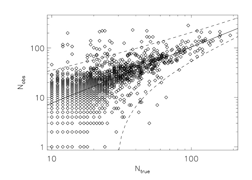
Figure 2.— The estimated probability matrix $\hat{P}(N_{obs}|N_{t})$ in Mock A. Non-zero matrix elements are marked with diamonds. The best-fit power law to the maximum-likelihood relation between $N_{obs}$ and $N_{t}$ is shown above as the thick solid line. The dashed curves define the signal band: everything within these lines is considered signal in the sense that it corresponds to proper halo-cluster matches. Points outside this band, including the points on each axis, are considered noise in the sense that they represent catastrophic errors of the cluster-finding algorithm (see text for how the dashed lines are defined); these points will contribute to the incompleteness and the impurity of the sample. Note that blending, that is, matching of low richness halos to high richness clusters, is clearly more of a problem than halo splitting (matching of high richness halos to low richness cluster), as argued in Koester et al. (2007a). We only show $N_{t}\geq 10$ as this corresponds to the resolution limit of the simulation.

The observed fraction $\hat{P}(N_{obs}|N_{t})$ of halos with $N_{t}$ galaxies that are matched to clusters with $N_{obs}$ galaxies is our estimator for the matrix element $P(N_{obs}|N_{t})$. Figure 2 shows the non-zero matrix elements of the estimated probability matrix. We can see that this plot has the generic behavior we expected from §2: the majority of the non-zero matrix elements populate a diagonal band, with a few outliers which arise due to catastrophic errors in the cluster finding algorithm. We split the matrix $P(N_{obs}|N_{t})$ into a signal and a noise component as follows: first, we find the maximum-likelihood relation between $N_{obs}$ and $N_{t}$, that is, we select the matrix elements that maximize $P(N_{obs}|N_{t})$ at fixed $N_{t}$, restricting ourselves to the region $N_{t}\geq 10$ as this corresponds to the resolution limit of the simulations (ie, some halos which would contribute to lower $N_{t}$ could be missed). The maximum-likelihood matrix elements are then fit with a line $\mu(N_{t})$ using robust linear fitting (Press et al. 1992). The best-fit line is characterized by the two parameters $B_{0}$ and $\beta$ defined via

$$\mu_{ML}(N_{t})=20\exp(B_{0})(N_{t}/20)^{\beta}.$$ (20)

We now make the ansatz that the variance will, at least roughly, scale with this maximum likelihood relation, which would be the case for a Poisson-like process. The signal band is then defined as all matrix elements $(N_{t},N_{obs})$ such that

$$N_{obs} \geq \mu_{ML}(N_{t})-5\sqrt{\mu_{ML}(N_{t})},\ \mbox{and}$$ (21)

$$N_{obs} \leq \mu_{ML}(N_{t})+10\sqrt{\mu_{ML}(N_{t})}$$ (22)

Non-signal halo-cluster pairs are defined to be noise. The signal/noise decomposition for Mock A can be seen in Figure 2: any matrix elements contained within the dashed lines are signal, and everything outside the dashed lines constitutes noise. The solid line going through the signal band is our best fit of the maximum-likelihood relation between $N_{obs}$ and $N_{t}$. Plots for the probability matrix for the other two mocks are qualitatively very similar.

While the above procedure is ad-hoc, we emphasize that we are defining the signal band. At the end of the day, it does not matter how we came up with the above definition, what matters is whether the definition is a useful one or not. For our purposes, we have simply selected a straightforward algorithm that qualitatively does what we need it to do, that is, cleanly separate signal points from catastrophic errors. Other algorithms would certainly be possible and equally valid, and there will undoubtedly be a definition that works best in the sense that that the statistical errors from a maximum likelihood analysis using the likelihood from §2 would be minimized. In this work, we simply wish to adopt a working definition, and we demonstrate below that even with this simplest definition where signal and noise are separated by eye, our model likelihood correctly describes the data and we can successfully recover the cosmological and bias parameters with exquisite precision.

3.5. Completeness

Having separated our halo-cluster pairs into a signal and a noise component, our estimator $\hat{c}(N_{t})$ for the completeness function is simply the fraction of halos with $N_{t}$ that are considered signal. In order to reduce the noise in these estimators, we also bin our halos into richness bins by demanding that each richness bin contain at least 50 halos. The resulting estimated completeness function in Mock A is shown in Figure 3 as the solid circles with error bars. Also shown in Figure 3 as triangles is the fraction of halos matched to cluster of any richness, regardless of whether the match constitutes signal or noise. We can see that for relatively rich systems with $N_{t}\gtrsim 25$, essentially all halos are detected, but completeness differs from unity due to some of these halos being blended. Conversely, at low richness, the vast majority of detected halos constitute signal, but the detected fraction decreases with decreasing richness, and as a result, the completeness function is essentially flat. We found this to be the case in each of the mocks.

We model the completeness function as a constant independent of richness. Our best-fit model for the completeness function is defined via $\chi^{2}$ minimization, and is seen in Figure 3 as a thick, solid line. Best fits for Mocks B and C are also shown as dashed and dotted lines respectively. Error bars for the $\chi^{2}$ minimization are assigned using the fact that the number of signal halos follows a binomial distribution with a detection probability $c(N_{t})$, from which we can compute the expected standard deviation of the ratio of signal halos to all halos in a given richness bin.

Figure 3.— The completeness function $c(N_{t})$ as measured in Mock A. Filled solid circles with error bars are the observed fraction of halos of richness $N_{t}$ matched within the signal band in Figure 2. For comparison, we also show the fraction of halos matched to clusters of any richness as triangles. The best fit completeness, modeled as constant, is shown as a solid line, and the grey regions represents the $95\%$ confidence interval in our completeness determination. Dashed and solid lines are obtained for Mocks B and C respectively, which are fully consistent with each other.

In order to determine whether our $\chi^{2}$ fit is a good fit, and to estimate the uncertainty in the best-fit completeness, we performed $10^{4}$ Monte Carlo realizations of our best-fit completeness model, and then treated these realizations in the same way we treated our data. We found the $\chi^{2}$ values measured in the mock to be consistent with our Monte Carlo $\chi^{2}$ distribution. The $95\%$ confidence interval for the completeness function in Mock A is shown in Figure 3 as a grey band. Each of the mocks have completeness measures that are consistent with each other.

3.6. Calibrating the Signal Matrix

Calibration of the signal matrix $P_{s}(N_{obs}|N_{t})$ is essentially a trial and error game since we have no a priori expectation for the form of $P_{s}(N_{obs}|N_{t})$. Note, however, that so long as we parameterize $P_{s}(N_{obs}|N_{t})$ in a way that is statistically consistent with the simulation constraints, it does not matter how we came up with our particular parameterization. Rather than discussing the various iterations we went through to find a successful model for $P_{s}(N_{obs}|N_{t})$, we have chosen to simply state our model, and then demonstrate that our parameterization is flexible enough to fully accommodate the simulation data. Our model for the probability matrix is

$$P_{s}(N_{obs}|N_{t})\propto\mbox{\rm erf}(x_{max})-\mbox{\rm erf}(x_{min})$$ (23)

where $x_{min}=(N_{obs}-\mu(N_{t})+1)/\sqrt{2\mbox{Var}(N_{t})}$, $x_{max}=(N_{obs}-\mu(N_{t})+2)/\sqrt{2\mbox{Var}(N_{t})}$, and

$$\mu(N_{t}) = 20\exp(B_{0}+0.14)(N_{t}/20)^{(\beta-0.12)}$$ (24)

$$\mbox{Var}(N_{obs}|N_{t}) = \exp(-3B_{0}+B_{1})\mu(N_{t}).$$ (25)

The factor of $20$ is simply our chosen pivot point. Note that $B_{0}$ and $\beta$ were defined earlier in equation 20, so that the only new parameter being introduced is $B_{1}$, which characterizes the variance of $P_{s}(N_{obs}|N_{t})$. The appearance of $-3B_{0}$ in the expression for Var$(N_{t})$ de-correlates $B_{0}$ and $B_{1}$, whereas the additive constants $0.14$ and $-0.12$ in the expressions for $\mu(N_{t})$ were empirically determined and characterize the difference between the mean value $\left\langle N_{obs}|N_{t}\right\rangle=\mu(N_{t})$ and the maximum likelihood value $\mu_{ML}(N_{t})$ from equation 20. Finally, the proportionality constant in equation 23 is set by demanding that the sum of all matrix elements over the signal band be equal to unity.

Figure 4.— $\chi^{2}$ distribution of $10^{4}$ Monte Carlo realizations of our best-fit model of the signal matrix $P_{s}(N_{obs}|N_{t})$ for Mock A. The $\chi^{2}$ value observed in the mock is marked by a thick, solid line at the bottom of the plot. We find that our model for $P_{s}(N_{obs}|N_{t})$ is indeed a good fit to the mock catalog data. This was the case for Mocks B and C as well.

We now demonstrate that this parameterization does indeed provide a good fit to the mock catalogs and estimate the uncertainties in our best fit parameters. To do so, we first find the best-fit value for $B_{1}$ by minimizing $\chi^{2}$ and assuming a binomial distribution for computing the error bars for each matrix element. We then compare the $\chi^{2}$ distributions obtained from $10^{4}$ Monte Carlo realizations of our best-fit model for each of our mocks to the $\chi^{2}$ value observed in the mocks directly. Figure 4 illustrates our result in the case of Mock A. It is clear from the figure that the model is indeed a good fit to the simulation data. This is true of Mocks B and C as well.

The top plot in Figure 5 shows the $95\%$ confidence regions of the parameters $B_{0}$ and $\beta$ in Mocks A, B, and C. The corresponding regions for the parameters $B_{0}$ and $B_{1}$ are shown in the bottom panel. It is evident that the best-fit parameters $B_{0}$ and $B_{1}$ in each mock are not fully consistent with each other, and that this variation represents a large systematic uncertainty in the probability matrix $P_{s}(N_{obs}|N_{t})$. Nevertheless, the slope $\beta$ appears to be robustly constrained, with roughly $\beta=1.18\pm 5\%\ (1\sigma)$. Early analysis of some recent simulations suggests that the scatter in $\beta$ is in fact larger than this, and the mean is somewhat lower, around $\beta\approx 1.1$, though a complete study of these simulations has not yet been completed. In what follows, we simply assume $\beta=1.18\pm 5\%$ unless noted otherwise, though we note we use a much more conservative prior $\beta=1.18\pm 15\%$ when analyzing the maxBCG cluster catalog constructed from SDSS data.

Figure 5.— $95\%$ confidence regions for the $B_{0}$ and $\beta$ parameters (top) and $B_{0}$ and $B_{1}$ (bottom) in each of our three mock catalogs. The dashed and solid contours are for Mocks A and B respectively. The shaded contours are $68\%$ and $95\%$ confidence regions in Mock A. The small filled circles mark the best-fit parameters from the mock catalogs, and were used to generate the Monte-Carlo realizations from which the confidence regions are derived. With the exception of $\beta$, the best-fit parameters in each of the mocks are clearly not consistent with each other, and represent a large systematic error. The solid line in the top panel corresponds to the value $\beta=1.18$, while the dashed lines mark the assumed 1$\sigma$ error $\Delta\beta/\beta=5\%$ in this work. The dotted lines in the top panel and the solid lines in the bottom panel mark the assumed $1\sigma$ region used in Rozo et al. (2007).

3.7. Purity

The purity function represents the fraction of clusters that are not well matched to a halo (i.e. that fall outside the signal band). Calibration of the purity function is thus completely analogous to the completeness function provided we switch the role of halos and clusters. That is, thinking of clusters as input and halos as output, we follow the exact same procedure we used to define the completeness function in order to define the purity function. Our estimate for of the purity function in Mock A is shown in Figure 6. Also shown as a solid line is our best-fit model, which we have chosen to parameterize as

$$p(N_{obs})=\exp(-x(N_{obs})^{2})$$ (26)

where

$$x(N_{obs})=p_{0}+p_{1}\left(\frac{\ln(15)}{\ln(N_{obs})}-1\right).$$ (27)

The factor of $\ln(15)$ is there simply to de-correlate $p_{0}$ and $p_{1}$. The best-fit models for Mocks B and C are also shown as dashed and dotted lines respectively. Finally, as with completeness, we generate $10^{4}$ Monte Carlo realizations to estimate the $95\%$ confidence regions of our best-fit parameters, and to test whether the model is a statistically acceptable fit to the data. We find that this is indeed the case, and the corresponding $95\%$ confidence band for Mock A is shown in Figure 6 as a grey band. The three mock catalogs are only marginally consistent with each other, but the purity is quite high in each of them.

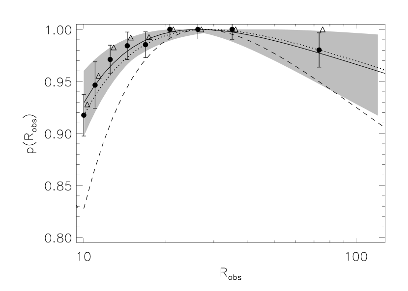
Figure 6.— Fraction of clusters matched to a halo within the signal band. Filled circles are the fraction measured in Mock A. The thick solid line is the best fit to the data, and the grey band represents the $95\%$ confidence band of the model. Dotted and dashed lines are the best fits for Mocks B and C respectively. For reference, we also show with triangles the fraction of clusters matched to halos of any richness.

3.8. Photometric Errors Calibration

We now calibrate the probability distribution $\rho(z_{c}|z_{h})$, that is, the distribution of photometric cluster redshift estimates in terms of the true halo cluster redshift. We characterize the photometric redshift distribution in terms of the redshift bias parameter $b=z_{c}/z_{h}$. The probability distribution $\rho_{b}(b|z_{h})$ is related to the probability distribution $\rho(z_{c}|z_{h})$ via

$$\rho(z_{c}|z_{h})=\frac{1}{z_{h}}\rho_{b}(b|z_{h}).$$ (28)

The advantage of working with $\rho_{b}(b)$ is that b correlates only very weakly with halo redshift $z_{h}$. Indeed, we found that the cross correlation coefficient between $b$ and $z_{h}$ in our mock catalogs was $\lesssim 0.1$. Moreover, we found the cross correlation between $b$ and $N_{obs}$ to be equally weak, so taking $\rho_{b}(b)$ to be richness independent is a good approximation for the maxBCG cluster catalog at richness $N_{obs}\geq 10$ (the richness range that will be used for cosmological constraints).

Figure 7 shows the distribution of bias parameters for each halo–cluster pair in Mock A. The distribution $\rho(b)$ is seen to be well fit by a Gaussian, and is thus completely characterized by the average bias parameter $\left\langle b\right\rangle$ and its standard deviation $\sigma_{b}$. The best-fit parameters for each of our mocks are $\left\langle b\right\rangle=1.00,1.02,$ and $1.03$ and $\sigma_{b}=0.04,0.03,$ and $0.05$ for Mocks A, B, and C respectively. These determinations have effectively zero statistical error; here again systematic variations from realization to realization represent our main source of uncertainty.

Figure 7.— Distribution of the photometric redshift bias parameter $b=z_{c}/z_{h}$ for Mock A. The distribution $\rho_{b}(b)$ is richness and redshift independent to a good approximation, and is well fit by a Gaussian, as shown above. The thick solid line at the bottom represent the best-fit value for the average bias.

4. Testing the Model

We now test whether our model can successfully reproduce the observed number counts in the mock catalogs. Even more importantly, we test whether we can successfully recover the cosmological and HOD parameters of the simulations with use of the likelihood function from §2. Throughout this section, we use the Jenkins et al. (2001) parameterization of the halo mass function. The linear power spectrum is computed using the low baryon transfer functions from Eisenstein & Hu (1999) with zero neutrino masses, and the initial power spectrum is assumed to be a Harrison-Zeldovich spectrum. Flatness is also assumed, and all cosmological parameters are held fixed except for $\sigma_{8}$, $\Omega_{m}$, and $h$. Allowing other parameters to vary should have only a minor impact on our results as it has been shown (White et al. 1993; Rozo et al. 2004) that local halo abundances are most sensitive to these three parameters.

4.1. Cluster Counts Comparison

We begin by comparing the cluster number counts in each of our three mocks to our model predictions using the simulation-calibrated values for all eight nuisance parameters (one completeness, two purity, two photo-$z$, and three signal matrix parameters). The input cosmology and HOD are taken directly from the mock catalog. There are, however, two important points concerning the mocks which we would like to highlight. First, the variance in the number of galaxies in halos of a given mass is somewhat larger than Poisson. Consequently, in this section we take $P(N_{t}|m)$ to be Gaussian, and calibrate the relation between $\mbox{Var}(N_{t}|m)$ and $\left\langle N_{t}|m\right\rangle$ directly from the mocks. Secondly, halo masses in the simulation were defined at an overdensity $\Delta=200$ with respect to critical, whereas our model requires masses to be measured at an overdensity of $200$ relative to the mean matter density. We transform the masses accordingly using the fitting functions from Hu & Kravtsov (2003). Our final uncertainty in the fitted values for the HOD is $\approx 3\%$ as estimated by examining the sensitivity of our best-fit parameters to the number of bins used for the calibration and the minimum mass cut considered when fitting the HOD. We will see below that this accuracy is comparable to the statistical uncertainty with which we can recover the best-constrained modes in parameter space.

Figure 8.— Comparison between the cluster counts measured in the mocks and our model predictions. Solid, dotted, and dashed curves represent Mocks A, B, and C. For clarity, we have also displaced mocks C and B to the right by a factor of $2$ and $4$ respectively. Error bars on the model values are obtained from the diagonal terms of the correlation matrix, and are roughly uncorrelated.

Figure 8 shows the cluster number counts in each of our three mock catalogs as well as our model predictions. The error bars associated with the model are simply the square root of the diagonal terms in the correlation matrix, and we have selected bins wide enough for the error bars to be roughly de-correlated. The agreement between the model predictions and the observed number counts in the mocks is excellent. Note that this agreement is not trivial. While it is true that our mass function is calibrated to the simulations, agreement between our prediction and the direct measurement in the mocks is only assured if our model successfully parameterizes the cluster-finding algorithm selection function. Figure 8 demonstrates that this is indeed the case, and that any systematics in the data have been properly taken into account.

4.2. Parameter Constraints for a Known Selection Function

We wish to test now whether we can successfully recover the cosmological and HOD parameters of the simulation with the use of the likelihood function constructed in §2. To do so, we use a Monte Carlo Markov Chain (MCMC) method to evaluate the likelihood function in parameter space and estimate the corresponding $68\%$ and $95\%$ confidence confidence contours of the likelihood function in parameter space. Details of our MCMC implementation, which draws heavily on the work by Dunkley et al. (2005), can be found in Appendix C. Throughout this paper, we consider cluster number counts binned in nine logarithmic bins between richness $N_{obs}=10$ and $N_{obs}=100$ within a single redshift slice ($[z_{min},z_{max}]=[0.12,0.25]$. We chose this binning as a compromise between having enough bins to accurately resolve the shape of the cluster richness function, while at the same time ensuring that every bin contained $\gtrsim 10$ clusters. This last property is desirable since the Gaussianity assumption of our likelihood function breaks down if the number of cluster within a given bin becomes too low.

We begin our analyzes by estimating the likelihood function while holding all of our nuisance parameters fixed to the simulation- calibrated values. That is, we assume we have perfect knowledge of the cluster selection function. This is useful for two reasons: first, it allows us to test whether our model likelihood successfully recovers the input cosmology and HOD parameters when the cluster selection function, that is, the probability matrix $P(N_{obs}|N_{t})$, is fully calibrated. In addition, investigating this case gives gives us a baseline for evaluating how well the signal matrix parameters must be calibrated before the quality of our parameter constraints decreases significantly. We should also note that, by and large, holding the cluster selection function fixed is a standard assumption in most analyses of cluster abundances. One of the most powerful features of our method is that, as we shall see in §4.3, it allows us to marginalize over uncertainties in the selection function.

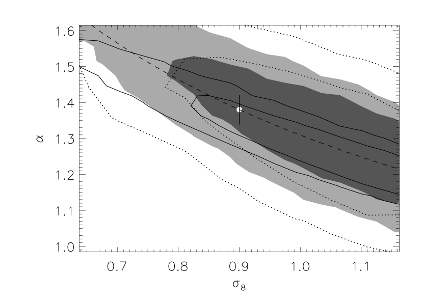
Figure 9.— Filled contours are the $68\%$ and $95\%$ confidence regions in the $\alpha-\sigma_{8}$ plane recovered for Mock A when holding all nuisance parameters fixed. The true parameters are marked as a small circle with error bars. We find that our likelihood model successfully recovers the simulation parameters to within the degeneracies intrinsic to the data. Also shown with solid curves are the $68\%$ and $96\%$ confidence regions obtained when using CMB and supernova like Gaussian priors $\Delta\Omega_{m}h^{2}=0.01$ and $\Delta h=0.05$. The dotted contours are obtained by marginalizing over all completeness, purity, and photo-$z$ parameters, and assuming $10\%$ priors on the signal matrix parameters (see §4.3 for discussion). The dashed line marks the expected degeneracy direction $\alpha^{2}\sigma_{8}=constant$, while the error bar centered on the true values of the simulation represents the $3\%$ error on $\alpha$ from the direct measurement of the HOD. Results for the three mocks considered were all very similar.

As expected, we find that there are strong degeneracies between between cosmology and HOD parameters. This is illustrated in Figure 9, where we plot the $68\%$ and $95\%$ confidence regions in the $\alpha-\sigma_{8}$ plane for Mock A. All three mocks give similar results. The degenerate parameter combination is roughly $\alpha^{2}\sigma_{8}=constant$, in agreement with the Fisher matrix estimate from Rozo et al. (2004). Also shown in this figure with a small circle with error bars are the known value of the parameters in the simulation; the error bars represent the $\approx 3\%$ uncertainty in our direct measurement of the HOD parameters. Clearly, to within the degeneracies intrinsic to the method, we successfully recover the input cosmology and HOD.

In light of the strong degeneracies inherent to the data, we focus now on the directions in parameter space that are best constrained by the data. These are defined by diagonalizing the parameter correlation matrix as estimated from the MCMC output. The best-constrained modes are those for which the eigenvalues are smallest. In the case of the Mock A, the top two normal modes are

$$x_{1} = \alpha^{0.97}\sigma_{8}^{0.92}(\Omega_{m}/M_{1})^{0.35}(\Omega_{m}M_{1})^{-0.06}h^{-0.45}$$ (29)

$$x_{2} = \alpha^{1.60}\sigma_{8}^{-0.26}(\Omega_{m}/M_{1})^{0.54}(\Omega_{m}M_{1})^{0.25}h^{0.12}.$$ (30)

Note the first parameter is essentially a cluster normalization condition, but with the Hubble and HOD parameters included. Moreover, it clearly reflects the expected $\Omega_{m}/M_{1}=constant$ degeneracy intrinsic to the halo mass function, though it is slightly modified due the weak sensitivity of the survey volume to $\Omega_{m}$. The second eigenvector does not have a simple interpretation (though see Appendix in Rozo et al. 2004). Hereafter, we refer to the top normal model in parameter space as the generalized cluster normalization condition.

We show the $68\%$ and $95\%$ confidence regions of these two parameters for Mock A in Figure 10. We find that not only do we indeed recover the correct simulation parameters, but that the associated statistical uncertainty is extremely small, of order $1\%$ and $4\%$ for the top two normal modes for our assumed survey of $1/8$ of the sky and redshift ranges $z\in[0.13,0.25]$. Given the small size of our error bars, the excellent agreement between our statistical analysis and the true simulation parameters is highly non-trivial. In particular, it explicitly demonstrates that if the selection function for the maxBCG catalog can be tightly constrained, optically-selected cluster samples can provide percent-level determinations of specific combinations of cosmological and HOD parameters.

Figure 10.— Filled contours are the $68\%$ and $95\%$ confidence regions in the $\alpha-\sigma_{8}$ plane for the the two best-constrained parameter combinations. The circle with error bars marks the input simulation parameters, and the error bars are a $3\%$ uncertainty from the the HOD fits to the simulation. Again, we find that our likelihood model successfully recovered the simulation parameters. Note that this is a very stringent test: the $1-\sigma$ error bars for these two top normal modes are $1\%$ and $5\%$ respectively. Also shown above with dotted curves are the $68\%$ and $95\%$ confidence regions obtained when using WMAP and supernova like Gaussian priors $\Delta\Omega_{h}^{2}=0.01$ and $\Delta h=0.05$. The apparent increase in the confidence regions is due to a slight rotation of the likelihood function in parameter space due to the introduction these cosmological priors.

It is also worth investigating to what extent our constraints can be improved upon through the use of other cosmological probes. In particular, the CMB places strong constraints on $\Omega_{m}h^{2}$ (see e.g. Hu et al. 1997; Hu & Dodelson 2002; Dodelson 2003), while supernovae data puts strong constraints on the value of the Hubble parameter $h$ (see e.g. Freedman et al. 2001). The reason these two particular priors are interesting is that their values have minimal or no dependence on the dynamical nature of dark energy. That is, these constraints do not depend on whether dark energy is a cosmological constant or not. Consequently, employing these priors still allows us to use cluster abundances for studying the dark energy. Note that this is not the case for all priors. For instance, the CMB data can also provide priors on $\sigma_{8}$, provided the power spectrum at last scattering is extrapolated to the present epoch using a $\Lambda\mbox{CDM}$ cosmology. Clearly, such a prior is useless if one is interested in constraining the behavior of the dark energy. Indeed, this is precisely why estimating $\sigma_{8}$ is an interesting problem: deviations from the CMB interpolated value for $\sigma_{8}$ could signal a failure of the $\Lambda$CDM model.

To investigate the impact that CMB and supernova like priors can have on our results, we repeat the above analysis, but including now Gaussian priors of width $\Delta\Omega_{m}h^{2}=0.01$ and $\Delta h=0.05$ centered on the simulation cosmology. The width of these priors is set by the current uncertainty in each of the two cosmological parameters as constrained by the CMB and supernovae respectively (Spergel et al. 2006). We find that including these cosmological priors has minimal impact on how well our normal modes are constrained. This is shown in Figure 9, where we find that the $\alpha_{N}-\sigma_{8}$ degeneracy is only marginally reduced. Even more telling is Figure 10, where we show the confidence regions of the normal modes found in the no priors case. Note that the confidence regions slightly increase rather than decrease due to the rotation of the likelihood function in parameter space due to the introduction of the priors. Indeed, we find that including priors in our analysis results in not just two but three highly constrained modes at roughly $1\%$, $2\%$, and $5\%$ accuracy. The first and the third are almost identical to the normal modes found in the no priors case, and the ones shown in Figure 10. The second normal mode, on the other hand, is largely parallel to the direction of our priors.

In summary, we have found that local cluster abundances estimated from large surveys can provide percent-level constraints on combinations of cosmological and HOD parameters if the selection function, i.e. completeness, purity, and the signal matrix, is known precisely. Individual parameters cannot be constrained due to intrinsic degeneracies in the data. Finally, adding cosmological priors from CMB and/or supernovae has minimal impact on the best-constrained parameter combinations.

4.3. Marginalizing Parameter Constraints Over Uncertainties in the Selection Function

Consider now marginalization over uncertainties in the selection function. We found that the completeness, purity, and photometric redshift error parameters were well constrained from the simulations, and varying them through the range of values measured from the simulations had minimal impact on the estimated number counts. Indeed, upon adopting top hat priors corresponding to the $95\%$ regions of these parameters we find that our results are largely identical to the ones presented in §4.2. Consequently, henceforth every result we present is marginalized over the completeness, purity, and photo-$z$ parameters.

The signal matrix parameters, on the other hand, are a different story. We saw in §3.6 that the slope $\beta$ of the mean relation between $N_{t}$ and $N_{obs}$ was relatively well constrained, and that a Gaussian prior on $\beta$ of the form $\beta=1.18\pm 5\%$ appears reasonable based on this set of simulations. Consequently, unless specially stated otherwise, we shall assume this prior in all of our analysis. We also saw, however, that the amplitudes $B_{0}$ and $B_{1}$ of the signal matrix had large systematic errors. In fact, these errors are large enough that attempts to constrain cosmology and HOD in the simulations using priors that covered the whole range of selection functions observed in the simulations proved unsuccessful. We have thus chosen to investigate how more moderate uncertainties in the amplitudes affect our results, with an eye towards future work which may improve our understanding of the cluster selection function. To do so, we ran MCMCs with $5\%$, $10\%$, $15\%$, and $20\%$ priors on the signal matrix parameters $B_{0}$ and $B_{1}$ using the observed number counts in Mock A. Due to the computational effort involved in running MCMCs for each model we consider, we focus on Mock A only. There is no particular reason why this realization was chosen over the other two, and, based on our results from the previous section, we have no reason to suspect that any one realization would lead to substantially different results than the other two.

Because of the large degeneracies in parameter space, we have chosen to focus on the two best-constrained modes in parameter space to quantify the sensitivity of our results to uncertainties in the values of $B_{0}$ and $B_{1}$. We find that the best-constrained normal mode is robust to $\approx 15\%$ uncertainties in the selection function. In particular, the direction of the mode remains constant, and the uncertainty in the parameter increases linearly with the width of the assumed priors, as illustrated in Figure 11. By $20\%$ uncertainties in the amplitudes $B_{0}$ and $B_{1}$, however, the top mode has rotated away slightly, and its uncertainty starts growing faster than linearly with the width of the amplitude priors. Nevertheless, it is remarkable that even with uncertainties as large as $20\%$ in the cluster selection function we can recover the top normal mode in parameter space to better than $5\%$ accuracy.

Figure 11.— Sensitivity of the error of the best-constrained normal mode in parameter space to uncertainties in the cluster selection function. This mode corresponds to a generalized cluster normalization condition, and both its amplitude and direction are fairly robust for up to $\approx 15\%$ uncertainties in the cluster selection function, characterized in this case by the amplitudes $B_{0}$ and $B_{1}$ (see §3.6). Filled circles assume a $5\%$ prior on the slope $\beta$, while the triangle is obtained assuming a $10\%$ prior on $\beta$. Finally, the square marks the error on the generalized cluster normalization condition when including CMB and supernova like priors on $\Omega_{m}h^{2}$ and $h$ (compare to Figure 9. The slight increase in the uncertainty is due to the change in orientation of the likelihood function.

To investigate how sensitive our results were to our assumptions about $\beta$, we also considered the case in which all signal matrix parameters (including the slope $\beta$) were known to $10\%$ accuracy. The corresponding error on the top normal mode for this case is shown in Figure 11 as a triangle, and demonstrates that there is little loss of information by the additional uncertainty in $\beta$. It is worth noting that the two model parameters that are most closely aligned with the top normal mode are $\alpha$ and $\sigma_{8}$. Consequently, constraints in the $\alpha-\sigma_{8}$ are relatively robust to uncertainties in the signal matrix, as shown in Figure 9.

We now turn our attention to the behavior of the second best-constrained mode, which we find is not stable to uncertainties in the signal matrix. Specifically, we find that there is a factor of two increase in the error of this mode in going from fixed nuisance parameters to $5\%$ uncertainties in the signal matrix. Moreover, the direction of the second best-constrained normal mode is substantially different between the two cases. Curiously, as we increased the width of our prior on the amplitudes $B_{0}$ and $B_{1}$, we found that the second best-constrained mode remained relatively constant both in direction and width, suggesting the large difference between the fixed nuisance parameter case and the $5\%$ priors case was driven largely by the uncertainties in the slope $\beta$. We tested this scenario by running an additional chain with $10\%$ priors on all signal matrix parameters, and found that, indeed, with the new priors for $\beta$ the second best-constrained mode was severely affected, both in terms of the direction and the percent-level accuracy with which it could be recovered. We conclude that there is a large degeneracy between cosmological and HOD parameters and the slope $\beta$. This is an important, though rather unfortunate, result, as it implies that to fully recover the constraining power of large local cluster samples, the slope of the relation between $N_{obs}$ and $N_{t}$ must be known to high accuracy.

In light of these results, it is worth returning to the question of whether or not CMB and supernova priors on cosmological parameters could substantially alter our conclusions. To test this, we ran an addition MCMC using CMB and supernova like Gaussian priors $\Delta\Omega_{m}h^{2}=0.01$ and $\Delta h=0.05$, assuming $15\%$ uncertainties in $B_{0}$ and $B_{1}$, and our default $5\%$ level uncertainty in $\beta$. We mark the corresponding uncertainty on the cluster normalization condition in Figure 11 as a square. Note that the error on the cluster normalization condition slightly increases upon inclusion of the prior. This is again indicative of an overall distortion of the orientation of the likelihood surface in parameter space upon inclusion of the priors. Indeed, upon including the priors, we found that the best-constrained mode was no longer the cluster normalization condition, but rather falls close to the direction of the assumed priors. The generalized cluster normalization condition then becomes the second best-constrained eigenmode, and was itself slightly rotated relative to the fixed nuisance parameters case. The next best-constrained eigenmode was found to be unstable to the introduction of cosmological priors.

5. Summary and Discussion

In this work we have introduced a general framework for characterizing the selection function of optical cluster finding algorithms. The fundamental assumption in our method is that the scatter in the mass-observable relation for a cluster finding algorithm can be split into an intrinsic scatter, and an observable scatter due to the imperfection of the cluster finding algorithm. We show that the inability to fully characterize catastrophic errors in richness assignments naturally gives rise to the concepts of purity and completeness in quantitative form. These definitions of purity and completeness are well defined and are particularly well suited to cosmological abundance analyses.

This method could potentially be applied to characterizing the selection function and to cosmological parameter estimation for a wide range of current and future cluster samples. Here, we have demonstrated its utility by application to the maxBCG cluster finding algorithm (Koester et al. 2007a), run on mock galaxy catalogs produced using three different realizations of the ADDGALS prescription for connecting a realistic galaxy population to large dissipationless simulations, of comparable volume to the SDSS data sample (detailed in Wechsler et al. 2007). In a companion paper (Rozo et al. 2007), we apply this method to the SDSS maxBCG cluster catalog (Koester et al. 2007b).

By matching the input halos to the detected clusters, we have quantitatively calibrated the maxBCG selection function in each of the three mock catalogs, and demonstrated that with knowledge of this selection function we can accurately recover the underlying cosmology and HOD parameters of the simulations to within the intrinsic degeneracies of the data. Moreover, we have shown that this is still the case when the selection function is only known to $\approx 15\%$ accuracy, though the uncertainty in the recovered parameters starts growing quickly after that.

We conclude that it is possible to provide tight cosmological and HOD constraints using optically-selected cluster catalogs, but doing so requires a better constrained cluster selection function that we currently have. This is an important and non-trivial result: it explicitly shows that the popular view that projection effects present an insurmountable obstacle for precision cosmology with with optically-selected cluster catalogs is no longer the case. We have demonstrated that the maxBCG cluster catalog is highly complete and pure, and, more importantly, that any such effects can be incorporated into our cosmological parameter analysis through a detailed calibration of the cluster selection function. Provided the selection function is known with relative accuracy, optical cluster catalogs can be useful tools for precision cosmology.

In the present work, we have not made an exhaustive attempt to characterize the uncertainties in the cluster selection function. Here, we investigated three realizations of the empirically-motivated galaxy biasing scheme ADDGALS, applied to one cosmological model, the large, low resolution Hubble Volume simulation. Although all three realizations provide a reasonable representation of galaxies in the local Universe, including realistic luminosity and color evolution and clustering properties, and a red sequence population that is a good match to maxBCG, the three simulations had different HOD descriptions. Our results suggest that the cluster selection function depends to some extent on the specific HOD of the simulation, at least for the richness measurements we considered. To mitigate this uncertainty in our analysis of the maxBCG data, in Rozo et al. (2007), we perform the analysis assuming only that the shape of the selection function is the same in both the simulations and the data, and greatly relaxing the prior on the slope $\beta$ relating the mean observed and intrinsic richness.

We end now by considering the obvious question: can this situation improve? We remain optimistic that future work will allow tighter and more robust constraints on the maxBCG selection function than are presented here, which will allow us to maximize the power of the large maxBCG data set. We are proceeding along three fronts:

• Improved richness definitions. A robust calibration for $P(N_{obs}|N_{t})$ for arbitrary definitions of $N_{t}$ and $N_{obs}$ may indeed be hard to come by, it is entirely plausible that we can refine our definitions of halo and cluster richness to considerably improve our understanding of the selection function. For instance, in this work, no attempt was made to make $N_{obs}$ an unbiased estimator of $N_{t}$, so something as simple as including a color cut in our definition of $N_{t}$ could significantly improve our model. If one can define $N_{obs}$ such that, by construction, $\left\langle N_{obs}|N_{t}\right\rangle=N_{t}$, not only will the number of nuisance parameters immediately go down by two, but also some of the large degeneracies we uncovered in this work will become irrelevant.

• A detailed characterization of the variance between a range of models. A crucial question is whether the selection function calibration is robust to changes not only in the halo occupation of the galaxies but also in the cosmological parameters of the underlying simulation. Although we didn’t explore this directly in the mocks investigated here, we were generous in the range of galaxy populations applied to the simulations. Scatter between selection function parameters will likely go down if we apply further observational constraints on the galaxy populations. We then intend a wide exploration of parameter space after these constraints have been applied.

• The addition of mass calibration data from maxBCG itself. Information on the mass scale is directly available from both stacked lensing measurements (Sheldon et al. 2007, Johnston et al, in preparation), stacked X-ray measurements (Rykoff et al. 2007), and from the velocity dispersions of the galaxies in clusters (Becker et al. 2007). These data provide substantial additional constraints on combinations of our selection function parameters, and will allow us to use weaker priors in both the selection function and cosmological parameter space.

Appendix A Summary of Equations

For reference, we summarize below all the formulae that quantitatively describe our model. Let $\mathbf{N}=\{N_{1},...,N_{M}\}$ be the number of clusters in richness bins $1$ through $M$, and $\mathbf{p}$ be the parameters characterizing cosmology, HOD, purity, completeness, and the signal matrix $P_{s}(N_{obs}|N_{t})$. The likelihood function ${\cal{L}}(\mathbf{p}|\mathbf{N})$ is given by

$${\cal{L}}(\mathbf{p}|\mathbf{N})\propto\frac{1}{\sqrt{(2\pi)^{M}\mbox{det}(C)}}\exp\left\{-\frac{1}{2}(\mathbf{N}-\left\langle\mathbf{N}\right\rangle)\cdot C^{-1}\cdot(\mathbf{N}-\left\langle\mathbf{N}\right\rangle)\right\}.$$ (A1)

Above, $\left\langle\mathbf{N}\right\rangle$ is the expectation value for the data vector, and $C$ is the correlation matrix of the observables. The number of clusters in a given richness bin $a$ is given by

$$\left\langle N_{a}\right\rangle=\int dz_{h}d^{2}\hat{\mathbf{n}}_{h}\ \chi^{2}\frac{d\chi}{dz_{h}}\left\langle{\rm NewA}\right\rangle\left\langle\varphi|z_{h}\right\rangle\left\langle\Theta|\hat{\mathbf{n}}_{h}\right\rangle$$ (A2)

where $\chi$ is the comoving distance to redshift $z_{h}$. The function $\left\langle\varphi|z_{h}\right\rangle$ is the effective redshift selection function of the survey, and is given by

$$\left\langle\varphi|z_{h}\right\rangle=\int dz_{c}\ \rho(z_{c}|z_{h})\varphi(z_{c})$$ (A3)

where $\varphi(z_{c})=1$ if the photometric cluster redshift $z_{c}\in[z_{min},z_{max}]$ and $\varphi(z_{c})=0$ otherwise, and $z_{min}$ and $z_{max}$ define the redshift selection criteria for the survey. Likewise, the function $\left\langle\Theta|\hat{\mathbf{n}}_{h}\right\rangle$ is the effective angular mask of the survey, and is given by

$$\left\langle\Theta|\hat{\mathbf{n}}_{h}\right\rangle\int d^{2}\hat{\mathbf{n}}_{c}\Theta(\hat{\mathbf{n}}_{c})\rho(\hat{\mathbf{n}}_{c}|\hat{\mathbf{n}}_{h})$$ (A4)

where $\Theta(\hat{\mathbf{n}}_{c})$ is the angular mask of the survey. In this work, we have assumed $\rho(\hat{\mathbf{n}}_{c}|\hat{\mathbf{n}}_{h})=\delta(\hat{\mathbf{n}}_{c}-\hat{\mathbf{n}}_{h})$. Finally, $\left\langle{\rm NewA}\right\rangle$ is the expected comoving cluster number density as a function of redshift, and is given by

$$\left\langle n_{a}\right\rangle=\int dm\frac{d\langle\bar{n}\rangle}{dm}\left\langle c\psi_{a}/p|m\right\rangle.$$ (A5)

where $\left\langle dn/dm\right\rangle$ is the halo mass function, and the quantity $\left\langle c\psi_{a}/p|m\right\rangle$ represents the mass binning of the survey, given by

$$\left\langle c\psi_{a}/p|m\right\rangle=\sum_{N_{t}}c(N_{t})\tilde{\psi}_{a}(N_{t})P(N_{t}|m).$$ (A6)

where $c(N_{t})$ is the completeness function, and $P(N_{t}|m)$ is the HOD. $\tilde{\psi}_{a}$ is the binning function in terms of $N_{t}$, which is related to the top hat richness binning function $\psi_{a}(N_{obs})$ via

$$\tilde{\psi}_{a}(N_{t})=\sum_{N_{obs}}\frac{\psi_{a}(N_{obs})}{p(N_{obs})}P_{s}(N_{obs}|N_{t}).$$ (A7)

where the sum is over all $N_{obs}$ values within the signal band, $p(N_{obs})$ is the purity function, and $P_{s}(N_{obs}|N_{t})$ is the signal matrix.

We also summarize below the equations describing the correlation matrix $C$. In particular, the Poisson contribution to the correlation matrix takes on the form

$$(C_{a,a^{\prime}})_{P}=\delta_{a,a^{\prime}}\int(\chi^{2}\frac{d\chi}{dz_{h}}dz_{h}d\hat{\mathbf{n}}_{h})\int dm\frac{d\langle\bar{n}\rangle}{dm}\left\langle c\psi_{a}/p^{2}|m\right\rangle\left\langle\Theta|\hat{\mathbf{n}}_{h}\right\rangle\left\langle\varphi|z_{h}\right\rangle.$$ (A8)

Note that, schematically, this contribution takes on the form $C_{a,a^{\prime}}\approx\delta_{a,a^{\prime}}\left\langle N_{a}\right\rangle/p$. This is exactly what we would expect: if $N$ is the number of observed clusters and $N_{s}$ the number of signal clusters, then $N=N_{s}/p$, so $\mbox{Var}(N)=\mbox{Var}(N_{s})/p^{2}=N/p$. To this Poisson contribution we must also add the sample variance term

$$(C_{a,a^{\prime}})_{S}=\left\langle bGN_{a}\right\rangle\left\langle bGN_{a^{\prime}}\right\rangle\sigma^{2}(V)$$ (A9)

where

$$\left\langle bGN_{a}\right\rangle=V\left[\int dm\ b(m)\frac{d\langle\bar{n}\rangle}{dm}\left\langle c\psi_{a}/p|m\right\rangle G\right]_{\bar{z}},$$ (A10)

$V$ is the survey volume, and $\sigma^{2}(V)$ is the rms variance of the linear density field over the sample volume probed. An additional contribution to the correlation matrix arises from the stochasticity of the mass-richness relation, which leads to uncertainties in the precise mass binning of the cluster sample. This contribution takes on the form

$$(C_{a,a^{\prime}})_{B} = \int dz_{h}d^{2}\hat{\mathbf{n}}_{h}\ \chi^{2}\frac{d\chi}{dz_{h}}\left\langle\varphi|z_{h}\right\rangle\left\langle\Theta|\hat{\mathbf{n}}_{h}\right\rangle\left\langle\varphi|z_{h}\right\rangle$$ (A12)

$$\times\int dm\ \frac{d\langle\bar{n}\rangle}{dm}\left[\delta_{a,a^{\prime}}\left\langle c\psi_{a}/p^{2}|m\right\rangle-\left\langle c\psi_{a}/p|m\right\rangle\left\langle c\psi_{a^{\prime}}/p|m\right\rangle\right].$$

Note that in the above expression it is evident that neighboring bins are always negatively correlated, reflecting the fact that halos scattering into a given bin $a$ must have scattered out of some other bin $a^{\prime}$. Also, there is an additional contribution to do photometric redshift uncertainties, which reduces to

$$(C_{a,a^{\prime}})_{Z}=\delta_{a,a^{\prime}}\int dz_{h}d^{2}\hat{\mathbf{n}}_{h}\ \chi^{2}\frac{d\chi}{dz_{h}}\left\langle\Theta|\hat{\mathbf{n}}_{h}\right\rangle\left[\left\langle\varphi|z_{h}\right\rangle-\left\langle\varphi|z_{h}\right\rangle^{2}\right]\int dm\ \frac{d\langle\bar{n}\rangle}{dm}\left\langle c\psi_{a}/p^{2}|m\right\rangle.$$ (A13)

Finally, there are uncertainties due to the stochastic nature of the purity function, which take on the form

$$(C_{a,a^{\prime}})_{p}=\delta_{a,a^{\prime}}\int dz_{h}\frac{dV}{dz_{h}}\left\langle\varphi|z\right\rangle\int dm\frac{d\langle\bar{n}\rangle}{dm}\left\langle c\psi_{a}(1-p)/p|m\right\rangle.$$ (A14)

Note that when the purity is exactly equal to one, the purity contribution to the correlation matrix vanishes, as it should.

Appendix B Matching Algorithms Considered in this Work

The type of membership matching algorithms we considered can be broadly grouped into one of two categories: deterministic matching algorithms and probabilistic matching algorithms. We considered four deterministic matching algorithms:

1. Maximum shared membership matching: Each halo is matched to the cluster containing the largest number of galaxies belonging to the halo.

2. BCG matching: A halo is matched to the cluster containing the halo’s BCG.

3. Exclusive maximum shared membership matching: Halos are first rank ordered according to their richness $N_{t}$. Starting with the richest halo, its cluster match is found through maximum shared membership matching. The matched cluster is then removed from the list of candidate matches for all other halos, and the procedure is iterated.

4. Exclusive BCG matching: This is exactly analogous to exclusive maximum shared membership, only BCG matching is used to match halos to clusters at each step.

In addition to these four matchings, we considered what we have called probabilistic matching schemes, which are essentially generalizations of the deterministic matching schemes. The idea is as follows: imagine listing all halos and all clusters in a two column format, so that the left column contains all halos and the right column contains all clusters. Pick a cluster $\alpha$, and draw a line connecting halo $\alpha$ to all clusters $\beta$ which share members with halo $\alpha$. Let then $f_{\alpha\beta}$ be the fraction of galaxies in halo $\alpha$ contained in cluster $\beta$. Maximum shared membership matching consists of selecting the cluster $\beta$ which maximizes $f_{\alpha\beta}$ with probability one. More generally, however, one could imagine replacing this probability with some other probability function $p(f_{\alpha\beta})$, an obvious choice being $p(f_{\alpha\beta})=f_{\alpha\beta}$ which we refer to as proportional random matching. Another possible choice is random membership matching, where we set $p(f_{\alpha\beta})=1/N_{\alpha}$ where $N_{\alpha}$ if the total number of candidate cluster matches for halo $\alpha$.

Consider now the probability matrix $P(N_{obs}|N_{t})$ in the case of probabilistic matching. One has that

$$P(N_{obs}|N_{t})=\sum_{\alpha}P(N_{obs}|\alpha)P(\alpha|N_{t})$$ (B1)

where $P(N_{obs}|\alpha)$ is the probability that halo $\alpha$ be matched to a cluster with $N_{obs}$ galaxies, and $P(\alpha|N_{t})=\delta_{N_{\alpha,N_{t}}}/N(N_{t})$ is the probability of picking halo $\alpha$ at random from a the set of $N(N_{t})$ halos of richness $N_{t}$. All that remains is computing the probability $P(N_{obs}|\alpha)$, which is simply given by

$$P(N_{obs}|\alpha)=\sum_{\beta}\delta_{R_{\beta},N_{obs}}p(f_{\alpha\beta}).$$ (B2)

Putting it altogether we find

$$P(N_{obs}|N_{t})=\frac{1}{N(N_{t})}\sum_{\alpha,\beta}\delta_{R_{\alpha},N_{t}}\delta_{R_{\beta},N_{obs}}p(f_{\alpha\beta}).$$ (B3)

Figure 1 plots the cost function $\Delta(N_{obs})$ for each of the two exclusive matching algorithms, and for the non-exclusive maximum shared membership matching in the case of the s simulation. The corresponding plots for the other simulations are quite similar. The non-exclusive BCG matching and the probabilistic matchings give results almost identical to the non-exclusive maximum shared membership matching case, and are very much worse than any of the exclusive matching algorithms, demonstrating that enforcing a one to one matching between halos and clusters is of paramount importance. It is worth noting that maxBCG does not enforce exclusive galaxy membership for cluster, that is, a galaxy can be a member of more than one cluster.

We focus now on the exclusive matching algorithms. In particular, each of these algorithms has an upturn in the cost function at high richness. This upturn is due to what we called noise in §2, i.e. catastrophic errors in the cluster-finding algorithm. These catastrophic errors are in reality quite rare, so the mixing induced by non-zero matrix elements due to catastrophic errors generate an unrealistically large amount of mixing between low richness halos and high richness clusters. Consequently, we believe the upturn at high richness is unphysical. Given this assumption, based on Figure 1 we chose exclusive maximum shared membership matching as our fiducial halo-cluster matching algorithm for the remainder of this work.

Appendix C MCMC Implementation

Evaluation of the likelihood function in a multi-dimensional parameter space can be extremely time consuming. Fortunately, not all of parameter space needs to be sampled, only the high likelihood regions. We achieve this through the use of Monte Carlo Markov Chains (MCMC), drawing heavily on the work by Dunkley et al. (2005) (for some introductory material on MCMC methods see e.g. Wasserman 2004).

In this work, we require not only to find the point of maximum likelihood, but also the $68\%$ and $95\%$ probability likelihood contours. Dunkley et al. (2005) showed that the number of points $N$ in a chain necessary to recover a $p$ confidence region with accuracy $q$ is $N\approx 3.3D/q^{2}/(1-p)$ where $D$ is the dimensionality of the parameter space. When we hold our nuisance parameters fixed to the simulation calibrated values, the total number of free parameters is five, so the number of points in the chain necessary to recover the $95\%$ confidence regions with $10\%$ accuracy is $N\approx 3\cdot 10^{4}$. We choose $N=5\cdot 10^{4}$ steps as the default length of our chains in this case. When fitting for all 13 parameters (cosmology+HOD+nuisance), the expected minimum number of points required to appropriately sample the likelihood function is thus $N\approx 10^{5}$, which we adopt as our default length for the chains.

Now, in order to achieve convergence quickly, some take must be taken to ensure that the chain is close to optimal. In particular, both the direction and size of the steps in the MCMC need to be carefully chosen. Here, we follow Dunkley et al. (2005), and take random steps along the principal components of the parameter correlation matrix. For each normal mode, we chose a step size $2\sigma/\sqrt{D}$ where $\sigma$ is the eigenvalue of the principal component and $D$ is the number of parameters (either $4$ or $\approx 10$ in our case). This step size is slightly smaller than the value reported in Dunkley et al. (2005), and is chosen because, as shown by Dunkley et al. (2005), for problems with a large number of parameters, it is in general better to err on the low side when estimating the optimal step size.

Finally, in order to be able to take steps along the principal components of the correlation matrix, we must first estimate the correlation matrix. To do so, we follow an iterative procedure where we start our MCMC in a region of relatively high likelihood, and use the first $1000$ steps to estimate the correlation matrix varying only cosmological and HOD parameters to resolve any intrinsic degeneracies of the model. For the next $2000$ steps we introduce the parameters characterizing the signal matrix as additional degrees of freedom, and estimate the new correlation matrix. We then allow the completeness, purity, and photo-$z$’s parameters to vary, and use $3000$ steps to estimate the correlation matrix. We make one final iteration of $4000$ steps and re-estimate the correlations matrix, which is used to take an additional $10^{5}$ steps which constitute our chain for the purposes of parameter estimation. When keeping nuisance parameters fixed, we use only two training runs to estimate the correlation matrix, the first with $1000$ steps, and then an iteration with $2000$ steps. We checked all our chains for convergence with the tests described in Dunkley et al. (2005).

We found that letting the signal matrix parameters float in our MCMCs introduced a very serious numerical difficulty. In particular, we found that in our model there was a small region of the $13$ dimensional space where the estimated correlation matrix of the cluster number counts becomes singular, causing the likelihood function to blow up. We found this difficulty arose due to detailed numerical cancellation between the Poisson and binning contributions to the correlation matrix. Consequently, we decided to approximate the correlation matrix by replacing the Poisson contribution estimated from our model by $1/N_{a}$ where $N_{a}$ are the observed number counts. In high likelihood regions, one has $\left\langle N_{a}\right\rangle\approx N_{a}$ and hence the approximation should be valid. Indeed, we explicitly checked that we could reproduce all of our results when keeping the signal matrix parameters fixed while employing this approximation.

The end result of our approximation was to greatly reduce the volume of parameter space where the cluster counts correlation matrix became singular. A typical output from a chain computed with the above likelihood is shown in Figure 12. The fact the singular region in parameter space is small can be seen from the fact that the chain ran for $\approx 9\cdot 10^{4}$ steps before encountering the singularity. Moreover, once the chain stepped into this region, it froze, demonstrating that virtually every step took it outside the singularity. To avoid this behavior, we can simply carve out the singular region of parameter space, which we do by introducing a cut on the likelihood. In particular, we set ${\cal{L}}=0$ for any region where our model results in an unrealistically large likelihoods. It is worth noting that introducing such a cut without affecting the performance of the chain is not difficult. For instance, in Figure 12, we see that the likelihood ratio between the singular region and the physical region is $\approx 10^{65}$.

Figure 12.— An MCMC output illustrating the singularity of the correlation matrix in a small region of parameter space. If the estimated correlation matrix of the cluster number counts becomes singular, the likelihood function is infinite. To avoid the corresponding small problem region in parameter space we introduce a likelihood cut. See text for more discussion.

References

- Abell (1958) Abell, G. O. 1958, ApJS, 3, 211
- Abell et al. (1989) Abell, G. O., Corwin, Jr., H. G., & Olowin, R. P. 1989, ApJS, 70, 1
- Becker et al. (2007) Becker, M. et al. 2007, in preparation.
- Berlind et al. (2006) Berlind, A. A. et al. 2006, ApJS, 167, 1
- Blanton et al. (2003) Blanton, M. R., Hogg, D. W., Bahcall, N. A., Brinkmann, J., Britton, M., Connolly, A. J., Csabai, I., Fukugita, M., Loveday, J., Meiksin, A., Munn, J. A., Nichol, R. C., Okamura, S., Quinn, T., Schneider, D. P., Shimasaku, K., Strauss, M. A., Tegmark, M., Vogeley, M. S., & Weinberg, D. H. 2003, ApJ, 592, 819
- Bond et al. (1991) Bond, J. R., Cole, S., Efstathiou, G., & Kaiser, N. 1991, ApJ, 379, 440
- Dalton et al. (1997) Dalton, G. B., Maddox, S. J., Sutherland, W. J., & Efstathiou, G. 1997, MNRAS, 289, 263
- Dodelson (2003) Dodelson, S. 2003, Modern cosmology (Modern cosmology / Scott Dodelson. Amsterdam (Netherlands): Academic Press. ISBN 0-12-219141-2, 2003, XIII + 440 p.)
- Dunkley et al. (2005) Dunkley, J., Bucher, M., Ferreira, P. G., Moodley, K., & Skordis, C. 2005, MNRAS, 356, 925
- Eisenstein & Hu (1999) Eisenstein, D. J. & Hu, W. 1999, ApJ, 511, 5
- Eke et al. (2004) Eke, V. R., Baugh, C. M., Cole, S., Frenk, C. S., Norberg, P., Peacock, J. A., Baldry, I. K., Bland-Hawthorn, J., Bridges, T., Cannon, R., Colless, M., Collins, C., Couch, W., Dalton, G., de Propris, R., Driver, S. P., Efstathiou, G., Ellis, R. S., Glazebrook, K., Jackson, C., Lahav, O., Lewis, I., Lumsden, S., Maddox, S., Madgwick, D., Peterson, B. A., Sutherland, W., & Taylor, K. 2004, MNRAS, 348, 866
- Evrard et al. (2002) Evrard, A. E., MacFarland, T. J., Couchman, H. M. P., Colberg, J. M., Yoshida, N., White, S. D. M., Jenkins, A., Frenk, C. S., Pearce, F. R., Peacock, J. A., & Thomas, P. A. 2002, ApJ, 573, 7
- Freedman et al. (2001) Freedman, W. L., Madore, B. F., Gibson, B. K., Ferrarese, L., Kelson, D. D., Sakai, S., Mould, J. R., Kennicutt, Jr., R. C., Ford, H. C., Graham, J. A., Huchra, J. P., Hughes, S. M. G., Illingworth, G. D., Macri, L. M., & Stetson, P. B. 2001, ApJ, 553, 47
- Gal et al. (2003) Gal, R. R., de Carvalho, R. R., Lopes, P. A. A., Djorgovski, S. G., Brunner, R. J., Mahabal, A., & Odewahn, S. C. 2003, AJ, 125, 2064
- Gal et al. (2000) Gal, R. R., de Carvalho, R. R., Odewahn, S. C., Djorgovski, S. G., & Lopes, P. A. 2000, Bulletin of the American Astronomical Society, 32, 1581
- Gladders & Yee (2000) Gladders, M. D. & Yee, H. K. C. 2000, AJ, 120, 2148
- Goto et al. (2002) Goto, T., Sekiguchi, M., Nichol, R. C., Bahcall, N. A., Kim, R. S. J., Annis, J., Ivezić, Ž., Brinkmann, J., Hennessy, G. S., Szokoly, G. P., & Tucker, D. L. 2002, AJ, 123, 1807
- Gunn et al. (1986) Gunn, J. E., Hoessel, J. G., & Oke, J. B. 1986, ApJ, 306, 30
- Henry (2004) Henry, J. P. 2004, ApJ, 609, 603
- Holder (2006) Holder, G. 2006, astro-ph/0602251
- Hu & Cohn (2006) Hu, W. & Cohn, J. D. 2006, Phys. Rev. D, 73, 067301
- Hu & Dodelson (2002) Hu, W. & Dodelson, S. 2002, ARA&A, 40, 171
- Hu & Kravtsov (2003) Hu, W. & Kravtsov, A. V. 2003, ApJ, 584, 702
- Hu et al. (1997) Hu, W., Sugiyama, N., & Silk, J. 1997, Nature, 386, 37
- Huchra & Geller (1982) Huchra, J. P. & Geller, M. J. 1982, ApJ, 257, 423
- Jenkins et al. (2001) Jenkins, A., Frenk, C. S., White, S. D. M., Colberg, J. M., Cole, S., Evrard, A. E., Couchman, H. M. P., & Yoshida, N. 2001, MNRAS, 321, 372
- Katgert et al. (1996) Katgert, P., Mazure, A., Perea, J., den Hartog, R., Moles, M., Le Fevre, O., Dubath, P., Focardi, P., Rhee, G., Jones, B., Escalera, E., Biviano, A., Gerbal, D., & Giuricin, G. 1996, A&A, 310, 8
- Kepner et al. (1999) Kepner, J., Fan, X., Bahcall, N., Gunn, J., Lupton, R., & Xu, G. 1999, ApJ, 517, 78
- Kim et al. (2002) Kim, R. S. J., Kepner, J. V., Postman, M., Strauss, M. A., Bahcall, N. A., Gunn, J. E., Lupton, R. H., Annis, J., Nichol, R. C., Castander, F. J., Brinkmann, J., Brunner, R. J., Connolly, A., Csabai, I., Hindsley, R. B., Ivezić, Ž., Vogeley, M. S., & York, D. G. 2002, AJ, 123, 20
- Kochanek et al. (2003) Kochanek, C. S., White, M., Huchra, J., Macri, L., Jarrett, T. H., Schneider, S. E., & Mader, J. 2003, ApJ, 585, 161
- Koester et al. (2007a) Koester, B. P. et al. 2007a, ApJ, in press, astro-ph/0701268
- Koester et al. (2007b) —. 2007b, ApJ, in press, astro-ph/0701265
- Kravtsov et al. (2004) Kravtsov, A. V., Berlind, A. A., Wechsler, R. H., Klypin, A. A., Gottlöber, S., Allgood, B., & Primack, J. R. 2004, ApJ, 609, 35
- Lucey (1983) Lucey, J. R. 1983, MNRAS, 204, 33
- Lumsden et al. (1992) Lumsden, S. L., Nichol, R. C., Collins, C. A., & Guzzo, L. 1992, MNRAS, 258, 1
- Merchán & Zandivarez (2002) Merchán, M. & Zandivarez, A. 2002, MNRAS, 335, 216
- Miller et al. (2005) Miller, C. J., Nichol, R. C., Reichart, D., Wechsler, R. H., Evrard, A. E., Annis, J., McKay, T. A., Bahcall, N. A., Bernardi, M., Boehringer, H., Connolly, A. J., Goto, T., Kniazev, A., Lamb, D., Postman, M., Schneider, D. P., Sheth, R. K., & Voges, W. 2005, AJ, 130, 968
- Moore et al. (1993) Moore, B., Frenk, C. S., & White, S. D. M. 1993, MNRAS, 261, 827
- Nolthenius & White (1987) Nolthenius, R. & White, S. D. M. 1987, MNRAS, 225, 505
- Oke et al. (1998) Oke, J. B., Postman, M., & Lubin, L. M. 1998, AJ, 116, 549
- Pierpaoli et al. (2003) Pierpaoli, E., Borgani, S., Scott, D., & White, M. 2003, MNRAS, 342, 163
- Postman et al. (1996) Postman, M., Lubin, L. M., Gunn, J. E., Oke, J. B., Hoessel, J. G., Schneider, D. P., & Christensen, J. A. 1996, AJ, 111, 615
- Press & Schechter (1974) Press, W. H. & Schechter, P. 1974, ApJ, 187, 425
- Press et al. (1992) Press, W. H., Teukolsky, S. A., Vetterling, W. T., & Flannery, B. P. 1992, Numerical recipes in C. The art of scientific computing (Cambridge: University Press, —c1992, 2nd ed.)
- Ramella et al. (1989) Ramella, M., Geller, M. J., & Huchra, J. P. 1989, ApJ, 344, 57
- Rozo et al. (2004) Rozo, E., Dodelson, S., & Frieman, J. A. 2004, Phys. Rev. D, 70, 083008
- Rozo et al. (2007) Rozo, E. et al. 2007, ApJ, submitted
- Rykoff et al. (2007) Rykoff, E. et al. 2007, in preparation.
- Seljak (2002) Seljak, U. 2002, MNRAS, 337, 769
- Shectman (1985) Shectman, S. A. 1985, ApJS, 57, 77
- Sheldon et al. (2007) Sheldon, E. S. et al. 2007, ApJ, submitted
- Sheth & Tormen (2002) Sheth, R. K. & Tormen, G. 2002, MNRAS, 329, 61
- Spergel et al. (2006) Spergel, D. N. et al. 2006, ArXiv Astrophysics e-prints
- Tasitsiomi et al. (2004) Tasitsiomi, A., Kravtsov, A. V., Wechsler, R. H., & Primack, J. R. 2004, ApJ, 614, 533
- van Haarlem et al. (1997) van Haarlem, M. P., Frenk, C. S., & White, S. D. M. 1997, MNRAS, 287, 817
- Warren et al. (2005) Warren, M. S., Abazajian, K., Holz, D. E., & Teodoro, L. 2005, ArXiv Astrophysics e-prints
- Wasserman (2004) Wasserman, L. 2004, All of Statistics (Springer, —c2004)
- Wechsler et al. (2007) Wechsler, R. et al. 2007, in preparation.
- White & Kochanek (2002) White, M. & Kochanek, C. S. 2002, ApJ, 574, 24
- White et al. (1993) White, S. D. M., Efstathiou, G., & Frenk, C. S. 1993, MNRAS, 262, 1023
- Yang et al. (2005a) Yang, X., Mo, H. J., Jing, Y. P., & van den Bosch, F. C. 2005a, MNRAS, 358, 217
- Yang et al. (2005b) Yang, X., Mo, H. J., van den Bosch, F. C., & Jing, Y. P. 2005b, MNRAS, 356, 1293
- York et al. (2000) York, D. G., Adelman, J., Anderson, J. E., Anderson, S. F., Annis, J., & the SDSS collaboration. 2000, AJ, 120, 1579
- Zehavi et al. (2005) Zehavi, I., Zheng, Z., Weinberg, D. H., Frieman, J. A., Berlind, A. A., Blanton, M. R., Scoccimarro, R., Sheth, R. K., Strauss, M. A., Kayo, I., Suto, Y., Fukugita, M., Nakamura, O., Bahcall, N. A., Brinkmann, J., Gunn, J. E., Hennessy, G. S., Ivezić, Ž., Knapp, G. R., Loveday, J., Meiksin, A., Schlegel, D. J., Schneider, D. P., Szapudi, I., Tegmark, M., Vogeley, M. S., & York, D. G. 2005, ApJ, 630, 1
- Zheng et al. (2005) Zheng, Z., Berlind, A. A., Weinberg, D. H., Benson, A. J., Baugh, C. M., Cole, S., Davé, R., Frenk, C. S., Katz, N., & Lacey, C. G. 2005, ApJ, 633, 791
- Zwicky et al. (1968) Zwicky, F., Herzog, E., & Wild, P. 1968, Catalogue of galaxies and of clusters of galaxies (Pasadena: California Institute of Technology (CIT), 1961-1968)