Modeling the (upper) solar atmosphere including the magnetic field

Abstract

The atmosphere of the Sun is highly structured and dynamic in nature. From the photosphere and chromosphere into the transition region and the corona plasma-$\beta$ changes from above to below one, i.e. while in the lower atmosphere the energy density of the plasma dominates, in the upper atmosphere the magnetic field plays the governing role — one might speak of a “magnetic transition”. Therefore the dynamics of the overshooting convection in the photosphere, the granulation, is shuffling the magnetic field around in the photosphere. This leads not only to a (re-)structuring of the magnetic field in the upper atmosphere, but induces also the dynamic reaction of the coronal plasma e.g. due to reconnection events. Therefore the (complex) structure and the interaction of various magnetic patches is crucial to understand the structure, dynamics and heating of coronal plasma as well as its acceleration into the solar wind.

The present article will emphasize the need for three-dimensional modeling accounting for the complexity of the solar atmosphere to understand these processes. Some advances on 3D modeling of the upper solar atmosphere in magnetically closed as well as open regions will be presented together with diagnostic tools to compare these models to observations. This highlights the recent success of these models which in many respects closely match the observations.

1 Introduction

The solar atmosphere extends from the photosphere and chromosphere through the transition region into the corona. In the photosphere and lower chromosphere, where the Fraunhofer absorption lines are formed, the plasma is usually dominating the magnetic field, which is frozen-in. Models of the upper part of the convection zone and the photosphere have to account not only for the interaction of the plasma and the magnetic field (magneto-convection), but also for the radiative transfer (e.g. Mihalas and Weibel Mihalas, 1984). Higher up in the atmosphere the plasma becomes optically thin and the radiative transfer reduces to a radiative loss function, however, other processes such as heat conduction become of importance.

What is common for the description of (almost) all interesting phenomena on the Sun is the interaction of the magnetic field and the plasma. For many models one assumes the magnetic field only to provide a flow channel, e.g. in penumbral filaments or coronal loops. Despite the great success of many of these one-dimensional models one has to account properly for the complex magnetic structure to understand the true nature of the solar atmosphere, and this implies to advance to more complex 3D models.

Traditionally the 3D magnetic structure of the outer atmosphere has been described by extrapolations of the magnetic field, from simple potential field models to very complex and computationally intensive force-free extrapolations (e.g. Schrijver et al., 2006). Such models are of vital importance to understand the large scale structure, but are also very helpful when, e.g., investigating how the magnetic field is rearranging itself. During the dynamic phases of the reconnection process (Büchner, 2006), however, the field certainly becomes non-force-free, and thus one also needs a model combining the magnetic field and the plasma, i.e., a MHD model.

Due to the advancement of computer power such 3D MHD models of structures of the solar upper atmosphere became available during recent years. Of course, these models cannot describe individual structures, as e.g. a coronal loop, in such great detail as 1D models, but they can properly account for the interaction and coexistence of different structures, which is of great importance when investigating a highly structured object such as the solar atmosphere.

Also on global scales the interaction of magnetic fields and the plasma is of great importance. For example, in their global models Lionello et al. (2005) investigate the large scale evolution of the (outer) corona and its connectivity to heliosphere (see also the review of Linker et al., 2005) . They show that always different footpoints are connected to field lines going into the heliosphere, which is due to on-going reconnection. The dynamic reconfiguration processes cannot be properly handled by a sequence of magnetic field extrapolations. Opening up of loops, reconnection of open regions to form loops or interchange reconnection between open and closed regions does happen all the time. Such scenarios have been sketched in the past, of course, but only now global MHD models could show that they indeed operate.

The present paper concentrates on the upper atmosphere of the Sun, i.e. effects within the photosphere and chromosphere as well as on global scales will not be discussed. The aim of this paper is to discuss coronal models for some structures, namely the closed field structures such as (moderately) active regions, and open structures like coronal holes.

For illustrative purposes the structure of the low corona is sketched in Fig. 1. It shows the co-existence of closed magnetic structures of various sizes: small loops with lengths below 5 Mm connecting magnetic patches within the chromospheric network, low-lying loops with length below 20 Mm spanning across network cells and finally larger loops connecting larger magnetic patches over large distances. The base regions of these large loops might be funnel-type, just like the magnetically open coronal funnels. The latter should be most prominent in coronal hole, but also might be present in the quiet predominantly magnetically closed corona.

The paper will start with an overview of how to actually measure coronal magnetic fields (Sect. 2), even though we know only little about this currently. In the following Sect. 3 it will be outlined how observations (and models) require to advance from 1D to 3D models and why one really needs 3D models (Sect. 4). The main part of the paper, Sect. 5, will discuss 3D coronal box models and the vacuum ultraviolet (VUV) spectra synthesized from them, which allows a detailed comparison to observations. Open structures, especially the origin and acceleration of the fast wind in coronal holes will be the subject of Sect. 6, before Sect. 7 concludes the paper.

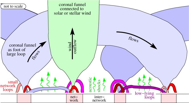
Figure 1: Sketch of the structure of the low corona of the Sun. This cartoon stretches some 60 Mm in the horizontal and 40 Mm in the vertical direction. It indicates the small loops within the network magnetic patches, low-lying loops crossing network cells as well as larger loops rooted in stronger magnetic patches and open coronal funnels. Following Peter (2001).

2 Measurements of coronal magnetic fields

Before discussing modeling of the solar atmosphere including the magnetic field, the attention should be drawn on how to actually observe the magnetic field in the corona. There are various techniques providing the coronal magnetic field.

Direct coronagraphic measurements of the Stokes vector e.g. in the infrared lines of Fe XIII at 10747 Å and 10798 Å applying the Zeeman effect show magnetic fields in bright loops being of the order of 20 Gauss (Lin et al., 2000). Such measurements can be applied only for regions seen above the limb, of course, and are most valuable for the large-scale structure of the corona. Smaller areas, especially low in the corona, are not accessible through this technique, because they are occulted by the design of the coronagraph.

Radio observations allow to investigate the coronal magnetic field also on the disk, e.g. through the Zeeman effect (White, 2005). Radio interferometers such as VLA provide a remarkable spatial resolution of 12 arcsec, and experiments for the future FASR facility showed that the magnetic field strength could be retrieved in a reliable way (White, 2005). The problems here are the detailed interpretation that the emission at a given frequency does originate from a complex volume in the corona, and that these observations are of value mainly for active regions.

Another valuable tool are infrared observations in the He I (10830 Å) triplet using Zeeman and Hanle effect giving magnetic fields for emerging flux regions (Lagg et al., 2004). However, He I is not a coronal line and can thus only indicate magnetic fields in just newly emerging flux regions, which still carry cool plasma.

Extrapolation techniques based on photospheric and/or chromospheric measurements are also a very valuable tool to investigate coronal magnetic fields. As a rule of thumb one might trust these extrapolation on scales typically comparable to or larger than a fraction of the chromospheric network, i.e., some 5–10 Mm. On smaller scales still the expansion of the magnetic field into the chromosphere, i.e. the equilibrium of magnetic and gas pressure, can be expected to dominate. However, whenever interesting events occur, such extrapolations, no matter how fancy, can not be trusted completely, as then the assumption of a force free state is most likely violated. While in such events the overall field structure on the larger scales mentioned above might not change dramatically, the force-free violation might be more severe on smaller scales in a transient manner. This will be certainly true on scales on which explosive events do occur (i.e. some Mm; Innes et al., 1997) as well as on scales not yet resolvable, e.g. in the case of nanoflares. Thus such extrapolations are important and helpful to understand the overall structure and long-term evolution, but real measurements of the coronal magnetic field with a spatial resolution of 1 Mm and better are desperately needed in order to pin-point the relevant processes during phases when the heating mechanism is showing itself through a dynamic non-force-free event, as in flares, explosive events or nanoflares. While the above mainly concerns closed field regions, the same is also true for magnetically open region as found in coronal holes. Following the idea of e.g. Axford and McKenzie (1997) magnetic reconnection of open field with bipolar network flux is the energy source for the heating of the open corona and the wind acceleration. It would be of high interest to detect the non-force-free magnetic reconfiguration predicted by this furnace model through the direct measurement of the magnetic field.

The ideal tool to investigate the magnetic field in the corona is to use lines which are formed in the transition region and corona, i.e. to use the same VUV emission which is currently widely used to investigate the corona with imagers such as TRACE or EIT or spectrometers such as SUMER or CDS. Of course, because of the complicated spatial structure of the corona and the high variability, the interpretation of the polarized light in the VUV will not be possible in a simple and straightforward way, and is thus confronting us with the same problems as radio observations. The coronal models, which become more and more elaborate and realistic, will be of pivotal importance for a proper interpretation of VUV and radio spectro-polarimetric data.

The importance of UV and VUV spectro-polarimetry from space has been emphasized by Trujillo Bueno et al. (2005), who suggest to use the Lyman series of hydrogen for an investigation of the Hanle effect. Another approach is to measure the Stokes vector in strong lines such as the C IV doublet at 1548 Å and 1550 Å, which is formed in the transition region. This is suggested by West et al. (2005), who are currently building an instrument for a series of rocket flights, the first probably in spring 2007 for a test of the system (Solar Ultraviolet Magnetograph Investigation, SUMI). Because of the limited count rate during the rocket flight, they expect to get a signal only in Stokes V, which would be in itself a great step forward, if they succeed.

In the future we have to aim at a combination of spectro-polarimetry in the radio and the VUV. In the radio such techniques already exist, but they have to be refined, also with respect to spatial resolution. For VUV spectro-polarimetry we will certainly have to wait some time until space instrumentation will be available, but this is the instrument to aim at when investigating the magnetic structure of the corona.

3 From 1D to 3D: the closed corona

The most conspicuous basic building block of the corona is the coronal loop. Observations show that more or less semi-circular shaped loops are the most prominent structure in the corona, and they are found in active regions, after flares, in quiescent regions in the network, etc. Therefore most 1D models for the solar corona dealt with loop models, one of the most well-known being the RTV models (Rosner et al., 1978).

Even though it is not clear what the “micro-structure” of an observed loop would be, i.e. if it consists of many individual strands or if it is a bundle of parallel field lines (Klimchuk, 2006), many loop models exist solving the mass, momentum and energy balance along a loop-shaped 1D structure, some now with adaptive mesh refinement and even a self-consistent treatment of the ionization and radiation (e.g. Bradshaw and Mason, 2003; Müller et al., 2003). Such loop models allow a very detailed description of the thermal and dynamic properties within the loop (or strand) modeling complex non-linear processes, e.g. catastrophic cooling (Müller et al., 2004), which is also found in observations (Schrijver, 2001). 1D models for open structures will be discussed in Sect. 6.1.

The main disadvantage of these 1D loop models is that they (usually) are not able to treat the heating process in a physical way. Since the early RTV work almost all 1D models assume a parameterized form of the distribution of coronal heating, e.g. exponentially decaying with height, i.e. not really incorporating a physical heating mechanism into the model. However some models made an attempt to include a distribution of heat into the 1D models as found from other studies.

In the mid 1970ies the Skylab observations showed that the chromospheric network is expanding to higher temperatures (Reeves, 1976), which lead to assume a funnel-type structure of the transition region and low corona (Gabriel, 1976). However, it became clear later that these funnels alone are not a good representation of the corona, even though they are an important ingredient (cf. Fig. 1). For example in the magnetically closed corona the emission measure $EM=\int_{V}\,n_{e}^{2}\,{\rm{d}}V$, i.e. a measure of the emissivity of the corona at a given temperature, could not be reproduced by the funnel models. Because of the ineffective heat conduction at low temperatures the 1D models give an extremely thin transition region, i.e. a very steep temperature gradient, and thus in the model there is not enough material at low temperatures to account for the observed increase of the emission measure towards lower temperatures below some $10^{5}$ K. Dowdy et al. (1986) proposed that loops at various temperatures could account for that increase and through this introduced a complicated magnetic structure of the low corona, sometimes also called “magnetic junkyard” (cf. Fig. 1). Later it was proposed that signatures in the spectra of VUV emission lines support this scenario (Peter, 2000). Furthermore there is ample observational evidence from VUV line emission maps acquired with SUMER that low-lying loops with lengths below 10–20 Mm do exist (e.g. Feldman et al., 2003). However, all these scenarios are not really based on a physical model, but are merely trying to find a plausible way to draw a sketch of the magnetic structure of the low corona.

In open field regions such as coronal holes it seems problematic that the above scenario for the (predominantly) closed field regions holds. There other processes might be more important. Recently Esser et al. (2005) have shown that the (fast) solar wind outflow of the plasma along funnel type structures might well result in significant violation of the ionization equilibrium by lifting a sizable fraction of neutral material higher up into hotter regions of the funnel. This can then produce an increased emission in Ly-$\alpha$ which agrees well with observation. However, it still has to be explored to which extent this process will predict the observed emission from the transition region, i.e. of lines formed at a couple of 100 000 K.

While large-scale structures such as a (polar) coronal hole or an active region complex seem to be rather stable for days and weeks, on smaller scales of below 10 Mm the corona is highly dynamic. When analyzing the spatial magnetic structure on these smaller scales this variability is adding to the complexity of the problem. For example, when modeling an explosive event, it is usually assumed that the “background” magnetic structure remains the same, while only a small perturbation is shuffling around the magnetic field leading to a reconnection event (e.g. Innes and Tóth, 1999). When investigating observations with imagers or spectrographs, one sees a very strong variability in time indicating that the “natural” state of the the transition region and corona on scales below 10 Mm is a dynamic one (Innes, 2004).

4 Why 3D models?

One could argue that a composite model consisting of a large number of loops and open structures would be sufficient to describe the solar corona. Furthermore one could argue to neglect the magnetically open structures in these models as they provide only a minor contribution to the emission in X-rays or the far VUV, i.e. in the wavelength bands accessible to Yohkoh, or the EIT or TRACE coronal channels. As the corona and transition region are built up by (loop-like) magnetic structures which are rooted in the solar photosphere, one could use an extrapolation of the magnetic field to identify the loops and then investigate the resulting structure.

For certain problems this is certainly a good approach. For example Schrijver et al. (2004) did a global extrapolation of the observed photospheric magnetic field to define the loops and used a simple scaling law for the flux of mechanical energy $F_{H}$ into the loop, $F_{H}\propto\,B^{\beta}\,L^{\lambda}\,f$. Here $B$ is the magnetic field at the base of the structure, $L$ its half length, $f=\exp[-(B/500\,G)^{2}]$ a factor accounting for reduced heating in sunspots, and $\beta$ and $\lambda$ are free parameters. Each loop was then described in a static 1D model. The authors then calculated how this constructed multi-loop corona would appear in an X-ray observation (Yohkoh SXT) and compared it to the real observation. By varying $\beta$ and $\lambda$ they found that a heating scaling with $\beta\approx{1.0}{\pm}0.5$ and $\lambda\approx{-0.7}{\pm}0.3$ would give the best fit. Even the best fit is not really representing the real corona, which is not surprising as it is based on a very simple model. Nevertheless it can be used to estimate how the energy input into the corona is roughly scaling with the magnetic structures. Most important, this kind of model opens the possibility for more realistic global models of stellar corona, which are not accessible to direct observations.

For other purposes one-dimensional models, or such multi-loop models would not be sufficient. For example Schrijver and Title (2003) showed that depending on the distribution of internetwork magnetic flux only some 50% of the coronal magnetic field above the quiet Sun does come from network magnetic patches. This implies that the simple idea of a coronal loop being rooted in a single (or even a few) patches of strong magnetic flux in the photosphere is not applicable. Furthermore Jendersie and Peter (2006) could show that based on current instrumentation we are not even able to determine where the coronal field is really rooted, on a scale of a fraction of a super-granule (say 5 Mm). For only small differences in the distribution of weak internetwork flux elements one gets radically different connections from the photosphere into the corona. Therefore when describing the corona in more detail on a scale corresponding to a fraction of a single active region or the chromospheric network, one has to account for the complex magnetic connectivity, because a simple picture of a coronal structure rooted in a single (or few) strong magnetic patch(es) does not really apply. On top of that the problem is even more complicated, because the distribution of magnetic flux in the photosphere changes constantly on time scales from minutes (granules, ${\approx}$1 Mm) to days (super-granules, ${\approx}$20 Mm), which is shorter than the lifetime of many loops. Loop arcades, e.g. as seen by TRACE, overall last longer (many days) than the nano-flaring processes associated with them, so they appear to be rigid, or solid. However, the magnetic connectivity within the loop structures might constantly change while the loop is sitting seemingly still, i.e. the many strands of the loop could constantly change their identity. Currently it is not clear if, and if yes to what extent, this affects the appearance of the loop as a whole. Therefore we might ask ourselves the question what sense the concept of a coronal loop as a rigid magnetic loop really makes.

In consequence, to describe the structure of the transition region and corona, one has to account for the changing “boundary conditions” in the photosphere and include a proper treatment of the 3D structure of the magnetic field.

5 3D MHD coronal box models

One of the most important ingredients for a coronal model is a proper energy equation. Because of the strong flows observed in the active regions as well as quiet corona, the enthalpy flux can play a major role. And only if the energy balance, including furthermore the energy input, heat conduction and radiation are treated well enough, the density of the corona will be correct (as good as possible…). This is because basically the energy input sets the pressure of the coronal structure: for larger energy input more energy will have to be radiated in the transition region. When the heating rate increases this consequently leads to (chromospheric) evaporation, while the coronal temperature changes only little as the heat conduction acts as a thermostat through the strong dependency on temperature (${\propto}T^{5/2}$). Thus only a proper energy equation will assure proper densities and consequently proper velocities within the computational domain.

A severe problem is that the energy dissipation processes are occuring on scales much smaller than currently observable or resolvable with the MHD-type models to describe e.g. an active region complex or a coronal loop. Thus in terms of kinetic physics it is questionable is a “proper energy equation” in fluid terms can even be defined (e.g. Marsch, 2006). However, one might (or have to) hope that when describing the corona with a resolution of the current MHD models (some km in 1D, some 100 km in 3D), the energy deposition as a function of space and time is comparable to the result a micro-physical model smoothed to the MHD scales would give. Also the resistivity in the MHD models is basically set by the (spatial) resolution they can achieve. Due to the limitations for the magnetic Reynolds number this is a common property for all MHD-type models. However MHD studies with different spatial resolutions and resistivities showed that the energy deposition does not change significantly over a range of scales (for resolution and resistivity) accessible to MHD experiments (Galsgaard and Nordlund, 1996; Hendrix et al., 1996). Future work will have to show to what extent the MHD approach is a good representation for the real Sun, but currently it is the most appropriate (and only) tool to describe structures such as active region systems or loop complexes.

The basic test for every coronal model has to be whether it is matching with observations. The most straight-forward way for such a test is to compare observable quantities such a line intensities or shifts synthesized from the model to real observations, as this eliminates the many problems of inversions of VUV spectral data (e.g. Judge and McIntosh, 1999). In the following a 3D MHD coronal box forward model will be discussed which compares very well with observations concerning e.g. the emission measure, line shifts or temporal variability.

5.1 3D forward box model

A 3D MHD model presented by Gudiksen and Nordlund (2005a, b) includes the atmosphere from the photosphere to the lower corona in a 60${\times}$60 Mm horizontal times 37 Mm vertical box. It solves the mass, momentum and energy balance, the latter including classical heat conduction (Spitzer, 1956) and optically thin radiative losses as piecewise power laws. The temperature of the chromosphere is kept near a prescribed profile by Newtonian cooling. Initially the magnetic field is given by a potential field extrapolation with the lower boundary as observed by MDI/SOHO for an active region. Further on in the simulation the field evolves self-consistently and becomes non-potential, of course. The system is driven by horizontal motions at the lower boundary. The flow field is constructed using a Voronoi-tessellation technique (Okabe et al., 1992) and reproduces the typical pattern of the granular motions of the Sun (Schrijver et al., 1997). By this also the power spectra of the velocity and the vorticity are reproduced. The spacing of the (non-uniform) grid goes down to 150 km and is as good it can be given the size of the structure modeled here (60 Mm). Of course all the shortcomings of MHD models as discussed above apply here. For the upper boundary condition it is assumed that the magnetic field above the computational domain is potential, which, of course, prevents the development of larger open magnetic structures (and was not the aim of that study). This has to be kept in mind when discussing the Doppler shifts of coronal lines (Sect. 5.2) and the apparent lack of hot blueshifted material, i.e. a wind.

This procedure leads to a heating of the corona just in the way Parker (1972) suggested. The field line braiding gives high coronal temperatures of a million K, and a system of hot loops is forming, connecting the magnetic concentrations of the active region. Furthermore the system reaches some sort of quasi-stationary state, with large fluctuations in time and space, or in other words, the system is quite dynamic. The detailed discussion of the MHD results can be found in Gudiksen and Nordlund (2005a, b).

Based on the above MHD model results for the density and temperature Peter et al. (2004, 2006) calculated the emissivity at each grid point under the assumption of ionization equilibrium using the atomic data base CHIANTI. Assigning a spectral line profile at each grid point with a line width corresponding to the thermal width, one can integrate the spectra from the 3D box along a line of sight, e.g. the vertical. This results in 2D maps of spectral profiles, which can be analyzed in the same way as observations, e.g. through maps of line intensities or shifts. For a detailed discussion of the synthesis of the emission lines from the transition region and corona and the assumptions and limitations see Peter et al. (2004, 2006).

Figure 2 shows in the middle panel the vertical magnetic field at the bottom of the computational box, i.e. in the photosphere. To the left and right are maps in line intensity and line shift as derived from the spectra computed from the MHD model. They represent a view from the top onto the box, corresponding to an observation at disk center. As found with observations the spatial structures in the transition region line C IV (1548 Å) at 10⁵ K are much smaller and finer than in the corona seen in Mg X (625 Å) formed at 10⁶ K.

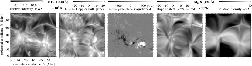
Figure 2: Maps in line intensity and Doppler shift in the transition region (left two panels) and the corona (right two panels) as derived from a snapshot of a 3D MHD coronal model. In these maps the computational box is viewed from above, i.e. this represents the situation when observing near disk center. The middle panel shows the vertical magnetic field at the bottom of the computational domain, i.e. in the photosphere. Following Peter et al. (2006).

5.2 Diagnostics of the 3D model: VUV spectra

In the following a short overview will be given how VUV spectra synthesized from a 3D coronal box model can be used to test the model. It should be stressed that the model results presented in the following show the best overall match to the observations published so far for the differential emission measure, Doppler shifts or rms fluctuations.

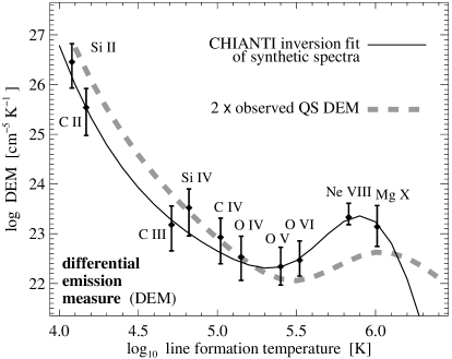
Figure 3: Differential emission measure (DEM) from a 3D MHD box model compared to observations. The solid line shows the fit from the DEM inversion based on the lines displayed as bars, which have been synthesized from the MHD model (integrated over the whole box). The thick dashed line is based on a DEM inversion using observed quiet Sun disk center line radiances observed with SUMER (Wilhelm et al., 1998a) scaled by a factor of two. Following Peter et al. (2004).

Diffential emission measure

For each time step Peter et al. (2004) used the radiances of a number of VUV emission lines synthesized from a MHD model to perform a differential emission measure (DEM) analysis, i.e. they used the maps of the spectral profiles (“synthetic observations”) as described in the previous section and integrated the line profiles over the whole map. Thus the line radiances represent the total emission of the given VUV lines integrated over the whole computational domain. As with real observations one can then use an inversion procedure to derive the differential emission measure (DEM), e.g. with the help of the procedures provided with the CHIANTI atomic data package (Dere et al., 1997; Young et al., 2003). Fig. 3 shows the resulting DEM curve as a solid line for a single time step derived from the intensities of a given set of lines, which characterizes the (average) small active region simulated in the MHD model. For comparison the thick dashed line shows the inversion of actually observed intensities of the same lines. The match of the model with the observations is remarkable, especially, the 3D MHD model used in the Peter et al. (2004) study (Gudiksen and Nordlund, 2002) is reproducing the observed trend of the emission measure below ${\sim}10^{5}$ K, while previous (1D and 2D) models failed to predict this increase of DEM towards lower temperatures (cf. Sect. 3).

In the above model the increase towards the low transition region is caused by numerous low-lying (intermittent) cool structures. This confirms the scenario outlined by Dowdy et al. (1986), in which a hierarchy of large and small, hot and cool loops exist in the transition region and corona as already discussed in Sect. 3. Despite the variability of the low corona, the emission measure (averaged over the computational domain, viz. the active region) changes only little with time.

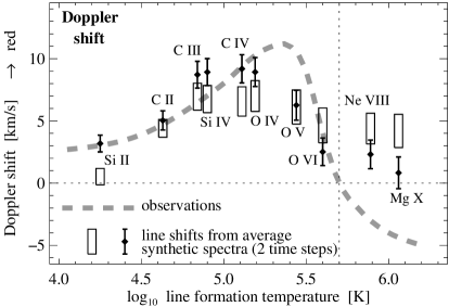
Figure 4: Average Doppler shifts of the synthesized spectra when viewing the computational box from straight above for two different time steps (bars and rectangles). The height of the bars indicate the standard deviation of the Doppler shifts for the respective time step. The thick dashed line shows the trend found in observations (Peter and Judge, 1999). Following Peter et al. (2004).

Average Doppler shifts

Since the discovery of the systematic transition region line redshifts by Doschek et al. (1976), the explanation of these persistent Doppler shifts has been a challenge for modelers. The discovery that the lines formed in the (low) corona show a net blueshift by Peter (1999) and Peter and Judge (1999) using SUMER/SOHO data added a new quality to this challenge. The trend of the net Doppler shift at quiet Sun disk center is shown in Fig. 4 as a thick dashed line (data compiled from Brekke et al., 1997; Chae et al., 1998; Peter and Judge, 1999; Teriaca et al., 1999).

In order to derive the average Doppler shift corresponding to disk center observations one can investigate the Doppler maps of the synthetic spectra with a vertical line-of-sight, i.e. when looking at the computational box from straight above (cf. Fig. 2). The average line shifts as computed by Peter et al. (2004) for two different time steps 7 min apart are plotted in Fig. 4 as bars and rectangles (the heights of the bars and rectangles indicating the scatter of the Doppler shifts).

The line shifts are caused by the dynamic response of the atmosphere to the energy input due to the braiding of magnetic field lines. The flows are partly induced through energy deposition in and subsequent expansion of the corona, partly from evaporation of chromospheric material due to heating at low heights and the heat flux from the corona into the chromosphere.

Throughout the transition region (${<}5{\cdot}10^{5}$ K) the match of the observed Doppler shifts with those of the spectra synthesized from the model is quite good. It should be stressed here that no fine-tuning was applied, but these Doppler shifts follow naturally from the driving of the corona through the footpoint motions of the magnetic field lines. In the low corona (${>}5{\cdot}10^{5}$ K) the synthesized spectra do not show the blueshifts as they are observed (Peter, 1999), but this problem might be overcome (at least partly) by a more appropriate handling of the upper boundary condition.

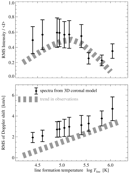
Figure 5: RMS fluctuations in line intensity and shift from the spectra derived from the MHD coronal model for a number of VUV lines as a function of line formation temperature. The thick dashed line shows the trend found in observations by Brković et al. (2003). Following Peter et al. (2005).

Temporal variability

Based on the synthesized maps of line intensities and shifts generated from a line of sight integration along the vertical direction, the rms fluctuations at each spatial pixel within the respective map have been evaluated by Peter et al. (2005). Figure 5 shows their results for a number of VUV lines as a function of line formation temperature. The diamonds show the (spatially) averaged values for the rms fluctuation for each line and the bars represent the scatter of the rms values (standard deviation).

This is exactly the same procedure as used by Brković et al. (2003) to reduce their observational data from CDS and SUMER on SOHO. The trends they found with their observations is over-plotted as thick dashed lines in Fig. 5. It has to be emphasized that the spatial resolution of the maps in line intensity and shift derived from the MHD model has been reduced to match the spatial resolution of the SOHO instruments, as this has an effect on the absolute values of the rms fluctuations (the trend with temperature, however, does not depend on the spatial resolution).

Together with the good match between the average Doppler shifts and emission measure from observations and the spectra computed from the 3D MHD coronal box model presented above, this is yet another strong indication that the underlying 3D coronal model is a good description for the coronal heating mechanism.

5.3 The magnetic structure

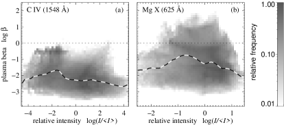
Figure 6: 2D histograms of plasma–$\beta$ as a function of line intensity (a: C IV, b: Mg X). The dashed lines show the median value of plasma–$\beta$ in a given interval of intensity. Please note that the 2D histograms are plotted on a log-scale. Following Peter et al. (2006).

To investigate the interaction of the magnetic field and the plasma one can discuss plasma–$\beta$, i.e. the ratio of the gas pressure to the magnetic pressure, $\beta=2\mu\,p/B^{2}$. Fig. 6 shows the relation of $\beta$ to the synthesized transition region (a; C IV) and coronal (b; Mg X) emission within the computational box as done by Peter et al. (2006). The plots show the 2D histograms of the plasma beta as a function of (normalized) intensity of the respective line, i.e. the color coding represents the fraction of the volume where one finds the respective combination of plasma-$\beta$ and normalized intensity. The median relations between plasma-$\beta$ and the normalized intensities are over-plotted as dashed lines. The transition region and corona are mostly in a low-$\beta$ state, however with noticeable exceptions in the coronal part!

It is clear that in the whole transition region the assumption of a low-$\beta$ plasma is very good (Fig. 6a). This is different, however, in the corona when relating $\beta$ to the Mg X emission (Fig. 6b). A large fraction of the not-low-beta plasma in the corona is at low densities, i.e. at $\log\,I/{\langle}I{\rangle}<0$, where the magnetic field is very weak, too. As these are regions of low emission, one might be inclined to disregard this. However, even in the volume with a relative intensity larger than the median intensity (i.e. $\log\,I/{\langle}I{\rangle}>0$ in Fig. 6b) contributing ${\sim}$90% to the total coronal Mg X emission, some ${\sim}$5% of this bright material has values of $\beta>1$ (Peter et al., 2006). These are regions of rather high densities but low magnetic field, and they can be found e.g. in regions along magnetic neutral lines across which the direction of the magnetic field changes and thus strong currents heat the plasma and finally cause the density to increase.

In conclusion, in significant patches of the corona, even above active regions, $\beta$ is in fact not much less than unity.

This again emphasizes that for “good” coronal model it is not enough to only extrapolate the magnetic field and then solve a lot of 1D loop-like problems along each field line. Instead, one has to account for the interaction of the plasma and the magnetic field in a more complex 3D model.

6 3D MHD models for open structures

So far the discussion concentrated on magnetically closed structures, such as active regions or the chromospheric network. In magnetically open regions the plasma is not trapped by the magnetic field, but can escape along magnetic field lines. This is the basic reason why coronal holes, i.e. the source region of the fast solar wind, appear dark. Because a large part of the energy goes into acceleration of the wind, there is less energy to heat the plasma. Consequently the temperature is a bit lower than in the quiet Sun, typically below $10^{6}$ K (Wilhelm et al., 1998b). The effect of the reduced heating rate is much stronger on the pressure, which results in a lower density in the corona above the holes — we see less emission from the coronal holes.

6.1 1D scenarios and models for the fast wind

As for the quiet and active Sun structures, which are dominated by loops, the first models for the open corona, which is the same as for the fast wind, were 1D models stretching from the base of the corona into interplanetary space, with an area expansion factor accounting for the (super) radial expansion of the magnetic field.

As with the loops these models used a parameterized form of the energy input, which was typically concentrated close to the Sun. As mentioned earlier, in order to properly understand the mass loss, especially to describe the mass loss rate self-consistently set by the energy input, one has to include a transition region to account for the heat flux back to the Sun (Hammer, 1982a, b; Withbroe, 1988). Only then one can describe properly the interplay between coronal heating, densities, temperatures and solar wind acceleration, as done first by Hansteen and Leer (1995). However, as for the 1D loop models (cf. Sect. 3), these models did not include a physical heating mechanism.

In contrast, Axford and McKenzie (1997) put forward an idea that small-scale reconnection in the magnetic concentrations of the chromospheric network (i.e. between open and closed field lines) leads to high-frequency Alfvén waves which propagate upwards into the corona, a concept also called magnetic furnace. These waves can then resonantly interact with the protons and heavy ions in the open corona and drive the wind as has been described by Marsch and Tu (1997b) and Tu and Marsch (1997). Furthermore one can also account for the expansion of the magnetic field directly above the magnetic concentrations in the chromosphere forming large funnels (Marsch and Tu, 1997a; Hackenberg et al., 2000).

These 1D models including a physical mechanism for the heating and acceleration of the plasma describe a situation where the material is continuously and constantly accelerated from the chromosphere out into the solar wind (e.g. Holzer, 2005). By this they implicitly assume that the magnetic configuration from the upper chromosphere into the solar wind is rather stable! This would strongly contradict the scenario outlined for the closed field regions in the previous section, where the magnetic field in the photosphere is constantly shuffled, resulting in a continuous change also higher up.

6.2 Observing the source of the fast wind

It has been known for a while that the fast wind is originating from coronal holes, and observations of blueshifts in coronal lines within coronal holes confirmed this (Rottman et al., 1982; Orrall et al., 1983). Even the transition region lines of C IV showed a higher fraction of blueshifted regions in coronal holes than in the quiet Sun (Dere et al., 1989; Peter, 1999).

The strongest blueshifts are found in the darkest coronal regions (Wilhelm et al., 2000) and they seem to be concentrated at intersections of network lanes (Hassler et al., 1999). A comparison of the Doppler shift patterns to the photospheric magnetic field showed that these strong blueshifts, interpreted as the base of the outflow, coincide with strong magnetic concentrations in the network (Xia et al., 2004). These data seemed to support the wind scenario described above, namely that funnel-type structures emerging from strong network magnetic patches define the flow channels of the wind reaching out into the interplanetary medium.

One can investigate the magnetic connectivity from the photosphere to the corona in coronal holes and compare this to the Doppler shift signals of transition region and (low) coronal lines. This shows that the blueshifts in coronal lines coincide with the magnetic funnels, but that at those locations no systematic blueshifts can be found in transition region lines within the instrumental uncertainties (Tu et al., 2005). Based on this observation Tu et al. (2005) argued that the plasma of the solar wind outflow has to be injected somewhere between the formation heights of the transition region and coronal lines they inspected (C IV and Ne VIII), i.e. somewhere around 10 Mm. If this is correct, it changes dramatically our view of the formation of the wind at its very base, because it would challenge the old paradigm that there is a continuous outflow of the wind from the chromosphere into the heliosphere. However, because of the higher densities in the transition region the expected outflow speed of the wind should be rather low ($\approx$1 km/s) at the level where one can expect C IV to form. This is just at the resolution limit of current instrumentation, e.g. SUMER/SOHO can determine Doppler shifts down to some 1–2 km/s (Peter and Judge, 1999). Therefore it remains unclear, whether there is a continuous outflow from the chromosphere, with a small not yet detectable velocity at C IV heights, or if the velocity in C IV is really zero and the wind is injected between the levels of C IV and Ne VIII as suggested by Tu et al. (2005).

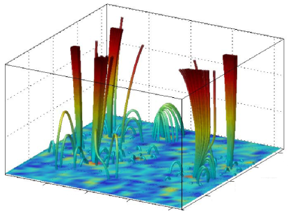
Figure 7: Initial setup of the magnetic field in the 3D box model for an open field region by Büchner and Nikutowski (2005). The bottom boundary of the magnetic field is taken from observations and is driven by whirl flows, which brings together the open and closed regions leading to reconnection. From Büchner and Nikutowski (2005).

6.3 Accounting for the magnetic structure: 3D models for the onset of the fast wind

To investigate the scenario proposed by Tu et al. (2005) a numerical experiment was conducted by Büchner and Nikutowski (2005). They start with a magnetic configuration given at the lower boundary from observations and then drive the system by whirl flows imposed on the lower boundary. Through this they bring together open and closed magnetic field structures which results in reconnection. Their model contains a plasma–neutral gas coupling, i.e. it includes effects beyond MHD. For the reconnection they used a switch-on-resistivity, i.e. the resistivity is non-zero only where the current-carrier-velocity (${\propto}j/n$) is above a certain threshold. By this their treatment of the reconnection is more detailed than the 3D box models for the closed corona discussed in Sect. 5.1, however, they used a simplified energy equation, not accounting for heat conduction or energy losses through optically thin radiation (cf. Büchner et al., 2005). The magnetic configuration (at the initial state) is shown in Fig. 7.

As a consequence of driving the magnetic field through the whirls at the bottom, the reconnection between the open and closed regions injects energy and plasma into the open funnels and through this drives a wind out of the funnels. Roughly, the plasma below $10^{5}$ K falls down, plasma above $10^{5}$ K leaves the computational box through the top. The downdrafts are mostly concentrated above the magnetic concentrations at the bottom boundary. Thus this simulation supports the general picture suggested by Tu et al. (2005). However, further modeling with a proper inclusion of an energy equation and also an investigation of the VUV emission to be expected from this model is needed before a final conclusion can be drawn.

At the moment we have to conclude that even in the very quiet coronal holes, the assumption of a stationary magnetic field configuration simply channeling the solar wind outflow is not justified. To really understand the origin of the solar wind we have to account for the complex interaction between different magnetic field structures and also between the magnetic field and the plasma.

7 Conclusions

A realistic model of the (upper) solar atmosphere has to account for the complexity of its magnetic structure. Together with the constant rearrangement of the magnetic field at photospheric levels this leads to an ongoing energy release in the low parts of the transition region and corona and through this drives the highly dynamic upper atmosphere.

The current box models for magnetically closed regions as discussed in Sect. 5 show a qualitatively good match to observed quantities, such as emission measures, Doppler shifts of rms-variability. This presents ample evidence that the heating through field line braiding is a prime candidate to heat the corona. Of course, other means of energy input into the corona might also reproduce the average quantities of e.g. emission measure, Doppler shift or line widths as presented in this paper. It remains to be seen if other models based on different heating processes will give the same or different results, once they are pushed to produce observables as now done for the field line braiding model. In the future more efforts have to be undertaken not only to increase the spatial resolution of the simulations, but also to actually include a physical mechanism for the dissipation of magnetic energy during the reconnection events.

The box models for magnetically open region, i.e. for the onset of the fast wind (Sect. 6), have not yet been analyzed in such detail concerning observable properties, but they support some recent interpretation of observational data suggesting that plasma is injected in funnel-type structures to form the fast solar wind.

Together with the very successful global coronal models, which have only briefly been touched upon in this paper, now complex three-dimensional models become available accounting properly for the plasma and the magnetic field as well as their interaction. We might hope that the coming years will bring further advances of these models and their diagnostic capabilities. Thus we will improve our understanding of the structure, dynamics and heating of the upper atmospheres of the Sun and solar-like stars.

References

- Axford and McKenzie (1997) Axford, W. I., McKenzie, J. F., 1997. The solar wind. In: Jokipii, J. R., Sonett, C. P., Giampapa, M. S. (Eds.), Cosmic winds and the heliosphere. Univ. of Ariziona Press, Tucson, pp. 31–66.
- Bradshaw and Mason (2003) Bradshaw, S. J., Mason, H. E., 2003. The radiative response of solar loop plasma subject to transient heating. A&A 407, 1127–1138.
- Brekke et al. (1997) Brekke, P., Hassler, D. M., Wilhelm, K., 1997. Doppler shifts in the quiet sun transition region and corona observed with sumer on soho. Solar Phys. 175, 349–374.
- Brković et al. (2003) Brković, A., Peter, H., Solanki, S. K., 2003. Variability of EUV-spectra from the quiet upper solar atmosphere: intensity and Doppler shift. A&A 403, 725–730.
- Büchner (2006) Büchner, J., 2006. Theory and simulation of reconnection. Space Sci. Rev. 124, 345–360.
- Büchner and Nikutowski (2005) Büchner, J., Nikutowski, B., 2005. Acceleration of the fast solar wind by reconnection. In: Connecting Sun and heliosphere. Proceedings of Solar Wind 11 / SOHO 16, ESA SP-592, pp. 141–146.
- Büchner et al. (2005) Büchner, J., Nikutowski, B., Otto, A., 2005. Coronal heating by transition region reconnection. In: Coronal heating, Proc. of SOHO 15. ESA SP-575.
- Chae et al. (1998) Chae, J., Yun, H. S., Poland, A. I., 1998. Temperature dependence of ultraviolet line average doppler shifts in the quiet sun. ApJS 114, 151–164.
- Dere et al. (1989) Dere, K. P., Bartoe, J.-D. F., Brueckner, G. E., Recely, F., 1989. Transition zone flows observed in a coronal hole on the solar disk. ApJ 345, L95–L97.
- Dere et al. (1997) Dere, K. P., Landi, E., Mason, H. E., Monsignori Fossi, B. C., Young, P. R., 1997. Chianti - an atomic database for emission lines. A&AS 125, 149–173.
- Doschek et al. (1976) Doschek, G. A., Feldman, U., Bohlin, J. D., 1976. Doppler wavelength shifts of transition zone lines measured in Skylab solar spectra. ApJ 205, L177–L180.
- Dowdy et al. (1986) Dowdy, J. F., Rabin, D., Moore, R. L., 1986. On the magnetic structure of the quiet transition region. Solar Phys. 105, 35–45.
- Esser et al. (2005) Esser, R., Lie-Svendsen, Ø., Janse, Å., Killie, M., 2005. Solar wind from coronal funnels and transition region Ly? ApJ 629, L61–L64.
- Feldman et al. (2003) Feldman, U., Dammasch, I. E., Wilhelm, K., et al., 2003. SUMER atlas – Images of the solar upper atmosphere from SUMER on SOHO. ESA Publications Div., ESA SP-1274.
- Gabriel (1976) Gabriel, A. H., 1976. A magnetic model of the solar transition region. Phil. Trans. Roy. Soc. Lond. A 281, 339–352.
- Galsgaard and Nordlund (1996) Galsgaard, K., Nordlund, Å., 1996. Heating and activity of the solar corona. I. Boundary shearing of an initially homogeneous magnetic field. J. Geophys. Res. 101, 13445–13460.
- Gudiksen and Nordlund (2002) Gudiksen, B., Nordlund, Å., 2002. Bulk heating and slender magnetic loops in the solar corona. ApJ 572, L113–116.
- Gudiksen and Nordlund (2005a) Gudiksen, B., Nordlund, Å., 2005a. An ab initio approach to the solar coronal heating problem. ApJ 618, 1020–1030.
- Gudiksen and Nordlund (2005b) Gudiksen, B., Nordlund, Å., 2005b. An ab initio approach to solar coronal loops. ApJ 618, 1031–1038.
- Hackenberg et al. (2000) Hackenberg, P., Marsch, E., Mann, G., 2000. On the origin of the fast solar wind in polar coronal funnels. A&A 360, 1139–1147.
- Hammer (1982a) Hammer, R., 1982a. Energy balance of stellar coronae I. methods and examples. ApJ 259, 767–778.
- Hammer (1982b) Hammer, R., 1982b. Energy balance of stellar coronae II. effect of coronal heating. ApJ 259, 779–791.
- Hansteen and Leer (1995) Hansteen, V. H., Leer, E., 1995. Coronal heating, densities and temperatures and solar wind acceleration. J. Geophys. Res. 100, 21577–21593.
- Hassler et al. (1999) Hassler, D. M., Dammasch, I. E., Lemaire, P., et al., 1999. Solar wind outflow and the chromospheric magnetic network. Science 283, 810–813.
- Hendrix et al. (1996) Hendrix, D. L., van Hoven, G., Mikic, Z., Schnack, D. D., 1996. The viability of ohmic dissipation as a coronal heating source. ApJ 470, 1192–1197.
- Holzer (2005) Holzer, T. E., 2005. Heating and acceleration of the solar plasma. In: Connecting Sun and heliosphere. Proceedings of Solar Wind 11 / SOHO 16, ESA SP-592, pp. 115–130.
- Innes (2004) Innes, D. E., 2004. Transition region dynamics. In: Waves, Oscillations and Small-Scale Transient Events in the Solar Atmosphere, Proc. SOHO 13. ESA SP-547, pp. 215–221.
- Innes et al. (1997) Innes, D. E., Inhester, B., Axford, W. I., Wilhelm, K., 1997. Bi-directional plasma jets produced by magnetic reconnection on the sun. Nature 386, 811–813.
- Innes and Tóth (1999) Innes, D. E., Tóth, 1999. Simulations of small-scale explosive events on the sun. Solar Phys. 185, 127–141.
- Jendersie and Peter (2006) Jendersie, S., Peter, H., 2006. Link between the chromospheric network and magnetic structures of the corona. A&A 460, 901–908.
- Judge and McIntosh (1999) Judge, P. G., McIntosh, S. W., 1999. Non-uniqueness of atmospheric modeling. Solar Phys. 190, 331–350.
- Klimchuk (2006) Klimchuk, J. A., 2006. On solving the coronal heating problem. Solar Phys. 234, 41–77.
- Lagg et al. (2004) Lagg, A., Woch, J., Krupp, N., Solanki, S. K., 2004. Retrieval of the full magnetic vector with the he i multiplet at 1083 nm. maps of an emerging flux region. A&A 414, 1109–1120.
- Lin et al. (2000) Lin, H., Penn, M. J., Tomczyk, S., 2000. A new precise measurement of the coronal magnetic field strength. ApJ 541, L83–L86.
- Linker et al. (2005) Linker, J. A., Lionello, R., Mikic, Z., Riley, P., 2005. Time-dependent response of the large-scale solar corona. In: Chromospheric and Coronal Magnetic Fields. ESA SP-596.
- Lionello et al. (2005) Lionello, R., Riley, P., Linker, J. A., Mikić, Z., 2005. The effects of differential rotation on the magnetic structure of the solar corona: Magnetohydrodynamic simulations. ApJ 625, 463–473.
- Marsch (2006) Marsch, E., 2006. Kinetic physics of the solar corona and solar wind. Living Rev. Solar Phys. 3, http://www.livingreviews.org/lrsp–2006–1.
- Marsch and Tu (1997a) Marsch, E., Tu, C., 1997a. Solar wind and chromospheric network. Solar Phys. 176, 87–106.
- Marsch and Tu (1997b) Marsch, E., Tu, C.-Y., 1997b. The effects of high-frequency alfvén waves on coronal heating and solar wind acceleration. A&A 319, L17–L20.
- Mihalas and Weibel Mihalas (1984) Mihalas, D., Weibel Mihalas, B., 1984. Foundations of radiation hydrodynamics. Oxford University Press.
- Müller et al. (2003) Müller, D., Hansteen, V. H., Peter, H., 2003. Dynamics of solar coronal loops. I. Condensation in cool loops and its effect on transition region lines. A&A 411, 605–613.
- Müller et al. (2004) Müller, D., Peter, H., Hansteen, V. H., 2004. Dynamics of solar coronal loops. II. Catastrophic cooling and high-speed downflows. A&A 424, 289–300.
- Okabe et al. (1992) Okabe, A., Boots, B., Sugihara, K., 1992. Spatial tessellations. Concepts and applications of voronoi diagrams. Wiley Series in Probability and Mathematical Statistics, Chichester, New York.
- Orrall et al. (1983) Orrall, F. Q., Rottman, G. J., Klimchuk, J. A., 1983. Outflow from the sun’s polar corona. ApJ 266, L65–L68.
- Parker (1972) Parker, E. N., 1972. Topological dissipation and the small-scale fields in turbulent gases. ApJ 174, 499–510.
- Peter (1999) Peter, H., 1999. Analysis of transition-region emission line profiles from full-disk scans of the sun using the sumer instrument on soho. ApJ 516, 490–504.
- Peter (2000) Peter, H., 2000. Multi-component structure of solar and stellar transition regions. A&A 360, 761–776.
- Peter (2001) Peter, H., 2001. On the nature of the transition region from the chromosphere to the corona of the Sun. A&A 374, 1108–1120.
- Peter et al. (2004) Peter, H., Gudiksen, B., Nordlund, Å., 2004. Coronal heating through braiding of magnetic field lines. ApJ 617, L85–L88.
- Peter et al. (2005) Peter, H., Gudiksen, B., Nordlund, Å., 2005. Coronal heating through braiding of magnetic field lines: synthesized coronal euv emission and magnetic structure. In: Chromospheric and Coronal Magnetic Fields. ESA SP-596.
- Peter et al. (2006) Peter, H., Gudiksen, B., Nordlund, Å., 2006. Forward modeling of the corona of the sun and solar-like stars: from a three-dimensional magnetohydrodynamic model to synthetic extreme-ultraviolet spectra. ApJ 638, 1086–1100.
- Peter and Judge (1999) Peter, H., Judge, P. G., 1999. On the Doppler shifts of solar UV emission lines. ApJ 522, 1148–1166.
- Reeves (1976) Reeves, E. M., 1976. The EUV chromospheric network in the quiet sun. Solar Phys. 46, 53–72.
- Rosner et al. (1978) Rosner, R., Tucker, W. H., Vaiana, G. S., 1978. Dynamics of the quiescent solar corona. ApJ 220, 643–665.
- Rottman et al. (1982) Rottman, G. J., Orrall, F. Q., Klimchuk, J. A., 1982. Measurements of outflow from the base of solar coronal holes. ApJ 260, 326–337.
- Schrijver et al. (2004) Schrijver, C., Sandman, A. W., Aschwanden, M. J., DeRosa, M. L., 2004. The coronal heating mechanism as identified by full-sun visualizations. ApJ 615, 512–525.
- Schrijver (2001) Schrijver, C. J., 2001. Simulations of the photospheric magnetic activity and outer atmospheric radiative losses of cool stars based on characteristics of the solar magnetic field. ApJ 547, 475–490.
- Schrijver et al. (2006) Schrijver, C. J., Derosa, M. L., Metcalf, T. R., et al., 2006. Nonlinear force-free modeling of coronal magnetic fields. Part I: A quantitative comparison of methods. Solar Phys. 235, 161–190.
- Schrijver et al. (1997) Schrijver, C. J., Hagenaar, H. J., Title, A. M., 1997. On the patterns of the solar granulation and supergranulation. ApJ 475, 328–337.
- Schrijver and Title (2003) Schrijver, C. J., Title, A. M., 2003. The magnetic connection between the solar photosphere and the corona. ApJ 597, L165–L168.
- Spitzer (1956) Spitzer, L., 1956. Physics of fully ionized gases. Interscience, New York.
- Teriaca et al. (1999) Teriaca, L., Banerjee, D., Doyle, J. G., 1999. Sumer observations of doppler shift in the quiet sun and in an active region. A&A 349, 636–648.
- Trujillo Bueno et al. (2005) Trujillo Bueno, J., Landi Degl’Innocenti, E., Casini, R., Martínez Pillet, V., 2005. The scientific case for quantum spectropolarimetry from space. In: Chromospheric and Coronal Magnetic Fields. ESA SP–596.
- Tu and Marsch (1997) Tu, C.-Y., Marsch, E., 1997. Two-fluid model for heating of the solar corona and acceleration of the solar wind by high-frequency alfvén waves. Solar Phys. 171, 363–391.
- Tu et al. (2005) Tu, C.-Y., Zhou, C., Marsch, E., et al., 2005. Solar wind origin in coronal funnels. Science 308, 519–523.
- West et al. (2005) West, E. A., Porter, J. G., Davis, J. M., et al., 2005. The solar ultraviolet magnetograph investigation: polarization properties. SPIE 5901, 226–235.
- White (2005) White, S. M., 2005. Radio measurements of coronal magnetic fields. In: Chromospheric and Coronal Magnetic Fields. ESA SP–596.
- Wilhelm et al. (2000) Wilhelm, K., Dammasch, I. E., Marsch, E., Hassler, D. M., 2000. On the source regions of the fast solar wind in polar coronal holes. A&A 353, 749–756.
- Wilhelm et al. (1998a) Wilhelm, K., Lemaire, P., Dammasch, I. E., et al., 1998a. Solar irradiance and radiances of uv and euv lines during the minimum of the sunspot activity in 1996. A&A 334, 685–702.
- Wilhelm et al. (1998b) Wilhelm, K., Marsch, E., Dwivedi, B. N., et al., 1998b. The solar corona above polar coronal holes as seen by sumer on soho. ApJ 500, 1023–1038.
- Withbroe (1988) Withbroe, G. L., 1988. The temperature structure, mass and energy flow in the corona and inner solar wind. ApJ 325, 442–467.
- Xia et al. (2004) Xia, L. D., Marsch, E., Wilhelm, K., 2004. On the network structures in solar equatorial coronal holes. observations of sumer and mdi on soho. A&A 424, 1025–1037.
- Young et al. (2003) Young, P. R., Del Zanna, G., Landi, E., Dere, K. P., Mason, H. E., Landini, M., 2003. Chianti - an atomic database for emission lines. vi. proton rates and other improvements. ApJS 144, 135–152.