Electron Heating in Hot Accretion Flows

Abstract

Local (shearing box) simulations of the nonlinear evolution of the magnetorotational instability in a collisionless plasma show that angular momentum transport by pressure anisotropy ($p_{\perp}\neq p_{\parallel}$, where the directions are defined with respect to the local magnetic field) is comparable to that due to the Maxwell and Reynolds stresses. Pressure anisotropy, which is effectively a large-scale viscosity, arises because of adiabatic invariants related to $p_{\perp}$ and $p_{\parallel}$ in a fluctuating magnetic field. In a collisionless plasma, the magnitude of the pressure anisotropy, and thus the viscosity, is determined by kinetic instabilities at the cyclotron frequency. Our simulations show that $\sim 50$ % of the gravitational potential energy is directly converted into heat at large scales by the viscous stress (the remaining energy is lost to grid-scale numerical dissipation of kinetic and magnetic energy). We show that electrons receive a significant fraction ($\sim~{}[T_{e}/T_{i}]^{1/2}$) of this dissipated energy. Employing this heating by an anisotropic viscous stress in one dimensional models of radiatively inefficient accretion flows, we find that the radiative efficiency of the flow is greater than 0.5% for $\dot{M}\gtrsim 10^{-4}\dot{M}_{Edd}$. Thus a low accretion rate, rather than just a low radiative efficiency, is necessary to explain the low luminosity of many accreting black holes. For Sgr A* in the Galactic Center, our predicted radiative efficiencies imply an accretion rate of $\approx 3\times 10^{-8}M_{\odot}\,{\rm yr^{-1}}$ and an electron temperature of $\approx 3\times 10^{10}$ K at $\approx 10$ Schwarzschild radii; the latter is consistent with the brightness temperature inferred from VLBI observations.

1 Introduction

Local and global simulations have shown that the magnetorotational instability (MRI) is the likely source of turbulence and angular momentum transport in many astrophysical accretion disks (e.g., Balbus & Hawley, 1991, 1998; Hawley, Gammie, & Balbus, 1995; Armitage, 1998). The MRI has been studied in a wide variety of contexts, from the disk of the Milky Way (Piontek & Ostriker, 2005) to planet-forming disks around young stars (e.g., Winters, Balbus, & Hawley 2003). Our recent work has focused on the evolution of the MRI in collisionless plasmas (Quataert, Dorland, & Hammett 2002, Sharma, Hammett, & Quataert 2003, Sharma et al. 2006 [hereafter SHQS]; for related work, see Balbus 2004 and Krolik & Zweibel 2006). These calculations are motivated by the application to radiatively inefficient accretion flow (RIAF) models (Ichimaru, 1977; Rees et. al., 1982; Narayan & Yi, 1995), which are believed to be applicable to accretion onto black holes and neutron stars when the accretion rate is less than a few % of Eddington. Sgr A* in our Galactic Center is the paradigm case for accretion via a RIAF (see Quataert 2003 for a review).

One of the central problems in the theory of hot accretion flows remains understanding the extreme low luminosity of accretion onto black holes in many galactic nuclei (Fabian & Canizares 1988; Fabian & Rees 1995; Loewenstein et al. 2001) and X-ray binaries (e.g., Narayan, McClintock, & Yi 1996). In the context of RIAF models, the observed low luminosities can be explained if most of the available mass is not accreted because of outflows or convection (Blandford & Begelman 1999; Quataert & Gruzinov 2000; Stone, Pringle, & Begelman 1999; Narayan, Igumenshchev, & Abramowicz 2000), or if the gravitational potential energy primarily heats the poorly radiating ions (Rees et. al., 1982; Narayan & Yi, 1995). Global MHD simulations support the former possibility (Stone & Pringle, 2001; Hawley, Balbus, & Stone, 2001).

A number of analytic arguments have been presented for the heating of electrons and ions in the collisionless plasmas appropriate to RIAFs. These estimates focus on heating by MHD turbulence (Quataert, 1998; Gruzinov, 1998; Blackman, 1999; Quataert & Gruzinov, 1999; Medvedev, 2000) or reconnection (Bisnovatyi-Kogan & Lovelace, 1997; Quataert & Gruzinov, 1999). Our shearing box simulations of MRI turbulence in a collisionless plasma suggest an additional mechanism for particle heating in RIAFs. Adiabatic invariance ($\mu=v_{\perp}^{2}/B\propto p_{\perp}/B=$ constant) in a collisionless plasma with a fluctuating magnetic field results in a macroscopic pressure anisotropy, with the pressure perpendicular to the field lines ($p_{\perp}$) exceeding that along the field lines ($p_{\parallel}$). This pressure anisotropy results in a viscous transport of angular momentum that is comparable to the transport by magnetic stresses (SHQS). In a collisional plasma, the magnitude of pressure anisotropy, and thus the viscosity, is determined by Coulomb collisions. In turn, the relative heating of electrons and ions by viscosity is set by the temperature and particle-mass dependence of the Coulomb cross-section (which results in primarily ion heating). In a collisionless plasma, however, the pressure anisotropy—and thus the viscosity—is regulated by the growth of small scale instabilities that violate adiabatic invariance and isotropize the plasma pressure (e.g., the firehose, mirror, ion cyclotron, and electron whistler instabilities). As we shall show, these instabilities also regulate the viscous heating of electrons and ions in a collisionless accretion flow.

In §2 we summarize the equations that describe the evolution of the pressure tensor ($p_{\parallel}$ and $p_{\perp}$); a more detailed presentation is given in SHQS. We then present upper limits on the pressure anisotropy because of gyroradius scale instabilities. We use these limits to provide analytic estimates for the viscous heating of electrons and ions in a collisionless plasma and contrast these results with the more familiar results appropriate to a collisional plasma. In §3 we discuss the results of two-component (electron + proton) shearing-box simulations of the MRI. This is an extension of our single component simulations (SHQS). In §4 we use 1-D models of RIAFs to calculate the radiative efficiency using the viscous heating of electrons calculated in §2 and §3. We also show that electron Coulomb collisions are less effective at reducing the pressure anisotropy in RIAFs than kinetic microinstabilities and thus that the kinetic approach focused on throughout this paper is appropriate. Finally, §5 is a discussion of our key results and their application to RIAFs.

2 Analytic considerations

In the limit that the fluctuations of interest have length scales much larger than the gyroradius and time scales much longer than the cyclotron period, the equations describing the evolution of $p_{\parallel}$ and $p_{\perp}$ are given by (Kulsrud, 1983; Snyder, Hammett, & Dorland, 1997, and references therein)

$$\frac{\partial p_{\parallel,s}}{\partial t} + \nabla\cdot(p_{\parallel,s}{\bf V})+\nabla\cdot{\bf q}_{\parallel,s}+2p_{\parallel,s}{\bf\hat{b}\hat{b}}:\nabla{\bf V}$$ (1)

$$- 2q_{\perp,s}\nabla\cdot{\bf\hat{b}}=-\frac{2}{3}\nu_{eff,s}(p_{\parallel,s}-p_{\perp,s}),$$

$$\frac{\partial p_{\perp,s}}{\partial t} + \nabla\cdot(p_{\perp,s}{\bf V})+\nabla\cdot{\bf q}_{\perp,s}+p_{\perp,s}\nabla\cdot{\bf V}$$ (2)

$$- p_{\perp,s}{\bf\hat{b}\hat{b}}:\nabla{\bf V}+q_{\perp,s}\nabla\cdot{\bf\hat{b}}$$

$$= -\frac{1}{3}\nu_{eff,s}(p_{\perp,s}-p_{\parallel,s}),$$

where the subscript ‘$s$’ denotes the species (electrons and ions [we only consider protons]), ${\bf\hat{b}}$ is the local magnetic field direction, ${\bf V}$ is the fluid velocity, ${\bf q_{\perp}}=q_{\perp}{\bf\hat{b}}\,({\bf q_{\parallel}}=q_{\parallel}{\bf\hat{b}})$ is the flux of perpendicular (parallel) thermal energy along the local magnetic field. The effective pitch-angle scattering rate due to high frequency waves (or Coulomb collisions) is given by $\nu_{eff}$.

Equations (1) and (2) can be obtained by taking the moments of the drift kinetic equation, the Vlasov equation in the limit of large wavelength and long timescales. These moment equations run into the usual “closure” problem. In our numerical calculations, we use a simple closure for the heat flux, in which the heat flux is proportional to the temperature gradient, with the conductivity being a free parameter. This model can roughly reproduce kinetic effects such as collisionless damping of linear modes (see Sharma, Hammett, & Quataert, 2003; Sharma, 2006). For the analytic estimates in this section, these details of the heat fluxes are not important. In addition, our numerical simulations show that the electron heating rate does not depend strongly on the details of the heat flux model.

Equations (1) & (2) can be combined to derive equations for the internal energy ($e_{s}\equiv 3p_{s}/2\equiv p_{\parallel,s}/2+p_{\perp,s}$) and pressure anisotropy ($\Delta p_{s}=p_{\parallel,s}-p_{\perp,s}$), which are given by

$$\frac{\partial e_{s}}{\partial t} + {\bf\nabla\cdot}\left(e_{s}{\bf V+q_{s}}\right)+p_{\perp,s}{\bf\nabla\cdot V}$$ (3)

$$= -\Delta p_{s}{\bf\hat{b}\hat{b}:\nabla V},$$

$$\frac{\partial\Delta p_{s}}{\partial t} + {\bf\nabla\cdot}\left(\Delta p_{s}{\bf V}+{\bf\Delta q_{s}}\right)=-3p_{s}{\bf\hat{b}\hat{b}:\nabla V}$$ (4)

$$+ p_{\perp,s}{\bf\nabla\cdot V}+3q_{\perp,s}{\bf\nabla\cdot\hat{b}}$$

$$- \nu_{eff,s}\Delta p_{s},$$

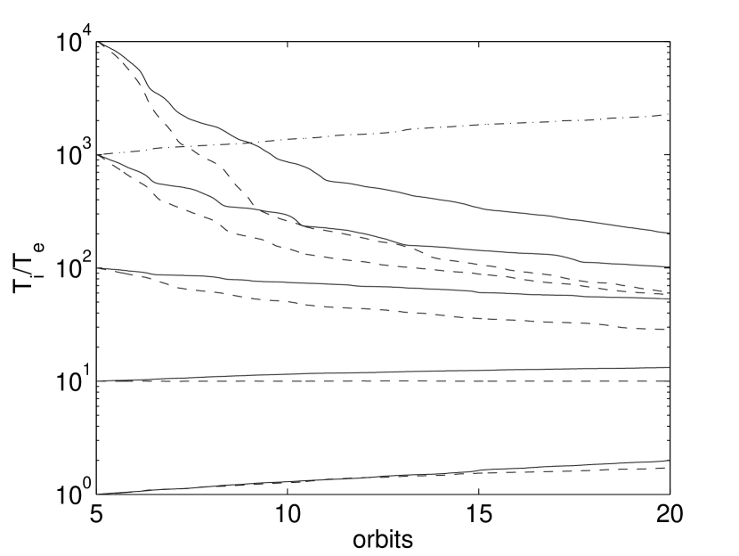
Figure 4: The ratio of the volume averaged ion and electron temperatures as a function of time for models where the ion and electron temperature ratios are set to $10^{4}$, $10^{3}$, $10^{2}$, 10, and 1 at the end of 5 orbits (top to bottom). Solid lines are for $k_{L}=0.5/\delta z$ and dashed lines are for $k_{L}=\infty$ (the CGL limit). The electron heating is somewhat larger in the CGL limit (see also Fig. [5]). Also shown (dot dashed line) is a calculation with $T_{i}/T_{e}=10^{3}$ at 5 orbits for $k_{L}=0.5/\delta z$ in which viscous heating of electrons is artificially turned off by setting $q^{+}_{V,e}=0$. The electron temperature remains nearly constant but the ions are heated by viscosity, resulting in an increase in $T_{i}/T_{e}$ with time. This calculation demonstrates that our simulations can readily sustain large temperature differences between electrons and ions.

where ${\bf q_{s}}={\bf q_{\parallel,s}}/2+{\bf q_{\perp,s}}$ and ${\bf\Delta q_{s}}={\bf q_{\parallel,s}-q_{\perp,s}}$. In statistically steady MRI-driven turbulence, $\Delta p_{s}<0$ on average (see, e.g., Fig. 4 of SHQS). This sign of the pressure anisotropy corresponds to the expected outward transport of angular momentum by the viscous stress.

If the fluctuations of interest are relatively incompressible then the volume averaged version of equation (3) is given by

$$\frac{3}{2}\frac{d}{dt}p_{s}\sim q^{+}_{V,s}\equiv-\Delta p_{s}{\bf\hat{b}\hat{b}:\nabla V}.$$ (5)

The RHS of equation (5) represents heating due to the anisotropic pressure. In an accretion flow, the velocity gradient in equation (5) can be roughly decomposed into two components, that due to the background shear $\Omega(r)$, and that due to the turbulent velocity fluctuations $\delta{\bf V}$ (such a decomposition is formally made in the shearing box simulations described in §3, see e.g., Hawley, Gammie, & Balbus 1995). Thus the heating rate itself can be decomposed into two contributions: a heating term given by

$$q^{+}_{V1,s}\equiv\left(d\Omega\over d\ln r\right)\Delta p_{s}b_{r}b_{\phi},$$ (6)

and one given by

$$q^{+}_{V2,s}\equiv-\Delta p_{s}{\bf\hat{b}\hat{b}:\nabla\delta V}.$$ (7)

Equation (6) represents viscous heating due to the background shear while equation (7) represents dissipation of the turbulent fluctuations (by, e.g., collisionless Landau damping).

In the analytic estimates that follow we focus on viscous heating due to the background shear; in our simulations, we find that this is the dominant contribution to the total heating in equation (5). Note that, just as for a collisional viscosity, this term represents the direct conversion of ordered kinetic energy (differential rotation) into heat at large scales. The other sources of heating are less direct: energy is converted into magnetic and velocity fluctuations which are dissipated by collisionless damping at large scales, or at small scales via a nonlinear cascade.

We now consider the collisional (Braginskii) and collisionless limits of equation (5) and quantify the viscous heating in each of these limits.

2.1 The Collisional limit

If the collisional mean free path is small compared to the gradient length scales of interest then the viscous stress in a plasma can be written as a pressure tensor, anisotropic with respect to the field lines (Braginskii, 1965), where the magnitude of the pressure anisotropy is limited by collisional pitch angle scattering (see, e.g., Snyder, Hammett, & Dorland 1997 for the equivalence of Braginskii viscosity and anisotropic pressure). Pressure anisotropy in the collisional limit of equation (4) is given by $\Delta p_{s}=-(p_{s}/\nu_{s})3{\bf\hat{b}\hat{b}:\nabla V}$, where $\nu_{s}$ is the (Coulomb) collisional pitch angle scattering rate. Using $\nu_{s}\propto m_{s}^{-1/2}T_{s}^{-3/2}$ equation (5) becomes

$$q_{V,s}^{+}\propto m_{s}^{1/2}\,T_{s}^{5/2}\,\left({\bf\hat{b}\hat{b}:\nabla V}\right)^{2},$$ (8)

where $m_{s}$ and $T_{s}$ are the mass and temperature of the species, respectively. As noted above, for an accretion flow ${\bf\hat{b}\hat{b}:\nabla V}\sim d\Omega/d\ln r$. Equation (8) implies that for $T_{e}=T_{i}$, the heavier ions are heated preferentially by viscosity by a factor of $\sim 40$. This conclusion is strengthened if $T_{e}<T_{i}$, as is typically the case in hot accretion flows.

2.2 The collisionless limit

When the mean free path is comparable to or larger than the gradient length scales of interest, the collisional (Braginskii) description is no longer valid. In the collisionless regime, the pressure anisotropy is limited by pitch angle scattering due to cyclotron frequency fluctuations that violate adiabatic invariance. A minimum level of pitch angle scattering is that due to kinetic instabilities generated by the pressure anisotropy itself. We focus on that possibility here. In principle, the rate of pitch angle scattering can be much higher if high frequency fluctuations are efficiently generated by a turbulent cascade, shocks or reconnection. Whether this in fact occurs is difficult to assess and may depend on the specific problem of interest; theories of incompressible MHD turbulence, however, imply little power near the cyclotron frequency (e.g., Goldreich & Sridhar, 1995; Howes et al., 2006), and measurements in the solar wind show significant pressure anisotropy (e.g., Kasper, Lazarus, & Gary, 2002).

2.2.1 Upper Limits on the Pressure Anisotropy

To quantify the rate of pitch angle scattering in a collisionless plasma, we first discuss limits on the pressure anisotropy due to kinetic instabilities. As discussed in §1 (and SHQS), pressure anisotropy is naturally created in MRI turbulent plasmas due to the fluctuating magnetic field. For $p_{\perp}>p_{\parallel}$, as occurs if the magnetic field is amplified by the MRI, the relevant instabilities are the mirror and ion-cyclotron instabilities for the ions (Hasegawa 1969; Gary & Lee 1994; also discussed in SHQS), and the electron whistler instability for the electrons (Gary & Wang, 1996). In the opposite limit ($p_{\parallel}>p_{\perp}$), the firehose instability reduces the pressure anisotropy (Gary et al. 1998; Li & Habbal 2000; SHQS).

The mirror instability arises when the pressure anisotropy becomes larger than $p_{\perp,i}/p_{\parallel,i}-1>1/\beta_{\perp,i}$. However, the fastest growing mode occurs at the gyroradius scale (and hence violates $\mu$ invariance and leads to pitch angle scattering) only when (SHQS; see also Hasegawa 1969)

$$\frac{p_{\perp,i}}{p_{\parallel,i}}-1>\frac{7}{\beta_{\perp,i}}.$$ (9)

For a pressure anisotropy smaller than this threshold, no significant pitch angle scattering occurs (McKean, Gary, & Winske, 1993).

A plasma is formally unstable to the ion cyclotron instability for arbitrarily small values of $T_{\perp,i}/T_{\parallel,i}-1>0$. However, the instability can only grow on a reasonable timescale ($\sim$ rotation period) when the pressure anisotropy exceeds a threshold which can be written as (e.g., Gary & Lee 1994; SHQS)

$$\frac{T_{\perp,i}}{T_{\parallel,i}}-1>\frac{S_{i}}{\beta_{\parallel,i}^{\alpha_{i}}},$$ (10)

where $S_{i}$ and $\alpha_{i}$ depend on $\gamma/\Omega_{i}$, the ratio of the growth rate to the ion cyclotron frequency. We have used the publically available WHAMP code (Rönnmark, 1982) to calculate $S_{i}$ and $\alpha_{i}$ for a specified value of $\gamma/\Omega_{i}$. For RIAFs, $\Omega_{i}\gg\Omega$, the disk rotation frequency. Because pressure anisotropy is generated on the turnover time of the turbulent fluctuations, which is comparable to the rotation period of the disk ($\sim\Omega^{-1}$), $\gamma\ll\Omega_{i}$ is sufficient to generate significant high frequency fluctuations which provide pitch angle scattering. Taking $\gamma/\Omega_{i}=10^{-4}$ as a fiducial estimate of the growth rate required for significant pitch angle scattering, we find $S_{i}=0.35$ and $\alpha_{i}=0.45$ as the threshold for the ion cyclotron instability. For $\gamma\ll\Omega_{i}$ the pressure anisotropy threshold ($S_{i}$) depends very weakly (roughly logarithmically) on the growth rate $\gamma/\Omega_{i}$ so our results are not sensitive to the particular choice of $\gamma/\Omega_{i}$ (see, e.g., Gary & Lee 1994).

As noted above, the mirror instability and ion cyclotron instability both act to isotropize the plasma when $p_{\perp}>p_{\parallel}$. For accretion disks with $\beta_{i}\lesssim 100$, the ion cyclotron instability is generally more important than the mirror instability. In our analytic estimates we assume that the ion cyclotron instability dominates, but our simulations include both the mirror and ion cyclotron thresholds discussed above.

Electrons with an anisotropic pressure ($p_{\perp,e}>p_{\parallel,e}$) are unstable to the whistler instability, which has a frequency $\sim\Omega_{e}$ and thus violates the adiabatic invariance of the electrons, producing pitch angle scattering. The threshold for the growth of the whistler instability with $\gamma/\Omega_{e}=5\times 10^{-8}$ is given by

$$\frac{T_{\perp,e}}{T_{\parallel,e}}-1>\frac{S_{e}}{\beta_{\parallel,e}^{\alpha_{e}}},$$ (11)

with $S_{e}=0.13$ and $\alpha=0.55$ (again using the WHAMP code). As with the ion cyclotron threshold, the whistler threshold depends only weakly on the choice of $\gamma/\Omega_{e}$.

In our simulations, we find that $p_{\perp,s}>p_{\parallel,s}$ holds over most of the computational domain, as expected because of the outward transport of angular momentum by the viscous stress. There are, however, regions where the pressure anisotropy has the opposite sign. In this case electron and ion firehose instabilities will limit the pressure anisotropy to (Gary et al., 1998; Li & Habbal, 2000)

$$1-\frac{p_{\perp,s}}{p_{\parallel,s}}<\frac{2}{\beta_{\parallel,s}}.$$ (12)

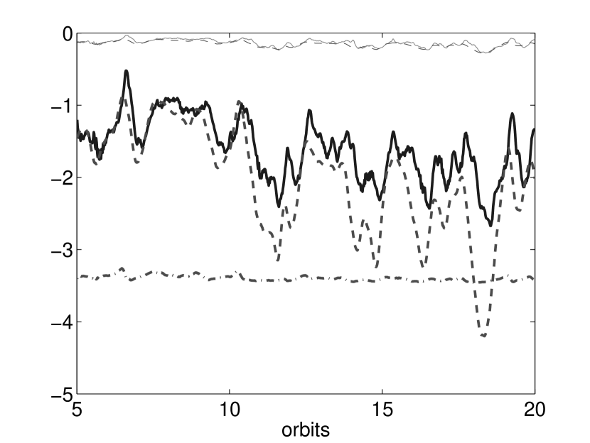
Figure 3: Volume averaged pressure anisotropy ($4\pi\Delta p/B^{2}$; $\Delta p=p_{\parallel}-p_{\perp}$) for electrons (thin solid line) and ions (thick solid line), compared to the anisotropy thresholds for the ion cyclotron (thick dashed line), mirror (thick dot-dashed line), and electron whistler (thin dashed line) instabilities. The ion to electron temperature ratio is set to $10$ after the initial saturation of the MRI at 5 orbits.

The magnitude of the viscous heating in equation (5) is directly proportional to the pressure anisotropy $\Delta p_{s}$, which is $<0$ on average and saturates at a value close to the $p_{\perp,s}>p_{\parallel,s}$ thresholds discussed above (as shown explicitly in Fig. 3 discussed in the next section). For an analytic estimate, we assume that the ion and electron pressure anisotropies are bounded by the ion cyclotron and whistler thresholds, respectively. We then estimate the viscous heating of electrons and ions in the collisionless limit using equations (5), (10), and (11)

$$q_{V,s}^{+}\propto S_{s}\beta_{s}^{1-\alpha_{s}}.$$ (13)

The ion cyclotron and whistler thresholds correspond to $S_{i}/S_{e}\approx 3$ and $\alpha_{i}\approx\alpha_{e}\approx 0.5$, in which case $q_{V,s}^{+}\propto T_{s}^{1/2}$. Viscous heating in a collisionless plasma is thus quite different from that in a collisional plasma: the electron and ion heating rates are comparable when $T_{e}\sim T_{i}$. Indeed, in the absence of radiative cooling, equations (13) and (5) imply that the electron to ion temperature ratio approaches $T_{e}/T_{i}\sim(S_{e}/S_{i})^{2}\sim 0.1$ at late times, if viscous heating is the dominant heating mechanism (even if the ions are initially much hotter than the electrons).

3 Numerical Simulations

In our previous work (SHQS) we modified the ZEUS MHD code (Stone & Norman, 1992a, b) to model the dynamics of the MRI in a collisionless plasma, by including pressure anisotropy, thermal conduction along field lines, and subgrid models for pitch angle scattering by microinstabilities when the pressure anisotropy exceeds the thresholds (discussed in §2.2.1). Our previous work modeled a single fluid, effectively the ions since they typically dominate the pressure if $T_{i}\gg T_{e}$. We now extend this work to include both ions and electrons. As in SHQS, we restrict ourselves to local shearing box simulations.

We solve the mass and momentum conservation equations for the shearing box in MHD (eqs. [35] and [36] in SHQS), where the pressure is the sum of electron and ion pressures, each evolved according to equations (1) and (2). Heat fluxes parallel to the field lines (${\bf q_{\perp}}$ and $\bf q_{\bf\parallel}$) are given by equations (40)-(44) of SHQS applied to electrons and ions. The conductivity along the field lines is given approximately by $\kappa\sim v_{th}^{2}/(v_{th}k_{L}+\nu_{eff})$ where $v_{th}$ is the thermal velocity of the species, $\nu_{eff}$ is the pitch angle scattering rate due the microinstabilities, and $k_{L}$ is a parameter that corresponds to the typical wavenumber for Landau damping; this gives the correct collisionless damping rate for a fluctuation whose wavenumber is $k_{L}$ but is only approximate for other modes (Sharma, 2006). For small $\nu_{eff}$, the conductivity in the heat flux is $\propto k_{L}^{-1}$ so that small values of $k_{L}$ correspond to rapid heat conduction while $k_{L}\rightarrow\infty$ is the adiabatic (CGL) limit with no heat conduction.

In our simulations, the usual shearing box boundary conditions are used (Hawley, Gammie, & Balbus 1995). Initial conditions are described in SHQS. The present simulations use a purely vertical initial field with $\beta=400$. In all runs we initiate a specified electron and ion temperature ratio at the end of 5 orbits so that our results are not affected by the strong channel phase at $\sim 4$ orbits that represents the initial non-linear saturation of the MRI. Electron and ion cooling is neglected. Unless specified otherwise, the resolution is $N_{x}\times N_{y}\times N_{z}=27\times 59\times 27$, and the box size $L_{x}\times L_{y}\times L_{z}=1\times 2\pi\times 1$. The initial parameters in code units are: ion pressure $p_{0}=10^{-6}$, rotation rate $\Omega=10^{-3}$, and initial density $\rho=1$ (as in SHQS). The thermal conduction parameter $k_{L}=0.5/\delta z$ for both electrons and ions, where $\delta z~{}(=L_{z}/N_{z})$ is the grid spacing in the vertical direction. Note that this value of the conductivity corresponds to correctly capturing Landau damping for modes with wavelengths of $(4\pi/N_{z})L_{z}\approx 0.5L_{z}$, i.e., for modes whose wavelengths are approximately half the size of the box.

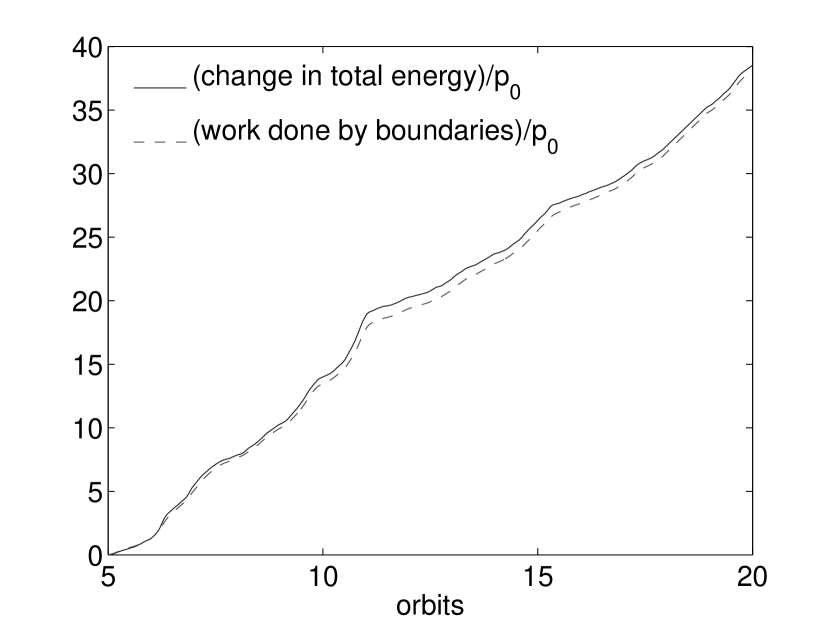
Figure 1: The increase in total energy normalized to the initial pressure $p_{0}$ (solid line) in shearing box simulations of the MRI, compared to the work done by the stresses at the boundaries (dashed line). For a conservative calculation these two curves would agree identically. This is not the case because ZEUS is non-conservative. Nonetheless, our method of improving energy conservation in ZEUS (based on Turner et al., 2003) conserves energy to better than $\sim 5\%$ over 15 orbits.

Since ZEUS is not a conservative code, energy is lost because of numerical dissipation. However, to quantify the importance of different heating mechanisms it is desirable to quantitatively track the energetics of the accretion flow. To do so, we have implemented the method of Turner et al. (2003) in which energy conservation in ZEUS is significantly improved by keeping track of the kinetic and magnetic energies lost because of grid-scale averaging. This energy can also, if desired, be added as a source of plasma heating. However, we do not do so because it is physically unclear which species should receive this energy. In what follows we identify energy lost numerically in the magnetic field update as “numerical resistive” heating ($q^{+}_{NR}$) and energy lost in the transport step for momentum as “numerical viscous” ($q^{+}_{NV}$) heating. Compressive heating, $-p_{\perp}{\bf\nabla\cdot V}$, is negligible because the MRI is relatively incompressible. In addition to numerical heating due to grid-scale dissipation, there is also viscous heating at large-scales due to pressure anisotropy ($q^{+}_{V}$; see eq. [5]). This is captured by our simulations—including the correct ratio of electron to ion heating—and represents direct conversion of gravitational potential energy into heat at large scales (see §2). Figure 1 shows a plot comparing the change in the total plasma energy with the work done by the boundaries in a typical shearing box simulation. Energy is conserved to within $3\times 10^{-3}$ over a disk rotation period, which is adequate for our purposes.

3.1 Stresses and heating rates

Tables 1 & 2 summarize the properties of a number of simulations with the ion to electron temperature ratio initialized at values from $1-10^{4}$ after the MRI saturates at 5 orbits. We find that the properties of saturated MRI turbulence in a collisionless plasma are relatively insensitive (to within a factor of few) to the conductivity (parameterized by $k_{L}$) or numerical resolution. In particular, angular momentum transport quantities like the anisotropic stress ($\alpha_{A}$, where $\alpha$ is the stress divided by the initial pressure), Maxwell stress ($\alpha_{M}$), and Reynolds stress ($\alpha_{R}$), and the associated viscous ($q_{V}^{+}$), “numerical resistive” ($q^{+}_{NR}$), and “numerical viscous” ($q^{+}_{NV}$) heating rates do not depend sensitively on $k_{L}$ or resolution. Instead, the most important physical effect in the evolution of the MRI in a collisionless plasma is pitch angle scattering by kinetic instabilities (§2.2.1), which determines the magnitude of the anisotropic stress and thus the magnitude of the viscous heating. For the pitch angle scattering thresholds described in §2.2.1 we find that anisotropic stress and the associated viscous heating are the dominant terms in the angular momentum and internal energy equations. In addition, viscous heating is dominated by direct heating via the large-scale shear (eq. [6]; $q^{+}_{V1}$); heating due to the turbulent fluctuations (eq. [7]; $q^{+}_{V2}$) is significantly smaller (see Tables 1 & 2).

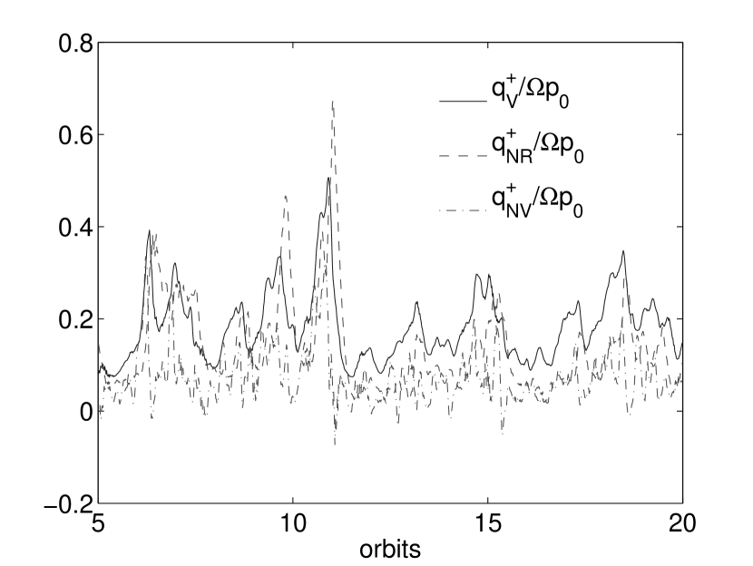
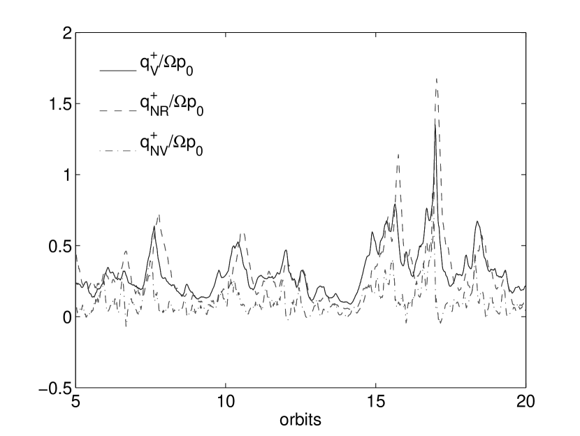
Figure 2: Different contributions to plasma heating in shearing box simulations of the MRI for initially cold electrons ($T_{i}/T_{e}=10^{4}$ at 5 orbits). Left: resolution of $27\times 59\times 27$ resolution with $k_{L}=0.5/\delta z$, Right: resolution of $54\times 118\times 54$ with $k_{L}=0.25/\delta z$. $q_{V}^{+}$ is the heating due to anisotropic viscosity at large scales (electron + ion, but primarily ion because $T_{i}\gg T_{e}$); $q_{NR}^{+}$, the numerical loss of magnetic energy; $q_{NV}^{+}$, the numerical loss of kinetic energy. Viscous heating ($q_{V}^{+}$) accounts for $\sim 50\%$ of the heating in our simulations.

Figure 2 shows the volume average of different heating rates as a function of time in our shearing box simulations with $T_{i}/T_{e}=10^{4}$ at 5 orbits, for $N_{x}\times N_{y}\times N_{z}=27\times 59\times 27$ and $k_{L}=0.5/\delta z$ (left), and $N_{x}\times N_{y}\times N_{z}=54\times 118\times 54$ and $k_{L}=0.25/\delta z$ (right). These combinations of resolution and $k_{L}$ correspond to the same conductivity in the two different simulations. Both the high and low resolution simulations show statistically similar heating results. Direct viscous heating is slightly larger than numerical resistivity and viscosity, implying that $\sim 50\%$ of the gravitational potential energy of the accretion flow is directly converted into heat at large scales (see also Table 1). Figure 2 also shows that the different heating rates are correlated and fluctuate together in time. Although the viscous heating rate varies as a function of time, we find that the ratio of the ion to the electron viscous heating does not show as large statistical variations, i.e., the ion and electron heating rates increase/decrease together in tandem.

Figure 3 shows the volume averaged pressure anisotropy for electrons and ions with $T_{i}/T_{e}$ set to 10 at the end of 5 orbits; the mirror, ion cyclotron, and electron whistler thresholds are also shown. The ion pressure anisotropy is larger than that of the electrons for two reasons: first, the electron pressure anisotropy threshold is smaller than that of the ions ($S_{e}\sim 0.4S_{i}$), and second, the electron $\beta$ is smaller by a factor of 10. Figure 3 also shows that the electron pressure anisotropy is relatively close to the electron whistler instability threshold and that the ion pressure anisotropy roughly tracks the ion cyclotron threshold.

In a collisionless plasma, the MRI grows faster for an initial magnetic field configuration with $B_{\phi}=B_{z}$ than for $B_{\phi}=0$ (Quataert, Dorland, & Hammett 2002; Sharma, Hammett, & Quataert 2003). However, the nonlinear saturated state is similar to that of the pure vertical field case described here (Sharma, 2006). In particular, the anisotropic stress is again comparable to the Maxwell stress and viscous heating accounts for a significant fraction of the total heating of the plasma.

To quantify the relative heating of ions and electrons as a function of $T_{i}/T_{e}$, we initialize simulations in the saturated turbulent state (after 5 orbits) with $T_{i}/T_{e}=10^{4},10^{3},10^{2},10,$ & $1$. Figure 4 shows the ratio of the volume averaged ion and electron temperatures for $k_{L}=0.5/\delta z$, and in the CGL limit ($q_{\perp}=q_{\parallel}=0$). Initially cold electrons become heated significantly by viscous heating as discussed in §2.2. Based on extrapolating the result of Figure 4 to even later times, we estimate that the late-time value of $T_{i}/T_{e}$ due to viscous heating alone is $\approx 10-30$, in reasonable agreement with the analytic estimate in §2.2.

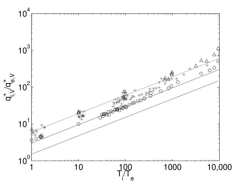
Figure 5: The ion to electron heating ratio as a function of the temperature ratio for: $k_{L}=0.5/\delta z$, resolution $27\times 59\times 27$ (+); $k_{L}=0.25/\delta z$, resolution $54\times 118\times 54$ ($\triangle$); and the CGL limit, resolution $27\times 59\times 27$ (o). The ion to electron heating ratio is slightly larger (less than a factor of 2) with thermal conduction. The results with double the resolution are comparable to the standard resolution showing that the results are reasonably converged. The three solid lines correspond to $q^{+}_{i}/q^{+}_{e}=$ 6 $(T_{i}/T_{e})^{1/2}$, 3 $(T_{i}/T_{e})^{1/2}$, and 1.5 $(T_{i}/T_{e})^{1/2}$ (from top to bottom). These estimates of the electron heating rate, based on our analytic prediction from §2.2, approximate the numerical simulations reasonably well; they are used to calculate the radiative efficiency in §4 and Figure 6. For this plot, the heating and temperature ratios are averaged over 0.1 orbits in a number of simulations (so that $T_{i}/T_{e}$ is roughly constant over the averaging).

Figure 5 shows the ratio of the volume averaged ion and electron heating rates as a function of $T_{i}/T_{e}$ for the same calculations as in Figure 4 (‘o’ for CGL, ‘$+$’ for $k_{L}=0.5/\delta z$, and ‘$\triangle$’ for a higher resolution simulations with $k_{L}=0.25/\delta z$). This plot was made by averaging the heating and $T_{i}/T_{e}$ over 0.1 orbits in a number of different simulations (so that the temperature ratio is fairly constant over the time of averaging). The middle solid line in Figure 5 shows $q^{+}_{V,i}/q^{+}_{V,e}=3(T_{i}/T_{e})^{1/2}$, which is roughly the analytic prediction from §2.2 (eq. [13]) assuming that the ion and electron pressure anisotropies are set by the ion cyclotron and whistler instabilities, respectively. The agreement between the analytic prediction and the numerical results is particularly good in the absence of conduction: the heating ratio $q^{+}_{V,i}/q^{+}_{V,e}$ is slightly larger (less than a factor of two) with conduction than without it. Figure 5 also shows that the electron to ion heating ratio does not depend sensitively on the resolution of the simulation.

4 Implications

To quantify the importance of viscous heating for observations of accreting black holes, we use a heating prescription motivated by our analytic and numerical results in one-dimensional models of RIAFs (based on Quataert & Narayan 1999). From equation (13) and Figure 5, we approximate the fraction of the viscous energy that heats the electrons as $\delta\equiv q_{e}^{+}/q_{i}^{+}\approx 0.33(T_{e}/T_{i})^{1/2}$. This approximation is consistent with our numerical simulations in the CGL limit; $\delta$ is slightly smaller if thermal conduction is included (Fig. 5). Our one-dimensional calculations include electron cooling by free-free emission, synchrotron radiation, and Inverse Compton emission. The electron temperature, the spectrum of radiation, and the radiative efficiency are calculated self-consistently given the assumed electron heating rate and the density, radial velocity, etc. from a one-dimensional dynamical model. For more details, see Quataert & Narayan (1999) and references therein.

Figure 6 shows the resulting radiative efficiency of RIAF models as a function of accretion rate; we assumed $\alpha=0.1$ and $\beta=10$ in these calculations but the results are not that sensitive to reasonable variations in these parameters. Three choices of $\delta$ ($\delta=0.66[T_{e}/T_{i}]^{1/2}$, $\delta=0.33[T_{e}/T_{i}]^{1/2}$, and $\delta=0.17[T_{e}/T_{i}]^{1/2}$ ) are shown, given the uncertainty in the exact magnitude of the viscous heating (e.g., the relative contribution of viscous heating and other heating mechanisms, the effects of thermal conduction, and the uncertainty in the pressure anisotropy thresholds). For concreteness, the calculations shown in Figure 6 assume that the accretion rate is constant with radius. Since most of the radiation is produced at small radii, the radiative efficiency only depends on the accretion rate at $\sim 10$ Schwarzschild radii and so the x-axis in Figure 6 can be interpreted as such. Figure 6 demonstrates that with analytically and numerically motivated viscous heating rates, the radiative efficiency is $\gtrsim 0.5\%$ for $\dot{M}\gtrsim 10^{-4}\,\dot{M}_{\rm Edd}$ for all of our electron heating models considered. At very low $\dot{M}$, the efficiency decreases in all models because the electron cooling time (primarily by synchrotron radiation) becomes longer than the inflow time in the accretion flow. Since our calculations in Figure 6 do not account for the $\sim 50\%$ of the gravitational potential energy lost via grid-scale averaging in our shearing box simulations (see §3), the resulting radiative efficiencies are likely a lower limit to the true radiative efficiency.

4.1 Electron collisionality

One possible caveat to the application of our fully collisionless results to RIAF models is that if the electron Coulomb collision frequency $\nu_{e}$ is significantly larger than the rate at which pressure anisotropy is created by turbulence, then Coulomb collisions will suppress the electron pressure anisotropy faster than kinetic instabilities. As a result, electron heating by anisotropic pressure will be negligible. We thus estimate an upper limit on the mass accretion rate above which collisions will be able to wipe out the pressure anisotropy. This calculation is analogous to standard estimates in the literature of the critical mass accretion rate $\sim\alpha^{2}\dot{M}_{\rm Edd}$ above which it is not possible to maintain a two-temperature RIAF because Coulomb collisions thermally couple the electrons and protons on an inflow time (Rees et. al., 1982). Because electron pitch angle scattering is $\sim m_{p}/m_{e}\sim 10^{3}$ faster than electron-proton energy exchange, the critical accretion rate above which the electrons are isotropized might be expected to be $\sim 10^{-3}\alpha^{2}\dot{M}_{\rm Edd}$. This result is not correct, however, for two reasons: 1. Pressure anisotropy is created on a timescale even shorter than an eddy turnover time due to the fluctuating magnetic field, rather than on the inflow time (see eq. [15] discussed below). 2. The electron Coulomb collision frequency depends strongly on electron temperature, which is itself a strong function of accretion rate.

The average pressure anisotropy can be estimated from equation (4). The second term vanishes after spatial averaging. Assuming that fluctuations are incompressible, and neglecting the heat fluxes, the dominant terms are

$$\frac{\partial}{\partial t}\Delta p_{e}\sim-3p_{e}{\bf\hat{b}\hat{b}:\nabla V}-\nu_{eff,e}\Delta p_{e}-\nu_{e}\Delta p_{e}$$ (14)

where we have added a separate term for the rate $\nu_{e}$ of pitch angle scattering by Coulomb collisions to clearly distinguish between the effects of Coulomb collisions and microinstabilities ($\nu_{eff,e}$). If $\nu_{e}$ is negligible, then steady state occurs when the pitch angle scattering caused by microinstabilities, at the rate $\nu_{eff,e}$ balances the first term on the RHS of equation (14). The scattering by microinstabilities occurs very rapidly (on the electron cyclotron timescales) if the pressure anisotropy is larger than the threshold to excite the instabilities, so in practice $\nu_{eff,e}$ will always be just large enough to keep $\Delta p_{e}$ near the threshold. Thus balancing the first and second terms on the RHS gives

$$\nu_{eff,e}\sim 3\frac{p_{e}}{\Delta p_{e}}{\bf\hat{b}\hat{b}:\nabla V}\sim 35\Omega\beta^{1/2}\left(\frac{T_{e}}{T_{i}}\right)^{1/2},$$ (15)

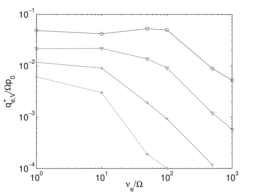
Figure 7: Electron heating rate (volume averaged from 5 to 20 orbits) due to anisotropic viscosity as a function of the electron collisionality for simulations with no heat conduction ($k_{L}\rightarrow\infty$). The ion to electron temperature ratio is initialized to $10^{3}$ ($*$), $10^{2}$ (+), 10 ($\triangledown$), & $1$ (o) after 5 orbits. Viscous heating of electrons is suppressed at high electron collisionality (high $\nu_{e}$); the critical value of $\nu_{e}/\Omega$ in the numerical calculations is in reasonable agreement with the analytic estimate in equation (15).

using $\alpha_{e}$ and $S_{e}$ from §2.2.1. If the collisional pitch angle scattering rate exceeds that estimated in equation (15), then electron viscous heating will be reduced relative to the pure collisionless calculations presented in §2 & 3. Figure 7 shows this explicitly by plotting the average electron heating rate for shearing-box simulations that include an additional Coulomb collision rate $\nu_{e}$, in addition to the subgrid models for kinetic instabilities.  The numerical results in Figure 7 show that above a critical $\nu_{e}$,  electron viscous heating is substantially reduced; this critical $\nu_{e}$ depends on $T_{e}/T_{i}$, in good agreement with the analytic estimate in equation (15).

To apply the above results to RIAF models, we note that for the accretion rates of interest, the electrons are only marginally relativistic (see Fig. 8 discussed below) and so we use the Coulomb collision frequency for non-relativistic electrons. Using the ADAF solution of Narayan & Yi (1995) to estimate the density and ion temperature in the accretion flow, we find that electron Coulomb collisions are negligible for the isotropization of the electron pressure for accretion rates satisfying

$${\dot{M}\over\dot{M}_{\rm Edd}}\ll 0.06\left(\frac{\alpha}{0.1}\right)\left(\frac{\beta}{10}\right)^{1/2}\left(\frac{r}{10}\right)^{1/2}\theta_{e}^{2},$$ (16)

where $r$ is the distance from the central object in units of the Schwarzschild radius and $\theta_{e}=kT_{e}/m_{e}c^{2}$ is the electron temperature normalized to the electron rest mass energy.

Figure 8 shows the electron temperature as a function of radius for our one-dimensional RIAF models with $\delta=0.33(T_{e}/T_{i})^{1/2}$, for a variety of accretion rates (solid lines). The protons are at roughly the virial temperature for all $\dot{M}$ since they do not cool significantly. By contrast, the electron temperature depends strongly on $\dot{M}$, with the temperature decreasing at small radii for increasing $\dot{M}$. For $\dot{M}\lesssim 10^{-5}\dot{M}_{\rm Edd}$, however, the electron temperature is relatively independent of $\dot{M}$ because the electron cooling time becomes long compared to the inflow time. The dotted line shows the electron temperature for low $\dot{M}$ for $\delta=0.66(T_{e}/T_{i})^{1/2}$; the temperature is a factor of $\sim 2$ larger at small radii in this case because of the additional heating.

Figure 8 shows that $\theta_{e}\sim 1$ at $\dot{M}\sim 10^{-2}\dot{M}_{\rm Edd}$; at this high $\dot{M}$, the electron temperature is relatively independent of our assumptions about the electron heating. This is because the electrons are efficiently cooled by synchrotron radiation and Inverse Compton emission, and become marginally relativistic. Using $\theta_{e}\sim 1$ in equation (16), we conclude that electron Coulomb collisions are unimportant for isotropizing the electrons for $\dot{M}\ll 0.06\dot{M}_{\rm Edd}$. Since the electron temperature increases with decreasing $\dot{M}$ (Fig. 8), Coulomb collisions rapidly become unimportant for isotropizing the electrons below $\sim 0.06\dot{M}_{\rm Edd}$. We thus conclude that the collisionless calculations of the radiative efficiency in Figure 6 should be applicable for essentially all of the accretion rates considered.

5 Discussion

We have shown that viscosity arising from anisotropic pressure is a significant source of heating in hot accretion flows (RIAFs). In shearing box simulations of the MRI in collisionless plasmas, viscous heating is comparable to the rate at which energy is lost by grid-scale numerical averaging. It thus accounts for $\sim 50\%$ of the gravitational potential energy released by the inflowing matter. In a real accretion disk, the fate of the remaining $\sim 50\%$ of the energy that is dissipated at small scales is unclear. Although viscosity along the field lines due to pressure anisotropy can damp parallel motions, it cannot dissipate energy in motions perpendicular to the field lines (e.g., Alfvén modes). This energy is presumably dissipated through collisionless damping of fluctuations in a turbulent cascade at the ion Larmor radius (Quataert, 1998; Howes et al., 2006).

In contrast to the kinetic and magnetic energy lost to grid-scale averaging, the physics of viscous heating at large scales is well-captured by MRI simulations and can be accurately approximated using a simple analytic expression that depends primarily on the average pressure anisotropy in the plasma (eq. [13]). In turn, the magnitude of the pressure anisotropy is set by pitch angle scattering due to small-scale kinetic instabilities (see §2.2.1). We thus conclude that pressure anisotropy plays an essential role in both the energy (via viscous heating) and angular momentum (via anisotropic stress) budgets of RIAFs. This interplay of pressure anisotropy and microinstabilities is likely to be important in many other weakly collisional plasmas, e.g., the solar wind and X-ray clusters (e.g., Schekochihin et al., 2005). The only way out of this conclusion is if there is efficient generation of high frequency fluctuations that provide pitch angle scattering (and thus pressure isotropization) at a rate much faster than that of the kinetic instabilities discussed in §2.2.1. This does not appear to be true in the solar wind, where large pressure anisotropies are measured (e.g., Cranmer et al., 1999) and where there is in situ experimental evidence for pressure isotropization via the firehose instability (Kasper, Lazarus, & Gary, 2002).

In addition to viscous heating, numerical simulations can in principle also capture heating by the collisionless (Landau/Barnes) damping of large-scale turbulent fluctuations. In particular, the slow magnetosonic mode is strongly damped in a collisionless plasma even on large scales and has been proposed as a source of proton heating in RIAFs (e.g., Quataert, 1998; Blackman, 1999). We find little direct evidence for such heating in our numerical simulations; the part of the anisotropic pressure heating (eq. [5]) proportional to the background shear $d\Omega/d\ln r$ (eq. [6]) dominates over the part proportional to the turbulent velocity fluctuations (eq. [7]) for all of our simulations (see Table 1). In addition, the relatively weak dependence of the plasma heating on the Landau damping parameter $k_{L}$ (see Tables 1 & 2) suggests that very little of the turbulent energy is dissipated via collisionless damping at large scales. In fact, even in the limit of zero conductivity ($k_{L}\rightarrow\infty$) and thus no collisionless damping (the double-adiabatic limit) we find roughly the same energetics in our shearing box simulations. These results imply that heating due to work done by anisotropic stress dominates collisionless damping on large scales in RIAFs. Collisionless damping may become important on smaller scales (that we cannot resolve) where the turbulence can be better approximated as a superposition of linear modes (on large scales the fluctuating magnetic field is much larger than the mean field). Indeed, with higher resolution it may turn out that instead of being lost to grid-scale averaging, most of the kinetic and magnetic energy is damped via collisionless damping at intermediate scales. In addition, more accurate fully kinetic treatments may be needed to quantify the heating by collisionless damping on large scales in MRI simulations.

Our results on viscous heating imply radiative efficiencies of $\gtrsim 0.5\%$ for $\dot{M}\gtrsim 10^{-4}\dot{M}_{Edd}$ (Fig. 6). With such significant radiative efficiencies, the low luminosities of many accreting black holes can only be understood if most of the mass supplied to the flow at large radii does not reach the central object. Our results are thus consistent with global numerical simulations of magnetized RIAFs, which show that only a small fraction of mass is actually accreted (e.g., Stone & Pringle 2001; Hawley, Balbus, & Stone 2001).

To give a concrete example of the implications of our results, the Bondi accretion rate for Sgr A* in the Galactic Center is estimated to be $\sim 3\times 10^{-6}-10^{-5}M_{\odot}\,{\rm yr^{-1}}$ (e.g., Quataert, 2004; Cuadra et al., 2006), which corresponds to $\dot{M}/\dot{M}_{\rm Edd}\sim 10^{-4}$. Our results predict a radiative efficiency of $\approx 0.005-0.03$ for this $\dot{M}$, with the uncertainty in the radiative efficiency arising from uncertainties in the exact rate of electron viscous heating. If gas were to accrete at the Bondi rate, a radiative efficiency of $0.01$ implies a luminosity $\sim 10^{3}$ times larger than what is observed from Sgr A*, implying that the accretion rate must be well below the Bondi rate. Requiring $L\approx 10^{36}$ ergs s^-1 as is observed, our predicted radiative efficiencies (Fig. 6) imply an accretion rate of $\dot{M}\approx 10^{-7}-10^{-8}\,{\rm M_{\odot}\,yr^{-1}}$ where the range accounts for the range of radiative efficiencies in Figure 6. Measurements of the rotation measure from Sgr A* are consistent with such a low accretion rate (Marrone et al., 2007). In addition, VLBI interferometry of Sgr A* finds a size of $\approx 15R_{S}$ at 100 GHz (Bower et al., 2004, 2006). The corresponding brightness temperature is $\approx 3\times 10^{10}$ K. At low $\dot{M}$, our models for the electron temperature at $\approx 15R_{S}$ are in reasonable agreement with this result (Fig. 8).

Table 1: Heating Diagnostics for Simulations with initially Cold Electrons ($T_{i}/T_{e}=10^{4}$ at 5 orbits)

$k_{L}$	$N_{x}\times N_{y}\times N_{z}$	$\alpha_{A}$	$\alpha_{M}$	$\alpha_{R}$	$q_{V1}^{+}/\Omega p_{0}$	$q_{V2}^{+}/\Omega p_{0}$	$q_{NR}^{+}/\Omega p_{0}$	$q_{NV}^{+}/\Omega p_{0}$
$0.5/\delta z$	$27\times 59\times 27$	0.12	0.097	0.048	0.18	0.049	0.14	0.074
$0.5/\delta z$	$54\times 118\times 54$	0.21	0.26	0.083	0.31	0.06	0.38	0.13
$0.25/\delta z$	$54\times 118\times 54$	0.18	0.21	0.073	0.27	0.043	0.3	0.11
$0.125/\delta z$	$27\times 59\times 27$	0.16	0.21	0.084	0.25	0.04	0.32	0.13
$0.125/\delta z$	$54\times 118\times 54$	0.15	0.20	0.060	0.23	0.049	0.31	0.094
$2/\delta z$	$27\times 59\times 27$	0.16	0.15	0.073	0.23	0.016	0.22	0.11
$2/\delta z$	$54\times 118\times 54$	0.19	0.22	0.071	0.28	0.039	0.30	0.11
$\infty$	$27\times 59\times 27$	0.19	0.20	0.086	0.27	0.013	0.25	0.13
$\infty$	$54\times 118\times 54$	0.18	0.22	0.067	0.27	0.026	0.27	0.1

Table 2: Heating Diagnostics for Different $T_{i}/T_{e}$

$T_{i}/T_{e}$	$k_{L}$	$\alpha_{A}$	$\alpha_{M}$	$\alpha_{R}$	$q_{V1,i}^{+}/\Omega p_{0}$	$q_{V2,i}^{+}/\Omega p_{0}$	$q_{V1,e}^{+}/\Omega p_{0}$	$q_{V2,e}^{+}/\Omega p_{0}$	$q_{NR}^{+}/\Omega p_{0}$	$q_{NV}^{+}/\Omega p_{0}$
1000	$0.5/\delta z$	0.16	0.17	0.077	0.16	0.0037	$5.9\times 10^{-4}$	$1.6\times 10^{-4}$	0.26	0.12
1000	$\infty$	0.15	0.13	0.065	0.16	-0.0014	$8.2\times 10^{-4}$	$2.9\times 10^{-4}$	0.17	0.1
100	$0.5/\delta z$	0.13	0.11	0.057	0.16	0.0039	0.003	$3.1\times 10^{-4}$	0.17	0.088
100	$\infty$	0.18	0.17	0.079	0.16	-0.0024	0.0042	$6.9\times 10^{-4}$	0.23	0.12
10	$0.5/\delta z$	0.16	0.15	0.071	0.16	0.0027	0.01	$3.7\times 10^{-4}$	0.23	0.11
10	$\infty$	0.15	0.12	0.061	0.16	-0.0055	0.014	0.0012	0.16	0.09
1	$0.5/\delta z$	0.17	0.13	0.07	0.16	-0.0015	0.03	$2.1\times 10^{-4}$	0.2	0.11
1	$\infty$	0.18	0.13	0.068	0.16	-0.018	0.035	0.0056	0.17	0.1

Figure 6: Radiative efficiency as a function of mass accretion rate in one dimensional models of RIAFs (based on the calculations described in Quataert & Narayan 1999). These models assume $\alpha=0.1$ and $\beta=10$ in determining the density and magnetic field strength in the accretion flow. Since most of the radiation is produced close to the black hole, $\dot{M}$ can be interpreted as the accretion rate in the inner $\sim 10R_{S}$. The solid line corresponds to $\delta\equiv q^{+}_{e}/q^{+}_{i}=0.33(T_{e}/T_{i})^{1/2}$, and the dashed lines to $\delta=0.66(T_{e}/T_{i})^{1/2}$ (upper) and $\delta=0.17(T_{e}/T_{i})^{1/2}$ (lower). At high $\dot{M}$, Coulomb collisions transfer energy from the ions to the electrons and so the radiative efficiency becomes relatively independent of the assumptions regarding $\delta$. At very low $\dot{M}$, the electron cooling time is longer than the inflow time and the radiative efficiency decreases in all models.

Figure 8: Electron temperature as a function of radius for our one-dimensional RIAF models with $\alpha=0.1$, $\beta=10$, and $\delta=0.33(T_{e}/T_{i})^{1/2}$. The solid lines correspond to $\log[\dot{M}/\dot{M}_{\rm Edd}]=$ -2, -2.5, -3, -3.5, -4, -4.5, -5, -5.5, -6 (from bottom to top). The electron temperature is independent of $\dot{M}$ for even lower accretion rates. The dotted line shows the electron temperature for $\delta=0.66(T_{e}/T_{i})^{1/2}$ and $\log[\dot{M}/\dot{M}_{\rm Edd}]=-6$. To demonstrate that at high $\dot{M}$ the electron temperature is relatively independent of our model assumptions, the dashed line shows $T_{e}(r)$ for $\dot{M}=10^{-2}\dot{M}_{\rm Edd}$ and $\delta=10^{-3}$, while the dot-dashed line is for $\dot{M}=10^{-2}\dot{M}_{\rm Edd}$ and $\delta=0.66(T_{e}/T_{i})^{1/2}$.

References

- Armitage (1998) Armitage, P. J. 1998, ApJ, 501, L189
- Balbus & Hawley (1991) Balbus, S. A. & Hawley, J. F. 1991 , ApJ, 376, 214
- Balbus & Hawley (1998) Balbus, S. A. & Hawley, J. F. 1998 , Rev.Mod.Phys., 70, 1
- Balbus (2004) Balbus, S. A. 2004, ApJ, 616, 857
- Bisnovatyi-Kogan & Lovelace (1997) Bisnovatyi-Kogan, G. S. & Lovelace, R. V. E. 1997, 486, L43
- Blackman (1999) Blackman, E. G. 1999, MNRAS, 302, 723
- Blandford & Begelman (1999) Blandford, R. D. & Begelman, M. C. 1999, MNRAS, 303, L1
- Bower et al. (2004) Bower, G. C., Falcke, H., Herrnstein, R. M., Zhao, J., Goss, W., & Backer, D. C. 2004, Science, 304, 704
- Bower et al. (2006) Bower, G. C., Goss, W. M., Falcke, H., Backer, D. C., & Lithwick, Y. 2006, ApJ, 648, L127
- Braginskii (1965) Braginskii, S. I. 1965, Reviews of Plasma Physics, Vol. 1, Consultants Bureau, 1965
- Budker (1961) Budker, G. I. 1961, Plasma Physics and the Problem of Controlled Thermonuclear Reactions, Vol. 1, M. A. Leontovich, Pergamon Press, New York
- Chew, Glodberger, & Low (1956) Chew, C. F., Goldberger, M. L., & Low, F. E. 1956, Proc. R. Soc. London, Ser. A, 236, 112
- Cranmer et al. (1999) Cranmer, S. R. et al. 1999, ApJ, 511, 481
- Cuadra et al. (2006) Cuadra, J., Nayashkin, S., Springer, V., & Di Matteo, T. 2006, MNRAS, 366, 358
- Fabian & Canizares (1988) Fabian, A. C. & Canizares, C. R. 1988, Nature, 333, 829
- Fabian & Rees (1995) Fabian, A. C. & Rees, M. J. 1995, MNRAS, 277, 55
- Gary & Lee (1994) Gary, S. P., Lee, M. A. 1994, J. Geophys. Res., 99, 11297
- Gary & Wang (1996) Gary, S. P., Wang, J. 1996, J. Geophys. Res., 101, 10749
- Gary et al. (1998) Gary, S. P., Hui, L., O’Rourke, S., & Winske, D. 1998, J. Geophys. Res., 103, 14567
- Goldreich & Sridhar (1995) Goldreich, P. & Sridhar, S. 1995, ApJ, 438, 763
- Gruzinov (1998) Gruzinov, A. V. 1998, ApJ, 501, 787
- Hasegawa (1969) Hasegawa, A. 1969, Phys. Fluids, 12, 2642
- Hawley, Gammie, & Balbus (1995) Hawley, J. F., Gammie, C. F., & Balbus, S. A. 1995, ApJ, 440, 742
- Hawley, Balbus, & Stone (2001) Hawley, J. F., Balbus, S. A., & Stone, J. M. 2001, ApJ, 554, 49
- Howes et al. (2006) Howes, G. G., Cowley, S. C., Dorland, W., Hammett, G. W., Quataert, E., & Schekochihin, A. A. 2006, ApJ, 651, 590
- Ichimaru (1977) Ichimaru, S. 1977, ApJ, 214, 840
- Kasper, Lazarus, & Gary (2002) Kasper, J. C., Lazarus, A. J., & Gary, S. P. 2002, Geophys. Res. Lett., 29, 1839
- Krolik & Zweibel (2006) Krolik, J. H. & Zweibel, E. G. 2006, ApJ, 644, 651
- Kulsrud (1983) Kulsrud, R. M. 1983, Handbook of Plasma Physics, M. N. Rosenbluth, & R. Z. Sagdeev, North Holland, New York
- Kulsrud (2005) Kulsrud, R. M. 2005, Plasma Physics for Astrophysics, Princeton University Press, Princeton
- Li & Habbal (2000) Li, X. & Habbal, S. R. 2000, J. Geophys. Res., 105, 27377
- Loewenstein et al. (2001) Loewenstein, M., Mushotzky, R. F., Angelini L., Arnaud, K. A., & Quataert, E. 2001, ApJ, 555, L21
- Marrone et al. (2007) Marrone, D. P., Moran, J. M., Zhao, J., & Rao, R. 2007, ApJ, 654, L57
- McKean, Gary, & Winske (1993) McKean, M. E., Gary, S. P., & Winske, W. D. 1993, J. Geophys. Res., 98, 21313
- Medvedev (2000) Medvedev, M. V. 2000, ApJ, 541, 811
- Narayan & Yi (1995) Narayan, R. & Yi, I. 1995, ApJ, 452, 710
- Narayan, McClintock, & Yi (1996) Narayan, R., McClintock, J. E., & Yi, I. 1996, ApJ, 457, 821
- Narayan, Igumenshchev, & Abramowicz (2000) Narayan, R., Igumenshchev, I. V., Abramowicz, M. A. 2000, 539, 798
- Piontek & Ostriker (2005) Piontek, R. A. & Ostriker, E. C. 2005, ApJ, 629, 849
- Quataert (1998) Quataert, E 1998, ApJ, 500, 978
- Quataert & Narayan (1999) Quataert, E. & Narayan, R. 1999, ApJ, 520, 298
- Quataert & Gruzinov (1999) Quataert, E. & Gruzinov, A. 1999, ApJ, 520, 248
- Quataert & Gruzinov (2000) Quataert, E. & Gruzinov, A. 2000, ApJ, 539, 809
- Quataert, Dorland, & Hammett (2002) Quataert, E., Dorland, W., & Hammett, G. W. 2002, ApJ, 577, 524
- Quataert (2003) Quataert, E. 2003, Astron. Nachr., 324, 435
- Quataert (2004) Quataert, E. 2004, ApJ, 613, 322
- Rees et. al. (1982) Rees, M. J., Phinney, E. S., Begelman, M. C., Blandford, R. D. 1982, Nature, 295, 17
- Rönnmark (1982) Rönnmark, K. 1982, WHAMP—Waves in Homogeneous, Anisotropic, Multicomponent Plasmas, KGI Report No. 179, University of Umeå, Sweden
- Schekochihin et al. (2005) Schekochihin, A. A., Cowley, S. C., Kulsrud, R. M., Hammett, G. W., & Sharma, P. 2005, ApJ, 629, 139
- Shapiro, Lightman, & Eardley (1976) Shapiro, S. L., Lightman, A. P., & Eardley, D. M. 1976, ApJ, 204, 187
- Sharma, Hammett, & Quataert (2003) Sharma, P., Hammett, G. W., & Quataert, E. 2003, ApJ, 596, 1121
- Sharma et al. (2006) Sharma, P., Hammett, G. W., Quataert, E., & J. M. Stone 2006, ApJ, 637, 952
- Sharma (2006) Sharma, P. 2006, Ph.D. thesis, Princeton University, astro-ph/0703542
- Snyder, Hammett, & Dorland (1997) Snyder, P. B., Hammett, G. W. , & Dorland, W. 1997, Phys. Plasmas, 4, 3974
- Stone & Norman (1992a) Stone, J. M., Norman, M. L. 1992a, ApJS, 80, 753
- Stone & Norman (1992b) Stone, J. M., Norman, M. L. 1992b, ApJS, 80, 819
- Stone, Pringle, & Begelman (1999) Stone, J. M., Pringle, J. E., & Begelman, M. C. 1999, MNRAS, 310, 1002
- Stone & Pringle (2001) Stone, J. M. & Pringle, J. E. 2001, MNRAS, 322, 461
- Turner et al. (2003) Turner, N. J., Stone, J. M., Krolik, J. H., & Sano, T. 2003, ApJ, 593, 992
- Winters, Balbus, & Hawley (2003) Winters, W. F., Balbus, S. A., & Hawley, J. F. 2003, ApJ, 589, 543