Cosmological Constraints from SDSS maxBCG Cluster Abundances

Abstract

We perform a maximum likelihood analysis of the cluster abundance measured in the SDSS using the maxBCG cluster finding algorithm. Our analysis is aimed at constraining the power spectrum normalization $\sigma_{8}$, and assumes flat cosmologies with a scale invariant spectrum, massless neutrinos, and CMB and supernova priors $\Omega_{m}h^{2}=0.128\pm 0.01$ and $h=0.72\pm 0.05$ respectively. Following the method described in the companion paper Rozo et al. (2007), we derive $\sigma_{8}=0.92\pm 0.10$ ($1\sigma$) after marginalizing over all major systematic uncertainties. We place strong lower limits on the normalization, $\sigma_{8}>0.76$ ($95\%$ CL) ($>0.68$ at $99\%$ CL). We also find that our analysis favors relatively low values for the slope of the Halo Occupation Distribution (HOD), $\alpha=0.83\pm 0.06$. The uncertainties of these determinations will substantially improve upon completion of an ongoing campaign to estimate dynamical, weak lensing, and X-ray cluster masses in the SDSS maxBCG cluster sample.

1. Introduction

One of the most important problems in observational cosmology today is to resolve the question of whether or not dark energy takes the form of a cosmological constant. While current geometric probes of dark energy such as supernovae and baryon acoustic oscillations unequivocally tell us that dark energy exists, a complementary probe of the dark energy evolution can help us distinguish between a cosmological constant and a dynamical dark energy. The growth of structure is one such probe (Eke et al. 1996; Holder et al. 2001; Evrard et al. 2002; Molnar et al. 2004). In particular, given a geometric probe, an accurate determination of the amplitude of the power spectrum at two different times directly constrains the growth between the two epochs, and can in principle help determine if the dark energy density evolves with redshift. We know the power spectrum amplitude at the time of last scattering with high precision thanks to Cosmic Microwave Background (CMB) experiments (see e.g. Spergel et al. 2006, and references therein), so a precise determination of the current power spectrum normalization may, in principle, distinguish between a dynamical dark energy component and a cosmological constant.

It is well known that the abundance of massive halos in the local universe depends strongly on the amplitude of the matter power spectrum $\sigma_{8}$. In particular, from theoretical considerations (Press & Schechter 1974; Bond et al. 1991; Sheth & Tormen 2002) one expects the number of massive clusters in the universe to be exponentially sensitive to $\sigma_{8}$, a picture that has been confirmed with extensive numerical simulations. Consequently, the number of galaxy clusters within a given survey region ought to be able to provide powerful constraints on $\sigma_{8}$, and, indeed, the literature is rife with these type of studies.

Unfortunately, cluster abundance determinations of $\sigma_{8}$ have to overcome a large variety of difficulties. For instance, the abundance of massive halos in the universe is sensitive not only to $\sigma_{8}$ but also to $\Omega_{m}$, the mean matter density of the universe, which implies that constraints on the number density of massive halos typically result in large degeneracies between $\Omega_{m}$ and $\sigma_{8}$ (though see Rozo et al. 2004). In fact, the main the main obstacle to accurate $\sigma_{8}$ measurements is systematic uncertainties in mass estimates of clusters (see e.g. Pierpaoli et al. 2003; Henry 2004). Consequently, new analyses that properly marginalize over such systematic uncertainties are of particular importance to interpret cluster abundance constraints within a broad cosmological context.

In this work, we use the techniques developed in Rozo et al. (2007) to analyze the Sloan Digital Sky Survey (SDSS) maxBCG cluster sample from Koester et al. (2007a). The analysis of these data uses information from the Rozo et al. (2007) companion paper on the form of the maxBCG selection function, which connects our observable mass proxy — the cluster richness — to halo mass. As discussed in in that work, at this time our understanding of the maxBCG selection function is incomplete, which implies that we have large systematic uncertainties in the selection function. Nevertheless, the large mass range probed by the maxBCG cluster sample allows us to marginalize over these uncertainties and still recover competitive estimates for $\sigma_{8}$, albeit with the inclusion of cosmological priors for $\Omega_{m}h^{2}$ and $h$ in our analysis. Importantly, the results presented in this work ought to be interpreted as an upper limit of how well we can expect $\sigma_{8}$ to be constrained from the current maxBCG cluster sample in the near future. Not only will we soon be able to include additional data such as weak lensing and dynamical cluster mass estimates, but we also expect our understanding of the maxBCG cluster selection function to improve both as an expanded suite of simulations used to calibrate the maxBCG selection function become an even more accurate approximation to reality and as we work towards a more robust richness estimator.

The layout of the paper is as follows. In §2 we briefly describe the maxBCG cluster finding algorithm used to identify the cluster sample analyzed in this work. §3 summarizes the model described in Rozo et al. (2007), including a description of the various parameters and priors used in our analysis. Our cosmological constraints are presented in §4, and discussed in detail in §5.

2. The maxBCG Cluster-Finding Algorithm

Details of how the maxBCG cluster-finding algorithm works can be found in Koester et al. (2007a). Here, we only summarize the main elements of the cluster-finding algorithm.

MaxBCG is an optical cluster-finding algorithm that relies on photometric measurements to overcome projection effects. To detect clusters, maxBCG uses the well known observational fact that galaxy clusters contain a large number of so called ridgeline galaxies: bright, red, early type galaxies that populate a narrow ridgeline in color-magnitude space as a function of redshift. The color distribution of these galaxies is modeled as a narrow Gaussian, while their two dimensional spatial distribution about the cluster center is modeled as a projected Navarro, Frenk, and White (NFW) profile (Navarro et al. 1997). To determine the cluster center, maxBCG relies on the observational fact that, in the vast majority of clusters, there is a clear Brightest Cluster Galaxy (BCG) at or near the center of the cluster. These BCG galaxies tend to be extremely luminous and red, populating the tip of the color-magnitude ridgeline. Their luminosity and colors are also modeled as narrow Gaussians.

Given our model, one can then compute the likelihood that a particular galaxy is the BCG galaxy of a cluster by computing the product ${\cal{L}}_{BCG}{\cal{L}}_{R}$, where ${\cal{L}}_{BCG}(z)$ is the likelihood that the galaxy under consideration has the observed colors and magnitude assuming that it is a BCG at redshift $z$, and ${\cal{L}}_{R}$ is the likelihood that the galaxy distribution around the the candidate BCG will occur under the assumption that the BCG is at the center of cluster (though this is unlikely to be universally true; see e.g. van den Bosch et al. 2005). In computing the ridgeline likelihood ${\cal{L}}_{R}$, only galaxies found within $3\ \mbox{Mpc}$ of the candidate BCG and in a narrow ($3\sigma$) color window around the expected color for ridgeline galaxies at that redshift are considered. The total likelihood ${\cal{L}}={\cal{L}}_{BCG}{\cal{L}}_{R}$ is evaluated at a grid of redshifts, and a photometric redshift estimate for the cluster is obtained by maximizing the likelihood function.

The end result of this process is a likelihood assignment for every galaxy in the survey. The galaxy list is then rank ordered according to likelihood, and the most likely BCG is selected as a BCG. A first rough richness measurement is made by counting the number of galaxies within $1\ \mbox{Mpc}$, which is then used to estimate a characteristic radius for the cluster using the results from Hansen et al. (2005). All ridgeline galaxies above a luminosity cut of $0.4L_{*}$ within this scale radius are considered cluster members, and the number of cluster members is defined as the cluster’s richness, denoted here by $N_{obs}$ and in Koester et al. (2007a) by $N_{gals}^{r_{200}}$ . All BCG candidates within a galaxy overdensity of 200 and within $\Delta z=0.02$ of the cluster just found are dropped from the candidate BCG list. The procedure is then iterated, resulting in a cluster catalog where each cluster has an assigned cluster center, a members’ list, a richness, and a photometric redshift estimate.

3. The Model

In this work, our main observable is the number of clusters within the survey volume as a function of cluster richness, i.e. the richness function. We now summarize the basic picture behind our analysis. A detailed presentation of this formalism can be found in Rozo et al. (2007).

3.1. The Model at a Glance

Suppose we wish an expression for the number of clusters of a given richness. In general, if $P(N_{obs}|m)$ is the probability that a halo of mass $m$ is detected as a cluster with $N_{obs}$ galaxies, the mean density of these clusters is simply

$$\left\langle n\right\rangle=\int dm\ \frac{d\langle\bar{n}\rangle}{dm}P(N_{obs}|m).$$ (1)

The main idea behind our analysis is to split $P(N_{obs}|m)$ into two: there is a probability $P(N_{T}|m)$, namely the Halo Occupation Distribution or HOD, that determines the intrinsic scatter between a halo’s mass and its richness, and a second distribution $P(N_{obs}|N_{T})$ that characterizes the observational scatter. If $c(N_{T})$ is the probability that a halo with $N_{T}$ galaxies is detected, then the probability that a halo of mass $m$ is detected as a cluster with $N_{obs}$ galaxies is

$$P(N_{obs}|m)=\sum_{N_{T}}c(N_{T})P(N_{obs}|N_{T})P(N_{T}|m).$$ (2)

Note that, by definition, $c(N_{T})$ is also the expected fraction of detected halos, and hence we refer to it as the completeness. Finally, suppose $p(N_{obs})$ is the probability of a cluster with $N_{obs}$ galaxies being a real detection, i.e. of the cluster corresponding to an actual halo. By definition, $p(N_{obs})$ is also the expected fraction of clusters that are real, and hence we call $p(N_{obs})$ the purity of the sample. If $p(N_{obs})\neq 1$, then the observed number of clusters will be boosted relative to our above estimate by a factor $1/p(N_{obs})$, so the mean number density of the clusters becomes

$$\left\langle n\right\rangle=\int dm\ \frac{d\langle\bar{n}\rangle}{dm}\psi(m)$$ (3)

where

$$\psi(m)=\frac{1}{p(N_{obs})}\sum_{N_{T}}c(N_{T})P(N_{obs}|N_{T})P(N_{T}|m).$$ (4)

The quantity $\psi(m)$ is the effective mass binning of our cluster sample, that is, $\psi(m)$ is the fraction of mass $m$ clusters that fall into the richness bin of interest. Note, however, that when $p(N_{obs})<1$, then $\psi(m)$ can be larger than unity. The true mass binning is obtained by setting $p(N_{obs})=1$. Figure 1 shows the effective mass binning of of our cluster sample assuming the maximum likelihood values of all relevant model parameters as determined by our analysis (see below).

Figure 1.— Effective mass selection function for the maxBCG SDSS cluster sample of Koester et al. (2007a) in our maximum likelihood model. The thin solid lines are the selection function for each of our 10 richness bins. The selection function for the richest bin continues to grow at larger masses due to the extrapolation of the decreasing purity function(see Rozo et al. 2007). Note, however, that all abundances remain finite since the halo mass function is decreasing exponentially fast at these mass scales. The thick, solid line is the net sum of the individual bins, and gives the effective mass selection for the cluster sample as a whole.

3.2. The Likelihood Function

The above model for cluster abundances tells us what the expected cluster abundance will be. For our analysis, however, we wish to know the likelihood of observing a particular data set given some cosmological and HOD parameters. As described in Rozo et al. (2007), we model the probability of observing a realization given a set of cosmological and HOD parameters as a Gaussian. While more accurate likelihood functions can be found in the literature (Hu & Cohn 2006; Holder 2006), these ignore correlations due to scatter in the mass–observable relation, and thus we have opted for a simple Gaussian model, which is expected to hold if bins are sufficiently wide to include a large ($\gtrsim 10$) number of clusters.

The contributions to the correlation matrix that we consider are:

1. A Poisson contribution due to the Poisson fluctuation in the number of halos of mass $m$ within any given volume.

2. A sample variance contribution reflecting the fact that the survey volume may be slightly overdense or underdense with respect to the universe at large.

3. The bin-to-bin scatter arising from the stochasticity of $N_{obs}$ as a function of $m$.

4. A contribution due to the statistical uncertainties associated with photometric redshift estimation.

5. A contribution due to the stochastic nature of the completeness and purity functions. That is, if we know the expected purity and completeness of an infinite sample, any finite sample may have slightly different fractions of true detections and false positives.

The detailed construction of this likelihood function can be found in Rozo et al. (2007). For the purposes of this work, the most important aspect of our likelihood function is that, as demonstrated in Rozo et al. (2007), our likelihood analysis correctly recovers the underlying cosmological and halo occupation distribution parameters to within the intrinsic degeneracies of the data for mock maxBCG catalogs constructed using the techniques in (Wechsler et al. 2007, in preparation). Consequently, we are fully confident that our analysis technique is sound, robust, and that it properly takes into account the various systematic uncertainties that affect the construction of the Koester et al. (2007a) maxBCG catalog.

3.3. Model Parameters

For reference, we summarize here all of the relevant parameters for our model. The cosmological parameters we considered are $\sigma_{8},\Omega_{m},$ and $h$. The power spectrum is taken to be scale invariant, and we use the low baryon transfer function from Eisenstein & Hu (1999) with zero neutrino masses. The baryon density is fixed to the WMAP3 value in Spergel et al. (2006). All results reported in this work use a Jenkins et al. (2001) mass function, and we have explicitly checked that the expectation values for all parameters of interest recovered using different mass function parameterizations (in particular those of Sheth & Tormen 2002; Warren et al. 2005) fall well within the $1\sigma$ error bars recovered using the Jenkins et al. (2001) mass function. We also assume a flat $\Lambda CDM$ universe. Following Kravtsov et al. (2004, see also ) we assume that the total number of galaxies in a halo takes the form $N_{T}=1+N_{sat}$ where $N_{sat}$, the number of satellite galaxies in the cluster, is Poisson distributed at each halo mass $m$ with an expectation value $\left\langle N_{sat}|m\right\rangle$ given by

$$\left\langle N_{sat}|m\right\rangle=\left(\frac{m}{M_{1}}\right)^{\alpha}.$$ (5)

Here, $M_{1}$ is the characteristic mass at which halos acquire one satellite galaxy. Note that in cluster abundance studies, the typical mass scale probed is considerably larger than $M_{1}$. Nevertheless, the above parameterization is convenient because degeneracies between HOD and cosmological parameters take on particularly simple forms when parameterized in this way (see Rozo et al. 2004).

Our model also includes a large number of nuisance parameters. These are described in detail in Rozo et al. (2007). There, we demonstrate that the completeness function is flat as a function of richness, and hence can be described with only one nuisance parameter $c$. The purity function, on the other hand, is clearly peaked, with purity decreasing both in the high and low richness limits. We found that we can accurately describe the purity function with two nuisance parameters, $p_{0}$ and $p_{1}$. Two more parameters, $B_{0}$ and $\beta$, describe the mean value of $N_{obs}$ for clusters at fixed $N_{T}$. These parameters characterize the amplitude and slope of the mean relation $\left\langle N_{obs}|N_{T}\right\rangle$ respectively. An additional parameter $B_{1}$ describes the variance of $N_{obs}$ at fixed $N_{T}$, which is taken to be simply proportional to $\left\langle N_{obs}|N_{T}\right\rangle$. The form of the distribution $P(N_{obs}|N_{T})$ is taken to be a discretized Gaussian based on simulations (see below). Finally, two additional nuisance parameters $\left\langle b_{z}\right\rangle$ and $\sigma_{z}$ calibrate the bias and scatter of our photometric redshift estimates. A summary of the equations that define all of our nuisance parameters is presented in Appendix A.

3.4. Model Priors

In Rozo et al. (2007), we attempted to calibrate the various nuisance parameters in our model using mock catalogs created with the method of Wechsler et al. 2007, in preparation). We found that for some parameters, systematic variation between simulations dominated over random errors. Specifically, while both the completeness and purity functions appeared to be stable and robustly constrained, the parameters which characterizes the normalization of the probability matrix $P(N_{obs}|N_{T})$ and its scatter, $B_{0}$ and $B_{1}$ were seen to have large systematic variations amongst the three mock catalogs considered. These systematic variations, however, appeared to fall along a degeneracy band, as seen in the lower panel of Figure 5 of the companion paper Rozo et al. (2007), and reproduced here in Appendix A. Consequently, we placed a weak prior on $B_{0}$ and $B_{1}$ along this degeneracy, and wide enough that it comfortably encompassed the $95\%$ statistical regions of the parameters in all three simulations considered in Rozo et al. (2007). Our prior is shown with solid lines in Figure 6. The slope $\beta$ of the mean relation $\left\langle N_{obs}|N_{T}\right\rangle$ appeared to be somewhat better constrained at roughly the $\approx 5\%-10\%$ level. In an effort to be conservative, and given the small number of simulations we had available, we have opted for placing a more generous $15\%$ Gaussian prior on $\beta$ centered on the simulation-calibrated value. Since both the completeness and purity functions appear to be robustly constrained in the simulations, we also use the simulation-calibrated priors from Rozo et al. (2007) for these quantities. Finally, whereas we found the range of photometric redshift parameters to also be systematics dominated, it was clear that the range of these uncertainties was small enough that photometric redshift uncertainties have a minimal impact in our results. Thus, we simply marginalize over the range of photometric redshift parameters observed in the simulations.

Unfortunately, the above priors are simply not restrictive enough for constraining cosmological parameters. In particular, the range of cosmological and HOD models is large enough that evaluation of the likelihood function over the entire degeneracy region becomes impossible. To overcome this difficulty, we therefore include three additional priors. The first is a CMB based prior on the matter density, $\Omega_{m}h^{2}=0.128\pm 0.01$. It is important to note, however, that the CMB constraint on the matter density of the universe is independent of the amplitude of the power spectrum, as it depends only on the well known physics of the photon-baryon fluid of the early universe. Consequently, use of this prior in our cosmological analysis should not introduce a bias in our estimate for $\sigma_{8}$ regardless of the dynamical nature of dark energy. In a similar spirit, we assume a supernova-based prior $h=0.73\pm 0.05$, and finally, a generous theoretically-motivated prior on $\alpha$, the slope of the HOD, which we take to be $\alpha=1.0\pm 0.15$ (see e.g. Kravtsov et al. 2004). All of these priors are assumed to be Gaussian in log space (i.e. lognormal).

To summarize, then, we have placed priors on the physical parameters $\Omega_{m}h^{2}$, $h$, and $\alpha$, the nuisance parameter $\beta$, and the purity and completeness functions. The amplitude and scatter of the $N_{obs}-N_{T}$ relation are allowed to float essentially freely. The remaining physical parameters of interest are $M_{1}$, the mass scale of the HOD, and $\sigma_{8}$, the amplitude of the power spectrum in cluster scales.

4. Results

Figure 2.— Comparison between the observed binned cluster counts in the maxBCG catalog (solid circles) and our maximum-likelihood model. Error bars represent Poisson uncertainties, and are shown for reference only as the counts in the various richness bins are correlated. The agreement between our maximum likelihood model and the observed number counts is excellent.

Constraints on our model parameters are obtained from the likelihood function described above via a Monte Carlo Markov Chain (MCMC) approach. The details of our MCMC algorithm can be found in Rozo et al. (2007). Briefly, leaning heavily on the work by Dunkley et al. (2005), we construct MCMCs that are optimal in step size, and we ensure we make enough evaluations to robustly recover the $95\%$ confidence likelihood contours in parameter space. The data itself is binned in nine logarithmic bins in the richness range $100>N_{obs}\geq 10$, plus an additional high richness bin containing all clusters with $100$ galaxies or more. The redshift range is $[z_{min},z_{max}]=[0.1,0.3]$. These bins are wide enough that even our least-populated bin contains $14$ clusters, which is necessary given our likelihood function. Finally, in order to make sure our results are robust, we ran two additional MCMCs, and checked that the recovered distributions were consistent with each other. We found this to be the case. Consequently, we then proceeded to join all three chains into a single chain with $3\cdot 10^{5}$ points. This number of evaluations is enough to recover the $95\%$ confidence regions of the distribution with $\approx 5\%$ accuracy, or alternatively the $99\%$ confidence regions with $\approx 10\%$ accuracy. Finally, in order to test whether our results were robust to the number of clusters with most extreme richnesses, we also ran an MCMC where the richness range was limited to $100\geq N_{obs}\geq 11$, which amounts to dropping the 14 richest clusters and the 2558 clusters with $N_{obs}=10$. We found that this chain produced results consistent with those of our original analysis.

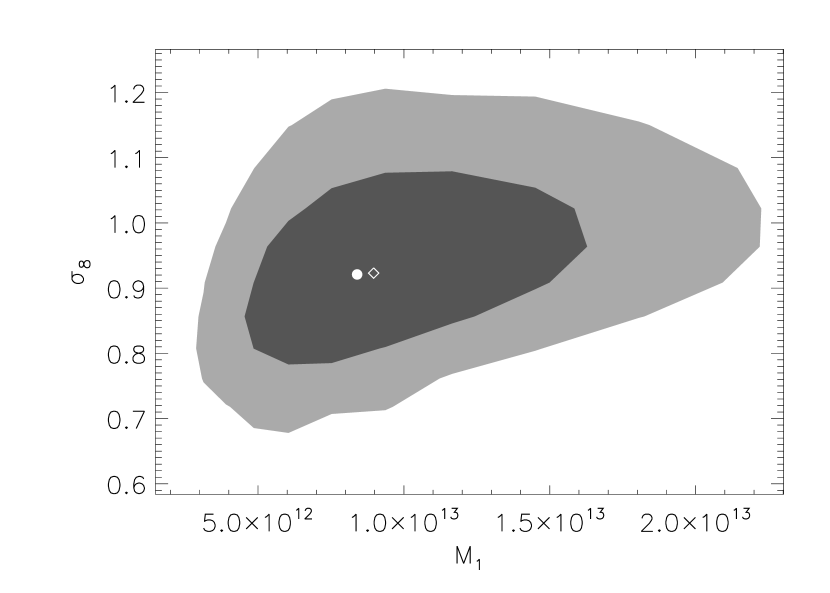
Figure 3.— Confidence regions ($68\%$ and $95\%$) in the $\sigma_{8}-M_{1}$ plane. The circle marks the median values of $M_{1}$ and $\sigma_{8}$ $(8.4\cdot 10^{12}M_{\odot},0.92)$, while the diamond marks the corresponding average values $(9\cdot 10^{12}M_{\odot},0.92)$. $\sigma_{8}$ and $M_{1}$ are the only two completely free parameters in our analysis.

A comparison between the observed number counts and the recovered maximum-likelihood model can be seen in Figure 2. We can see that our best fit model provides an excellent fit to the observed number counts. The corresponding $68\%$ and $95\%$ confidence regions in the $\sigma_{8}-M_{1}$ plane are seen in Figure 3. The median and average values for each of these two parameters are $(M_{1},\sigma_{8})=(8.4\cdot 10^{12}M_{\odot},0.92)$ and $(M_{1},\sigma_{8})=(9.0\cdot 10^{12}M_{\odot},0.92)$ respectively. The marginalized distribution for $\sigma_{8}$, shown in Figure 5, is roughly fit by a Gaussian distribution with $\sigma_{8}=0.92\pm 0.10$, and allows us to place an interesting lower limit on $\sigma_{8}$: $\sigma_{8}>0.76$ ($95\%$ CL) or $\sigma_{8}>0.68$ ($99\%$ CL). The $M_{1}$ distribution is roughly lognormal, though with some slight skewness. The corresponding $1-\sigma$ parameters are $\ln(M_{1}/10^{12}M_{\odot})=2.1\pm 0.4$, corresponding to $M_{1}=8.2^{+4.0}_{-2.7}\ \times 10^{12}M_{\odot}$.

While our remaining model parameters were all constrained with priors, it is nevertheless interesting to look at their a posteriori distributions. In particular, we find that there appears to be some tension between our prior on the slope $\beta$ of the $N_{obs}-N_{T}$ relation, and our prior on $\alpha$, the slope of the HOD. This is illustrated in Figure 4, where we show the posterior distribution in the $\alpha-\beta$ plane. The circle marks the median values of the marginalized distributions $(\beta,\alpha)=(1.15,0.84)$ whereas the square marks the central values of our priors, $\alpha=1.0$ and $\beta=1.18$. The average values of the parameters are very close to the median values. The degeneracy direction is roughly $\alpha\beta=constant$, as expected based on the fact that $N_{obs}\sim N_{T}^{\beta}\sim m^{\alpha\beta}$. While the width of our priors is large enough that we do not feel this discrepancy biases our results, it is clear from Figure 4 that either the slope of the $N_{obs}-N_{T}$ relation is shallower than seen in the simulations, or the slope of the HOD is markedly different from unity. Information from a new suite of simulations for currently ongoing work indicates that it is probably the former: our prior for $\beta$ seems to be on the high edge of what is possible.

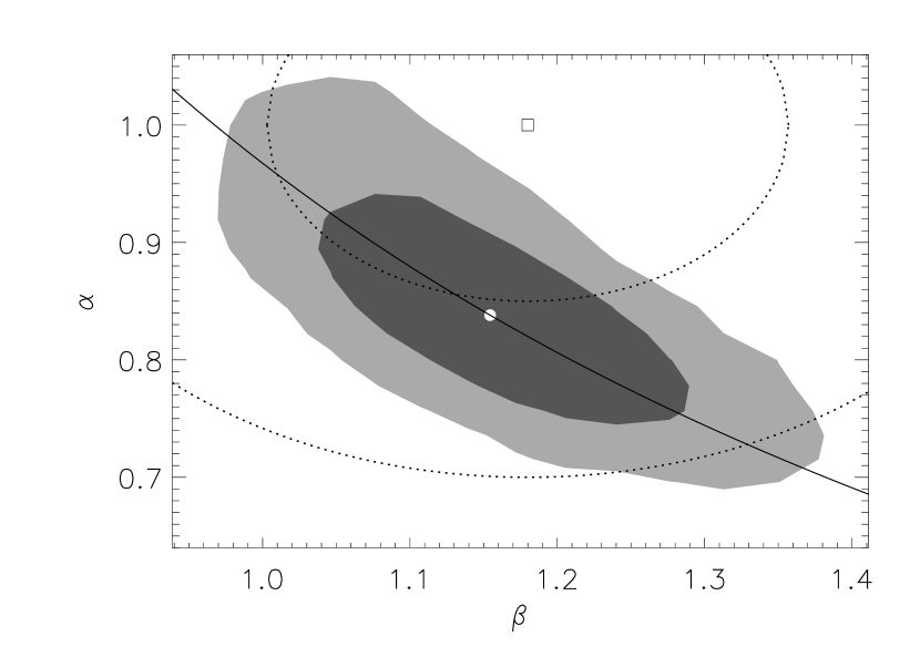
Figure 4.— The posterior distribution in the $\alpha-\beta$ plane. The filled contours represent the $68\%$ and $95\%$ confidence regions, which are centered on the square; also shown for reference are the corresponding regions in our prior distribution. The circle marks the median values of each of the parameters $(\beta,\alpha)=(1.15,0.84)$, which are almost identical to the average values. Note that the central value for our input priors (the square) lies outside the $95\%$ confidence region of the a posteriori distribution, suggesting that either our calibration is incorrect, or the slope of the HOD is substantially lower than unity. The solid line corresponds to the expected $\alpha\beta\approx\ constant$ degeneracy between the two parameters.

While it is impossible for us to fully determine whether the HOD prior or our simulation-calibrated prior is more incorrect without additional information, we can try to better understand how each of these two possibilities would affect our results. To do so, we have run two additional MCMCs, one with a tight, $5\%$ prior on $\alpha$ and no prior on $\beta$, and one with the converse priors. Due to the strong $\alpha\beta$ degeneracy, in either case we found that the maximum likelihood model resulted in an excellent fit to the data.

Our results are summarized in Figure 5. Briefly, we find that the tight $\beta$ prior favors a low $\alpha$ ($\alpha=0.76\pm 0.05$) and a very high $\sigma_{8}$ ($\sigma_{8}=1.05^{+0.13}_{-0.11}$), whereas the tight HOD prior $\alpha=1.0\pm 0.05$ favors a lower $\sigma_{8}$ value, $\sigma_{8}=0.92\pm 0.11$. The implausibly large value for $\sigma_{8}$ and the further lowering of $\alpha$ for the $\beta$ prior suggests that our central value for $\beta$ may be too high, which is consistent with more recent preliminary determinations of the maxBCG selection function in simulations of our ongoing work.

Figure 5.— The solid histogram shows the marginalized $\sigma_{8}$ distribution recovered from our MCMC. A Gaussian fit to the distribution results in $\sigma_{8}=0.92\pm 0.10$. From the above distribution we can also directly obtain a lower limit for $\sigma_{8}$, $\sigma_{8}>0.76$ at $95\%$ confidence, or $\sigma_{8}>0.68$ at $99\%$ confidence. Also shown are the marginalized distributions recovered when one places a tight, $5\%$ prior on the slope of the HOD (dotted line) and no prior on the selection function, and for the converse case (dashed line).

5. Discussion

5.1. Comparison With Other Work

We have performed a detailed statistical analysis of the observed cluster counts in the maxBCG cluster catalog of Koester et al. (2007b). We find $\sigma_{8}=0.92\pm 0.10$ (1-$\sigma$), and place an interesting lower limit $\sigma_{8}>0.75$ ($95\%$ CL) or $\sigma_{8}>0.66$ ($99\%$ CL). All of our results are marginalized over all major systematic effects, though they are also subject to additional cosmological priors $\Omega_{m}h^{2}=0.128\pm 0.01$ and $h=0.73\pm 0.05$. Finally, our analysis was restricted to flat cosmologies with massless neutrinos and scale-invariant primordial power spectra.

Our value for $\sigma_{8}$ is somewhat larger — but consistent with — the typical value obtained from cluster abundance studies using X-rays ($\sigma_{8}\approx 0.7$, see e.g. Borgani et al. 2001; Pierpaoli et al. 2001; Ikebe et al. 2002; Allen et al. 2003; Pierpaoli et al. 2003; Schuecker et al. 2003; Henry 2004, and references therein). $\sigma_{8}$ determinations from optical cluster samples are more rare, but here again we find our results to be in good agreement with previous work. For instance, both Berlind et al. (2006) and van den Bosch et al. (2006) suggest $\sigma_{8}\approx 0.8$, though no errors on this estimate are made. On the other hand, Rines et al. (2006) analyze a local cluster sample selected from the SDSS and report $\sigma_{8}=0.92^{+0.24}_{-0.19}$, similar to the result from Bahcall et al. (2003) and that of Bahcall & Bode (2003).

The work that is perhaps most directly comparable in spirit to ours is that of Gladders et al. (2006), who find $\sigma_{8}=0.67^{+0.18}_{-0.13}$ using a self-calibration technique to analyze cluster abundances as observed in the Red-Sequence Survey (RCS). As in our work, their value for $\sigma_{8}$ is marginalized over uncertainties in both the mass-richness relation and the hubble parameter $h$. This is particularly important as it is known that these are the parameters that are most highly degenerate with $\sigma_{8}$ (see e.g. Rozo et al. 2004), yet they are often held fixed in cluster abundance studies. Despite the fact that the central value for $\sigma_{8}$ in Gladders et al. (2006) is below our $99\%$ confidence lower limit $\sigma_{8}>0.68$, given the large error bars in both of our determinations it is clear that our results are, in fact, quite consistent with each other. Moreover, the likelihood function in Gladders et al. (2006) has a large tail that extends out to $\sigma_{8}\approx 1.2$, implying the overlap between the two analysis is even larger than what the $68\%$ confidence error bars might suggest.

What is clear at this time is that a precise determination of $\sigma_{8}$ still eludes us. This is unfortunate, as our large errors for $\sigma_{8}$ imply that almost any reasonable value that we could find would automatically be consistent with the $\Lambda CDM$ interpolated value found by Spergel et al. (2006), $\sigma_{8}=0.74^{+0.05}_{-0.06}$. It is evident that an improvement of at least a factor of two in the error bars is needed before $\sigma_{8}$ constraints from cluster abundances become a potential probe of the evolution of dark energy. Fortunately, such an improvement may be possible in the near future. For instance, we are now in the process of measuring weak lensing masses for clusters of fixed richness $N_{obs}$ using the method presented in Johnston et al. (2004) . In principle, such a measurement represents a direct measurement of the richness-mass relation, and hence can place direct constraints on the mass scale $M_{1}$ and the product $\alpha\beta$, the effective slope of the mass-richness relation.

An additional interesting result at this stage is the low value for $\alpha$, the slope of the HOD, that we recovered with our analysis. Whereas we find $\alpha=0.83\pm 0.06$, there is a significant body of evidence that points towards larger values of $\alpha$. From the observational side, Kochanek et al. (2003) obtain a slope $\alpha\approx 1$ or a little steeper on the basis of a 2MASS cluster sample obtained from a matched filter algorithm, though we note that a recent new analysis based on stacked X-ray emission from these clusters suggests a lower value $\alpha=0.87\pm 0.05$ (Dai et al. 2006). Likewise, Tinker et al. (2006) find a slope of unity based on the galaxy angular correlation function and the distribution of voids in the SDSS. Finally, Zehavi et al. (2005) find that the slope $\alpha$ is close to unity, but steadily increases with increasing luminosity. They also note, however, that this result is dependent on the detailed form of the HOD parameterization. In particular, an alternate parameterization from Kravtsov et al. (2004) with slope of unity on the high mass end is seen to be consistent with the data as well. From the theoretical side, Kravtsov et al. (2004) showed that the slope $\alpha$ characterizing the HOD of subhalos is very close to unity. Moreover, numerical simulations of galaxy formation suggest there is an excellent correspondence between dark matter subhalos and galaxies (Gao et al. 2004; Nagai & Kravtsov 2005; Weinberg et al. 2006). This is further evidenced by the fact that simple models used to assign luminosities to galaxies provide excellent matches to the luminosity dependent galaxy-galaxy and galaxy-mass correlations functions (Tasitsiomi et al. 2004; Mandelbaum et al. 2005; Conroy et al. 2006; Vale & Ostriker 2006), as well as the galaxy three-point function (Marin et al. 2007, in preparation).

There are, however, some lines of evidence for a lower value for $\alpha$. In particular, some numerical simulations suggest a value $\alpha\approx 0.8$ on the high mass end (Berlind et al. 2003). Also, Scoccimarro et al. (2001) cited a low value of the slope $\alpha=0.8$ on the basis of the galaxy three-point function, though we note they did not differentiate between central and satellite galaxies, which would tend to lower the recovered slope for the HOD. Abazajian et al. (2005) also found that the best fit value for $\alpha$ was $\alpha=0.83^{+0.22}_{-0.23}$ on the basis of a joint analysis of the galaxy angular correlation function and the CMB, though note the rather large error bars. Finally, analysis of the 2dFGRS cluster catalog of Yang et al. (2005b) also suggests that if $\sigma_{8}\approx 0.9$ then the number of galaxies in massive halos is low relative to standard models, consistent with a lower value for $\alpha$ (Yang et al. 2005a). Nevertheless, they emphasize their data is equally well fit by a low $\sigma_{8}$ model with a standard galaxy population, and in their most recent analysis they argue that a moderately low $\sigma_{8}$ (roughly $0.8\lesssim\sigma_{8}\lesssim 0.9$) is likely to be correct (van den Bosch et al. 2006).

Overall, the majority of the evidence available suggests that the slope of the HOD is typically closer to unity than what we have found. Of course, in general one expects that in detail, the slope of the HOD will depend on the particular criteria for galaxy selection in computing the HOD. At this point, about all we can say is that the maxBCG cluster sample provides some marginal evidence for $\alpha<1$, though this is only about a $2\sigma$ effect, and, moreover, the deviation from unity might be slightly overestimated if indeed the selection function in the simulations and in the real data are different.

5.2. Additional Sources of Systematics

An absolutely fundamental assumption about our statistical method is that the cluster selection function is an inherent property of the cluster-finding algorithm used. More specifically, we have assumed that given a halo of richness $N_{T}$, the cluster-finding algorithm has a probability $P(N_{obs}|N_{T})$ of detecting such a halo as a cluster of richness $N_{obs}$. If this probability is not a property of the cluster-finding algorithm (ie, if it is a strong function of cosmology), then our analysis needs to be generalized, and the cosmological dependence of the probability matrix needs to be calibrated. Consequently, the extent to which the above probability is robust to moderate changes in cosmology is an inherent systematic of our method, and clearly warrants further investigation. We emphasize, however, that this is true of any characterization of a cluster selection function obtained through the use of simulations. That is to say, it is not guaranteed a priori that two different yet realistic simulations will result in the same cluster selection function.

In addition to the above systematic, by far our most important uncertainties are due to possible selection effects not included within our model. For instance, we expect each of the components of our model — the completeness and purity functions and the signal matrix — to have some redshift and richness dependence. In this work, we have simply ignored this possibility, though we note that due to the small range of redshifts probed, we do not expect this systematic to be particularly significant. Moreover, we have explicitly demonstrated that ignoring such evolution in the simulations does not bias our results in any way (Rozo et al. 2007).

In addition to these selection function systematics, there are additional sources of error which we have not included. For instance, in this work we have ignored possible evolution in the HOD. Given the relatively narrow redshift range considered, and the fact that there appears to be little evolution in the way galaxies populate halos between redshifts $z=0$ and $z=0.8$ (Yan et al. 2003), we do not expect the no evolution assumption to be a limiting factor in our analysis.

A more theoretical systematic which we have not considered has to do with the current uncertainty in the predicted halo mass function. In particular, while the halo mass function appears to be universal with about a $\approx 20\%$ margin of error (Jenkins et al. 2001), additional work is required to test whether the halo mass function is indeed universal to higher accuracy — and if not, to characterize any intrinsic cosmological dependences. In this work, we have ignored these complications and have made no attempt to marginalize over the corresponding uncertainties (as is customary in the literature). We have, however, explicitly checked that changing the parameterization of the halo mass function from that of Jenkins et al. (2001) to that of Sheth & Tormen (2002) or that of Warren et al. (2005) changes the expectation values of our parameters by much less than our quoted $1\sigma$ uncertainty.

Yet another possible systematic of theoretical origin has to do with our assumptions about the HOD. In particular, if the HOD has any curvature over the mass range probed, then our model will necessarily result in biased parameter estimation. Since at this time we are only probing roughly one and a half decades in mass, we do not expect this to be a significant problem. Nevertheless, once the selection function for the maxBCG cluster-finding algorithm is better understood, it would be interesting to investigate to what extent the data can constrain deviations from linearity in the mean relation between halo mass and $N_{T}$.

5.3. Future Work and Improvements

Clearly, one of the most important problems to work on at this time is improving our understanding of the maxBCG selection function. Note that this work must involve investigating a large range of cosmological parameters so that any cosmology dependences inherent to the cluster-finding algorithm can be adequately calibrated. In addition, it is possible the simulations themselves need to be refined to produce more realistic skies so that differences in the cluster selection function between the simulations and the real sky are minimized.

Along this same line of reasoning, an important possibility that must be considered is to ask what the most useful richness definitions are, and its related question, what the best way of matching halos to clusters is. While we have done some preliminary work in this direction Rozo et al. (see 2007), we note that membership-based matching algorithms obviously depend on what we mean by a halo member. Thus, if the definition for $N_{T}$ changes, the matching of halos to clusters, i.e. the selection function, changes. Indeed, preliminary work suggests that uncertainties in the selection function of the cluster-finding algorithm are significantly reduced if only ridgeline galaxies are considered as halo members. Note that from a theoretical perspective, such a definition for $N_{T}$ would be perfectly fine, since galaxy formation models suggest that early type galaxies in clusters also obey a simple Poisson HOD (Zheng et al. 2005). Of course, the important thing is not the fact the HOD is Poisson, but that we have a theoretically well-motivated reason for choosing a particular form for the scatter between halo mass and richness.

Finally, it is evident that perhaps the single most important step at this time will be to include additional data that will soon be available for the maxBCG sample. Specifically, we are now in the process of computing ensemble-averaged X-ray, dynamical, and weak lensing masses for the SDSS maxBCG cluster sample. These new data sets will directly constrain the richness-mass relation of the clusters, and their inclusion will provide an entirely new tool that will further improve the cosmological constraints derived here.

In light of the above discussion, it is clear that there remains an enormous amount of work to be done to fully realize the potential of optical cluster catalogs. Nevertheless, we emphasize that, even in this first, roughest attempt to recover science from the SDSS maxBCG cluster sample, we have been able to derive robust cosmological constraints that are competitive with other approaches, squarely placing optical cluster science in the general toolkit of the precision cosmology effort.

Appendix A Definition of the Nuisance Parameters

Here we summarize the expressions that define the nuisance parameters in our model. For a discussion of where these expressions come from, we refer the reader to Rozo et al. (2007). The probability distribution $P(N_{obs}|N_{T})$ is characterized as follows: let $\mu_{ML}(N_{T})$ be the most likely value for $N_{obs}$ given $N_{T}$. $\mu_{ML}$ is parameterized as a power law

$$\mu_{ML}(N_{T})=20\exp(B_{0})(N_{T}/20)^{\beta},$$ (A1)

which defines $B_{0}$ and $\beta$. The mean value of $N_{obs}$ at fixed $N_{T}$ is found to be given by

$$\left\langle N_{obs}|N_{T}\right\rangle=20\exp(B_{0}+0.14)(N_{T}/20)^{(\beta-0.12)}$$ (A2)

and the variance is given by

$$\mbox{Var}(N_{obs}|N_{T})=\exp(-3B_{0}+B_{1})\mu(N_{T})$$ (A3)

which defines $B_{1}$. The confidence regions in the $B_{0}-B_{1}$ plane for each of the three simulations considered in Rozo et al. (2007) are seen in figure 6. The solid lines define a band over which the parameters $B_{0}$ and $B_{1}$ are allowed to vary.

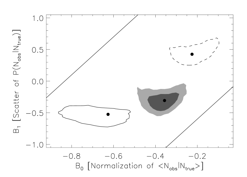
Figure 6.— $95\%$ confidence regions for the $B_{0}$ and $B_{1}$ in each of the three mock catalogs analyzed in Rozo et al. (2007). The dashed and solid contours are for Mocks A and B respectively. The shaded contours are $68\%$ and $95\%$ confidence regions in Mock C. The small filled circles mark the best-fit parameters from the mock catalogs, and were used to generate the Monte-Carlo realizations from which the confidence regions are derived. The solid lines mark the band over which the parameters $B_{0}$ and $B_{1}$ are allowed to vary.

The completeness function is observed to be richness independent, and is thus parameterized in terms of a single parameter $c$ such that $c(N_{T})=c$. The purity function is characterized with two parameters $p_{0}$ and $p_{1}$ such that

$$p(N_{obs})=\exp(-x(N_{obs})^{2})$$ (A4)

where

$$x(N_{obs})=p_{0}+p_{1}\left(\frac{\ln(15)}{\ln(N_{obs})}-1\right).$$ (A5)

Finally, the photometric redshift distribution $\rho(z_{c}|z_{h})$ where $z_{c}$ is the observed photometric redshift of a cluster and $z_{h}$ is the true spectroscopic redshift of the parent halo is taken to be of the form

$$\rho(z_{c}|z_{h})=\frac{1}{z_{h}}\rho_{b}(b|z_{h})$$ (A6)

where $b=z_{c}/z_{h}$ is the photometric redshift bias. $\rho_{b}$ is found to be Gaussian, and the nuisance parameters $\left\langle b_{z}\right\rangle$ and $\sigma_{z}$ correspond to the mean and standard deviations of said Gaussian.

References

- Abazajian et al. (2005) Abazajian, K., Zheng, Z., Zehavi, I., Weinberg, D. H., Frieman, J. A., Berlind, A. A., Blanton, M. R., Bahcall, N. A., Brinkmann, J., Schneider, D. P., & Tegmark, M. 2005, ApJ, 625, 613
- Allen et al. (2003) Allen, S. W., Schmidt, R. W., Fabian, A. C., & Ebeling, H. 2003, MNRAS, 342, 287
- Bahcall & Bode (2003) Bahcall, N. A. & Bode, P. 2003, ApJ, 588, L1
- Bahcall et al. (2003) Bahcall, N. A., Dong, F., Bode, P., Kim, R., Annis, J., McKay, T. A., Hansen, S., Schroeder, J., Gunn, J., Ostriker, J. P., Postman, M., Nichol, R. C., Miller, C., Goto, T., Brinkmann, J., Knapp, G. R., Lamb, D. O., Schneider, D. P., Vogeley, M. S., & York, D. G. 2003, ApJ, 585, 182
- Berlind et al. (2006) Berlind, A. A., Kazin, E., Blanton, M. R., Pueblas, S., Scoccimarro, R., & Hogg, D. W. 2006, ArXiv Astrophysics e-prints
- Berlind et al. (2003) Berlind, A. A., Weinberg, D. H., Benson, A. J., Baugh, C. M., Cole, S., Davé, R., Frenk, C. S., Jenkins, A., Katz, N., & Lacey, C. G. 2003, ApJ, 593, 1
- Bond et al. (1991) Bond, J. R., Cole, S., Efstathiou, G., & Kaiser, N. 1991, ApJ, 379, 440
- Borgani et al. (2001) Borgani, S., Rosati, P., Tozzi, P., Stanford, S. A., Eisenhardt, P. R., Lidman, C., Holden, B., Della Ceca, R., Norman, C., & Squires, G. 2001, ApJ, 561, 13
- Conroy et al. (2006) Conroy, C., Wechsler, R. H., & Kravtsov, A. V. 2006, ApJ, 647, 201
- Dai et al. (2006) Dai, X., Kochanek, C. S., & Morgan, N. D. 2006, ArXiv Astrophysics e-prints
- Dunkley et al. (2005) Dunkley, J., Bucher, M., Ferreira, P. G., Moodley, K., & Skordis, C. 2005, MNRAS, 356, 925
- Eisenstein & Hu (1999) Eisenstein, D. J. & Hu, W. 1999, ApJ, 511, 5
- Eke et al. (1996) Eke, V. R., Cole, S., & Frenk, C. S. 1996, MNRAS, 282, 263
- Evrard et al. (2002) Evrard, A. E., MacFarland, T. J., Couchman, H. M. P., Colberg, J. M., Yoshida, N., White, S. D. M., Jenkins, A., Frenk, C. S., Pearce, F. R., Peacock, J. A., & Thomas, P. A. 2002, ApJ, 573, 7
- Gao et al. (2004) Gao, L., De Lucia, G., White, S. D. M., & Jenkins, A. 2004, MNRAS, 352, L1
- Gladders et al. (2006) Gladders, M. D., Yee, H. K. C., Majumdar, S., Barrientos, L. F., Hoekstra, H., Hall, P. B., & Infante, L. 2006, Cosmological Constraints from the Red-Sequence Cluster Survey
- Hansen et al. (2005) Hansen, S. M., McKay, T. A., Wechsler, R. H., Annis, J., Sheldon, E. S., & Kimball, A. 2005, ApJ, 633, 122
- Henry (2004) Henry, J. P. 2004, ApJ, 609, 603
- Holder (2006) Holder, G. 2006, astro-ph/0602251
- Holder et al. (2001) Holder, G., Haiman, Z., & Mohr, J. J. 2001, ApJ, 560, L111
- Hu & Cohn (2006) Hu, W. & Cohn, J. D. 2006, Phys. Rev. D, 73, 067301
- Ikebe et al. (2002) Ikebe, Y., Reiprich, T. H., Böhringer, H., Tanaka, Y., & Kitayama, T. 2002, A&A, 383, 773
- Jenkins et al. (2001) Jenkins, A., Frenk, C. S., White, S. D. M., Colberg, J. M., Cole, S., Evrard, A. E., Couchman, H. M. P., & Yoshida, N. 2001, MNRAS, 321, 372
- Johnston et al. (2004) Johnston, D., Sheldon, E., Koester, B., Wechsler, R., McKay, T., Frieman, J., Annis, J., Evrard, A., Zehavi, I., Scranton, R., Nichol, R., Connolly, A., Budavari, T., Tasitsiomi, A., & SDSS. 2004, American Astronomical Society Meeting Abstracts, 205, 147.06
- Kochanek et al. (2003) Kochanek, C. S., White, M., Huchra, J., Macri, L., Jarrett, T. H., Schneider, S. E., & Mader, J. 2003, ApJ, 585, 161
- Koester et al. (2007a) Koester, B. P. et al. 2007a, ApJ, in press, astro-ph/0701268
- Koester et al. (2007b) —. 2007b, ApJ, in press, astro-ph/0701265
- Kravtsov et al. (2004) Kravtsov, A. V., Berlind, A. A., Wechsler, R. H., Klypin, A. A., Gottlöber, S., Allgood, B., & Primack, J. R. 2004, ApJ, 609, 35
- Mandelbaum et al. (2005) Mandelbaum, R., Tasitsiomi, A., Seljak, U., Kravtsov, A. V., & Wechsler, R. H. 2005, MNRAS, 362, 1451
- Molnar et al. (2004) Molnar, S. M., Haiman, Z., Birkinshaw, M., & Mushotzky, R. F. 2004, ApJ, 601, 22
- Nagai & Kravtsov (2005) Nagai, D. & Kravtsov, A. V. 2005, ApJ, 618, 557
- Navarro et al. (1997) Navarro, J. F., Frenk, C. S., & White, S. D. M. 1997, ApJ, 490, 493 (NFW)
- Pierpaoli et al. (2003) Pierpaoli, E., Borgani, S., Scott, D., & White, M. 2003, MNRAS, 342, 163
- Pierpaoli et al. (2001) Pierpaoli, E., Scott, D., & White, M. 2001, MNRAS, 325, 77
- Press & Schechter (1974) Press, W. H. & Schechter, P. 1974, ApJ, 187, 425
- Rines et al. (2006) Rines, K., Diaferio, A., & Natarajan, P. 2006, The Virial Mass Function of Nearby SDSS Galaxy Clusters
- Rozo et al. (2004) Rozo, E., Dodelson, S., & Frieman, J. A. 2004, Phys. Rev. D, 70, 083008
- Rozo et al. (2007) Rozo, E., Wechsler, R. H., Koester, B. P., Evrard, A. E., & McKay, T. A. 2007, ApJ, submitted
- Schuecker et al. (2003) Schuecker, P., Böhringer, H., Collins, C. A., & Guzzo, L. 2003, A&A, 398, 867
- Scoccimarro et al. (2001) Scoccimarro, R., Sheth, R. K., Hui, L., & Jain, B. 2001, ApJ, 546, 20
- Sheth & Tormen (2002) Sheth, R. K. & Tormen, G. 2002, MNRAS, 329, 61
- Spergel et al. (2006) Spergel, D. N. et al. 2006, ArXiv Astrophysics e-prints
- Tasitsiomi et al. (2004) Tasitsiomi, A., Kravtsov, A. V., Wechsler, R. H., & Primack, J. R. 2004, ApJ, 614, 533
- Tinker et al. (2006) Tinker, J. L., Weinberg, D. H., & Warren, M. S. 2006, Cosmic Voids and Galaxy Bias in the Halo Occupation Framework
- Vale & Ostriker (2006) Vale, A. & Ostriker, J. P. 2006, Mon. Not. Roy. Astron. Soc., 371, 1173
- van den Bosch et al. (2005) van den Bosch, F. C., Weinmann, S. M., Yang, X., Mo, H. J., Li, C., & Jing, Y. P. 2005, MNRAS, 361, 1203
- van den Bosch et al. (2006) van den Bosch, F. C., Yang, X., Mo, H. J., Weinmann, S. M., Maccio, A., More, S., Cacciato, M., Skibba, R., & Xi, K. 2006, ArXiv Astrophysics e-prints
- Warren et al. (2005) Warren, M. S., Abazajian, K., Holz, D. E., & Teodoro, L. 2005, ArXiv Astrophysics e-prints
- Weinberg et al. (2006) Weinberg, D. H., Colombi, S., Dave, R., & Katz, N. 2006, Baryon Dynamics, Dark Matter Substructure, and Galaxies
- Yan et al. (2003) Yan, R., Madgwick, D. S., & White, M. 2003, ApJ, 598, 848
- Yang et al. (2005a) Yang, X., Mo, H. J., Jing, Y. P., & van den Bosch, F. C. 2005a, MNRAS, 358, 217
- Yang et al. (2005b) Yang, X., Mo, H. J., van den Bosch, F. C., & Jing, Y. P. 2005b, MNRAS, 356, 1293
- Zehavi et al. (2005) Zehavi, I., Zheng, Z., Weinberg, D. H., Frieman, J. A., Berlind, A. A., Blanton, M. R., Scoccimarro, R., Sheth, R. K., Strauss, M. A., Kayo, I., Suto, Y., Fukugita, M., Nakamura, O., Bahcall, N. A., Brinkmann, J., Gunn, J. E., Hennessy, G. S., Ivezić, Ž., Knapp, G. R., Loveday, J., Meiksin, A., Schlegel, D. J., Schneider, D. P., Szapudi, I., Tegmark, M., Vogeley, M. S., & York, D. G. 2005, ApJ, 630, 1
- Zheng et al. (2005) Zheng, Z., Berlind, A. A., Weinberg, D. H., Benson, A. J., Baugh, C. M., Cole, S., Davé, R., Frenk, C. S., Katz, N., & Lacey, C. G. 2005, ApJ, 633, 791