Three-dimensional Magnetohydrodynamic Simulations of
Cold Fronts in Magnetically Turbulent ICM
Abstract
Steep gradients of temperature and density, called cold fronts, are observed by Chandra in a leading edge of subclusters moving through the intracluster medium (ICM). The presence of cold fronts indicates that thermal conduction across the front is suppressed by magnetic fields. We carried out three-dimensional magnetohydrodynamic (MHD) simulations including anisotropic thermal conduction of a subcluster moving through a magnetically turbulent ICM. We found that turbulent magnetic fields are stretched and amplified by shear flows along the interface between the subcluster and the ambient ICM. Since magnetic fields reduce the efficiency of thermal conduction across the front, the cold front survives at least . We also found that a moving subcluster works as an amplifier of magnetic fields. Numerical results indicate that stretched turbulent magnetic fields accumulate behind the subcluster and are further amplified by vortex motions. The moving subcluster creates a long tail of ordered magnetic fields, in which the magnetic field strength attains .
1 Introduction
X-ray observations of clusters of galaxies by ASCA revealed complex temperature distributions in the intracluster medium (ICM), in which hot and cool plasma coexists (e.g, Perseus Cluster, Arnaud et al. 1994; Furusho 2001). Sharp discontinuities of density and temperature in ICM, called cold fronts, were found by high spatial resolution observations by Chandra (Markevitch et al., 2000; Vikhlinin et al., 2001b). Cold fronts manifest the coexistence of hot and cool plasma in clusters of galaxies. They provide a key to understand thermal properties of the ICM.
Cold fronts in merging clusters such as A2142, A3667, and 1E0657-56 result from merging. When a subcluster is moving in the ICM, a sharp boundary is formed between the subcluster and the ambient hot ICM in the forehead of the subcluster because the cold plasma confined by the subcluster is subjected to the ram pressure. The cold fronts are not shock fronts because the Chandra images of the X-ray surface brightness show that the temperature decreases on the denser side. A3667 has a clear, large-scale (), arc-shaped cold front which shows a steep gradient of the X-ray surface brightness and temperature. The temperature decreases toward the denser part from to within . This thickness of the front is 2-3 times smaller than the Coulomb mean free path (Vikhlinin et al., 2001b).
A question which needs to be answered is how the temperature gradient is
created and sustained in the ICM which typically has high Spitzer
conductivity,
(Spitzer, 1962).
Thermal conduction rapidly smooths such a steep gradient (e.g.,
Takahara & Ikeuchi 1977). The time required for heat to diffuse by conduction
across a length in the ICM is roughly given by
,
where is the density.
Ettori & Fabian (2000) and Markevitch et al. (2003) estimated that the effective thermal
conduction is at least an order of magnitude lower than the Spitzer
value.
This suggests that the thermal conduction across the front is suppressed
by magnetic fields parallel to the front (Vikhlinin et al., 2001b). Vikhlinin et al. (2001a)
suggested that ordered magnetic fields are formed in front of the
subcluster because small-scale turbulent magnetic fields are compressed
and stretched along the front ahead of the subcluster by its motion.
Typical clusters of galaxies possess magnetic fields of
(e.g., Kronberg 1994; Carilli & Taylor 2002).
Johnston-Hollitt (2004) reported that fields, tangled on
scale pervade the central region of A3667. When
magnetic fields exist, the characteristic scale of the heat exchange
across the field lines is reduced significantly compared with
non-magnetized ICM to the Larmor radius,
.
Intracluster magnetic fields play a crucial role for thermal conduction
even if the magnetic pressure is lower than the gas pressure.
A number of authors reported that cold fronts were reproduced in numerical simulations as a result of a merging process (e.g., Bialek et al. 2002; Nagai & Kravtsov 2003; Heinz et al. 2003; Acreman et al. 2003; Takizawa 2005). In these simulations, however, magnetic fields and thermal conduction were not included. To study the evolution of intracluster magnetic fields, Roettiger et al. (1999) performed MHD simulations of merging clusters and Dolag et al. (2002) performed cosmological MHD simulations. However, they ignored the thermal conduction. Asai et al. (2004) performed two-dimensional (2D) MHD simulations of a subcluster moving through uniform magnetic fields by including anisotropic thermal conduction. They showed that ordered magnetic fields wrap the subcluster and suppress the thermal conduction across the front. This work was extended to three-dimension by Asai et al. (2005).
Some authors pointed out that the effective conductivity in turbulent magnetic fields is only several times lower than the Spitzer value (Narayan & Medvedev, 2001). Dolag et al. (2004) carried out cosmological hydrodynamic simulations including the thermal conduction with the isotropic effective conductivity, and showed that temperature gradients are smoothed compared to the case without thermal conduction. However, a moving subcluster may stretch the turbulent magnetic fields and such fields may reduce the conductivity.
Lyutikov (2006) studied the magnetic draping mechanism by which a strongly magnetized, thin boundary layer with a tangential magnetic field is created in the boundary between a moving cloud and the ambient plasma. He theoretically predicted that for supersonic cloud motion, magnetic field strength inside the layer reaches near equipartition values with thermal pressure.
Asai et al. (2004) carried out a simulation starting from a disordered magnetic field and showed that cold fronts can be sustained because magnetic fields are stretched along the front and wrap the subcluster. However, their simulation was limited to 2D and their initial magnetic field still had a large coherent length. Thus magnetic fields can easily suppress the thermal conduction across the front.
In this paper, we present results of three-dimensional (3D) MHD simulations of a subcluster moving through turbulent magnetic fields to show that even when magnetic fields are turbulent, cold fronts can be sustained. The paper is organized as follows. In §2, we describe the initial condition and model parameters. Simulation results are presented in §3: we show the effects of magnetic fields on cold fronts and amplification of magnetic fields behind the subcluster. Finally, we discuss and summarize our results in §4.
2 Simulation Model
We simulated the time evolution of a cluster plasma in a frame comoving with the subcluster. The basic equations are as follows:
| (1) |
| (2) |
| (3) |
| (4) |
where , , , , and are the density, velocity, pressure, magnetic fields, and gravitational potential, respectively. We use the specific heat ratio . The subscript denotes the components parallel to the magnetic field lines. We assume that heat is conducted only along the magnetic field lines. We solved equations (1)-(4) in a Cartesian coordinate system by using a solver based on a modified Lax-Wendroff method (Rubin & Burstein, 1967) with artificial viscosity (Richtmyer & Morton, 1967) implemented to the Coordinated Astronomical Numerical Software (CANS). We did not include the physical viscosity. Artificial viscosity is included only in regions close to the discontinuities to suppress numerical oscillations. It does not affect the dynamics in smooth regions. The thermal conduction term in the energy equation is solved by the implicit red and black successive over-relaxation method (see Yokoyama & Shibata, 2001, for detail). The radiative cooling term is not included. The units of length, velocity, density, pressure, temperature, and time in our simulations are , , , , , and , respectively.
We carried out simulations for 6 models. Table 1 shows the model parameters. When magnetic fields exist, heat conducts only parallel to the magnetic field lines. Model MT1 and MT2 are models with turbulent magnetic fields. We define Fourier components of magnetic vector potential, , where is a wave number. The amplitudes are taken to be random by using random numbers, and we adopt . This vector potential in -space is transformed to vector potential in physical space via a 3D fast Fourier transform (FFT). We computed a tangled divergence-free initial magnetic field via . On the other hand, models MU1 and MU2 are models with uniform magnetic fields parallel to the -direction and perpendicular to the motion of the subcluster.
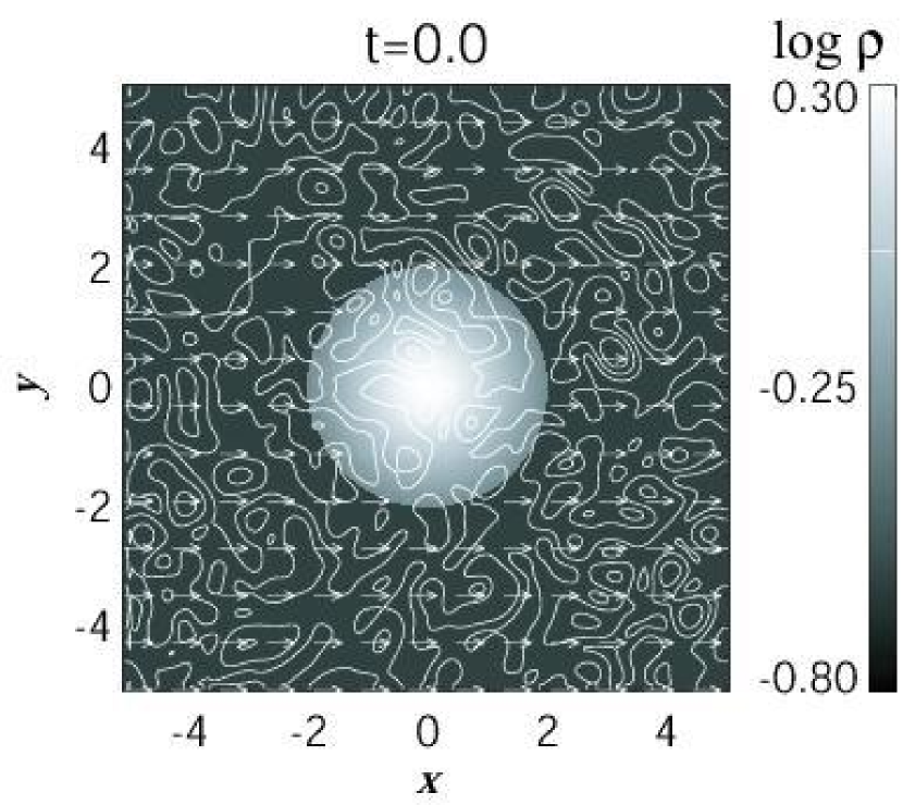
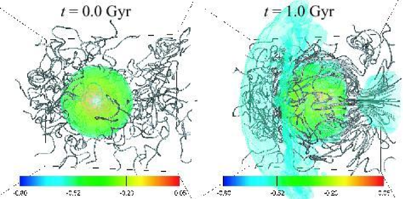
Figure 1 shows the initial density distribution for model MT1 at plane. Solid curves and arrows show the contours of magnetic field strength and velocity vectors, respectively. We assume that a spherical isothermal low-temperature () plasma is confined by the gravitational potential of the subcluster. The subcluster has a -model density distribution,
| (5) |
where we adopted , the core radius , and the maximum density . The subcluster is embedded in the low density (), hot () ambient plasma. We assume that the subcluster is initially in hydrostatic equilibrium and has a jump of density and temperature with respect to the ambient plasma. We also assume that the ambient plasma has a uniform speed , where is the ambient sound speed. Note that magnetic fields exist even inside the subcluster in all models with magnetic fields. The box size of our simulations is . We used grid points for typical models. The numerical resolution is .
An important parameter is plasma defined as the ratio of the gas pressure to the magnetic pressure (see Table 1). The initial mean field strength is for model MT1 and for model MT2. Correspondingly, initial plasma for these models is and , respectively. For models with uniform fields, the strength is for models MU1 and for model MU2. The initial plasma for these models is and , respectively. Model MT3 is the same as model MT1 except that thermal conduction is ignored and the box size of the -direction is times larger than that of model MT1. We also carried out a simulation for a model without magnetic fields (model H), including isotropic thermal conduction.
For turbulent field models (MT1, MT2, and MT3), the left boundary at is taken to be the fixed boundary, except for the magnetic fields. The magnetic fields at the left boundary are extracted from the initial distribution of magnetic fields as follows,
| (6) |
where is the initial magnetic field, and are mesh numbers in the and directions, is the total number of grid points in the -direction, is the initial velocity of the subcluster, and is the time. For other models, the left boundary is taken to be a fixed boundary. In all models, boundaries other than the left boundary are free boundaries where waves can be transmitted.
3 Results
3.1 Time Evolution of a Subcluster and Magnetic Fields
Figure 2 shows time evolution of density distribution and magnetic fields for model MT1. The left panel shows the initial state and the right panel shows the distribution at . Solid curves show the magnetic field lines. Since the subcluster plasma moves with sound speed, a bow shock appears ahead of the subcluster. Magnetic field lines are stretched along the subcluster surface at due to the ambient gas motion. Thus, the motion of the subcluster creates ordered magnetic fields along the interface between the subcluster and ambient ICM. The magnetic fields accumulate behind the subcluster.
3.2 Effect of Magnetic Fields on Thermal Conduction
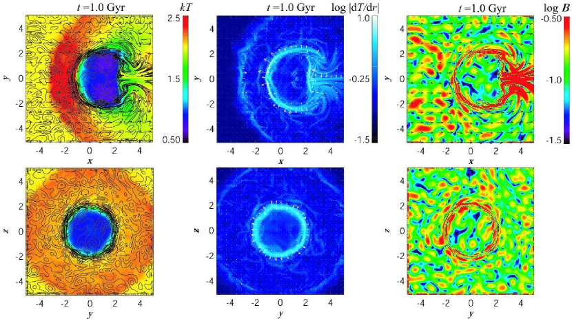
Figure 3 shows snap shots of distributions of temperature (left panels), temperature gradients (middle panels), and magnetic field strength (right panels) at . The upper panels show the slices at plane and the bottom panels show the slices at plane for model MT1, respectively. Solid curves in the left panels are the contours of magnetic field strength. Arrows in the left (and right) panels show the velocity vectors, and those in the middle panels are the gradients of temperature.
The temperature distributions (left panels) show that steep temperature gradients are maintained at because the thermal conduction across the front is suppressed by stretched magnetic field lines wrapping the subcluster. The middle panels show that steep temperature gradients around the subcluster surface are sustained. The cold front is located at in plane (upper panels). We can also identify the bow shock at in plane. The steepest temperature gradient is seen in the vicinity of in the upper middle panel. The distributions in plane (bottom panels) clearly show that the subcluster is almost entirely covered with magnetic fields.
In the left and right panels of Figure 3, we can see that magnetic fields are stretched and compressed around the subcluster as we already mentioned. A shear flow along the boundary between the subcluster and the ambient plasma stretches magnetic fields. Moreover, magnetic field strength is amplified behind the subcluster (see §3.3 for details). The field amplification is more prominent in the tail of the subcluster than in the forehead. The amplification of magnetic fields ahead of the cold fronts is due to the compression of magnetic fields by the ambient plasma flow hitting the subcluster. The ambient plasma flowing along the subcluster surface converges to the -axis behind the subcluster. Therefore, magnetic fields frozen to the plasma accumulates behind the subcluster.
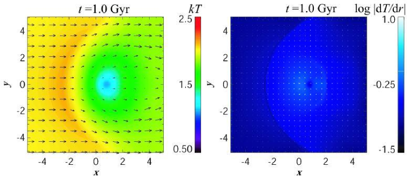
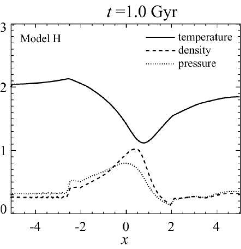
In order to demonstrate the effects of magnetic fields on thermal conduction, we present results of hydrodynamic model (model H) in Figure 4. The left and right panels show the distributions of temperature and temperature gradients. Compared with the results shown in Figure 3, temperature gradients are smeared out because isotropic thermal conduction from the ambient hot plasma rapidly heats up the dense cool plasma confined in the subcluster.
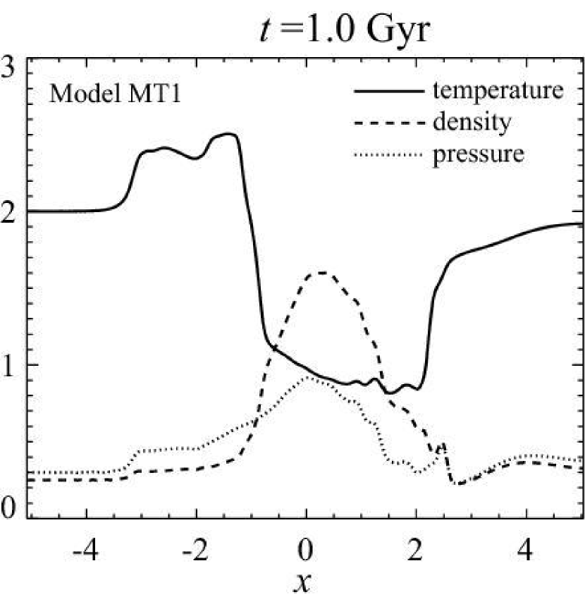
In Figure 5, we show the distributions of quantities at along the -axis (). The left and right panels show the distributions of temperature (solid curve), density (dashed curve), and pressure (dotted curve) for models MT1 and H. The temperature distribution in the left panel shows that a steep gradient exists at , while pressure distribution is smooth. This feature is consistent with the observed features of cold fronts (e.g., Markevitch et al. 2000). On the other hand, when magnetic fields do not exist (right panel), the subcluster plasma is subjected to the isotropic thermal conduction. After , the subcluster evaporates because of the conduction from the ambient hot plasma. The peak density in the subcluster becomes lower than that in the initial state.
3.3 Amplification of Magnetic Fields
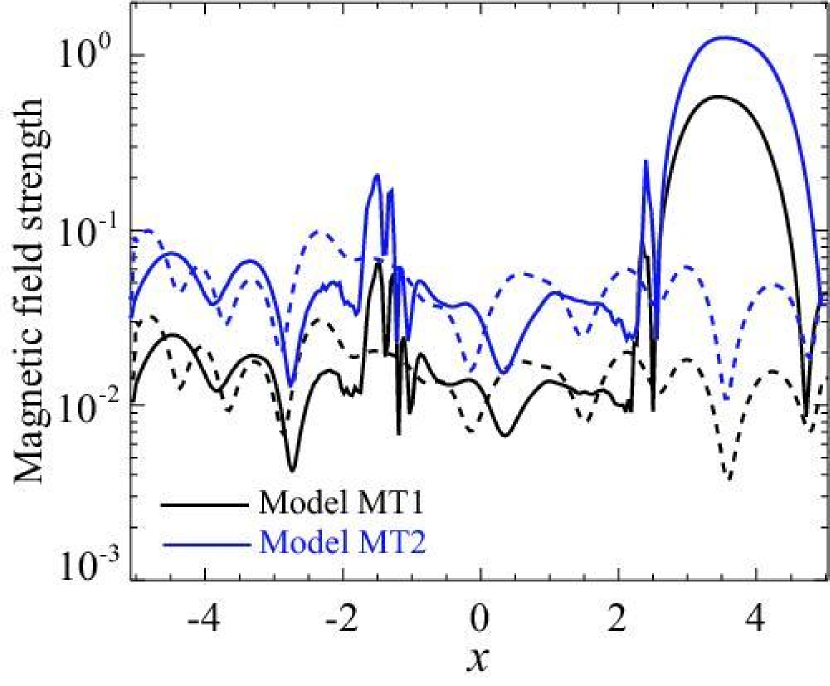
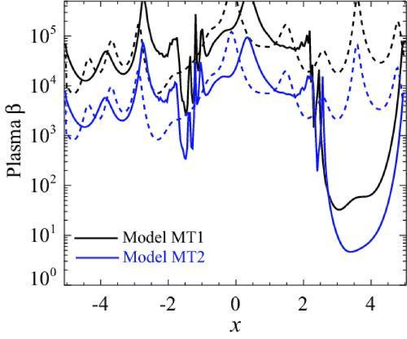
Simulation results revealed other interesting features. We found that a moving subcluster works as an amplifier of magnetic fields. The left panel of Figure 6 shows the distributions of magnetic field strength for the turbulent field models (models MT1 and MT2). The right panel shows the distributions of plasma . We plot these distributions along for model MT1 (black curves) and for model MT2 (blue curves), respectively. Solid curves in both panels are distributions at and dashed curves show those at the initial state, respectively. When turbulent fields exist, field strength is amplified in front of the subcluster and behind it. The amplification of the field strength is most prominent behind the subcluster. The field strength in both models increases about 30 times with respect to the averaged initial value. The right panel shows that plasma in both models decreases. In model MT2, plasma decreases below in the tail of the subcluster.
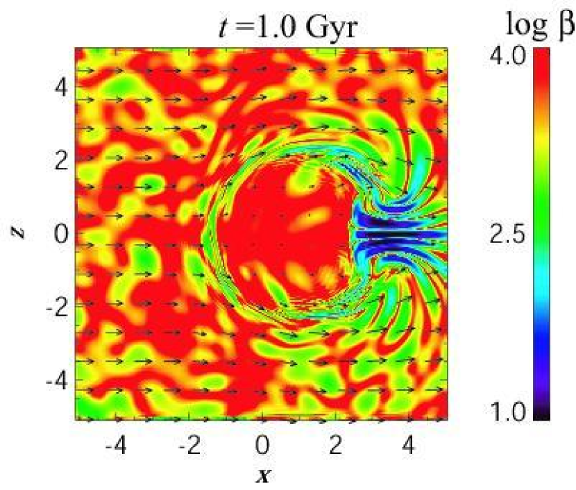
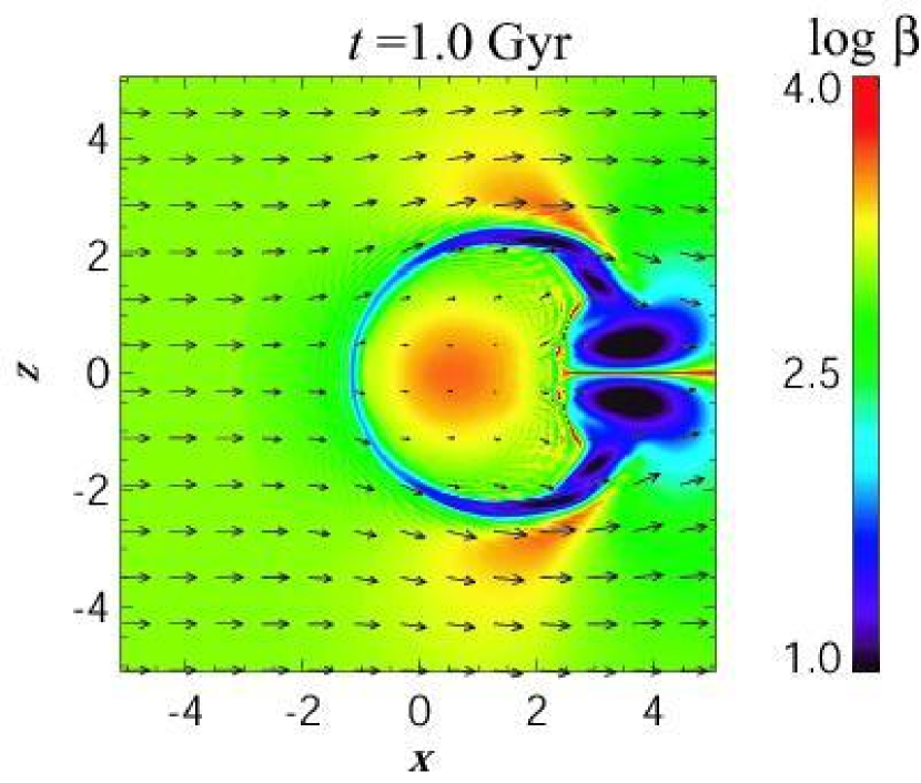
Let us compare the results for the turbulent field models with those of uniform field models. Figure 7 shows the distribution of plasma at along plane for model MT2 (left) and that for model MU2 (right). Note that the initial direction of magnetic fields for model MU2 is parallel to the -axis. In both panels, plasma decreases remarkably behind the subcluster. The plasma in this region is lower than . The region of lower plasma is larger for model MU2 than that for model MT2 because the initial magnetic fields are uniform in model MU2, thus the ambient plasma flow creates the ordered fields easily behind the subcluster. An important finding is that plasma decreases to behind the subcluster even if the initial magnetic fields are turbulent.
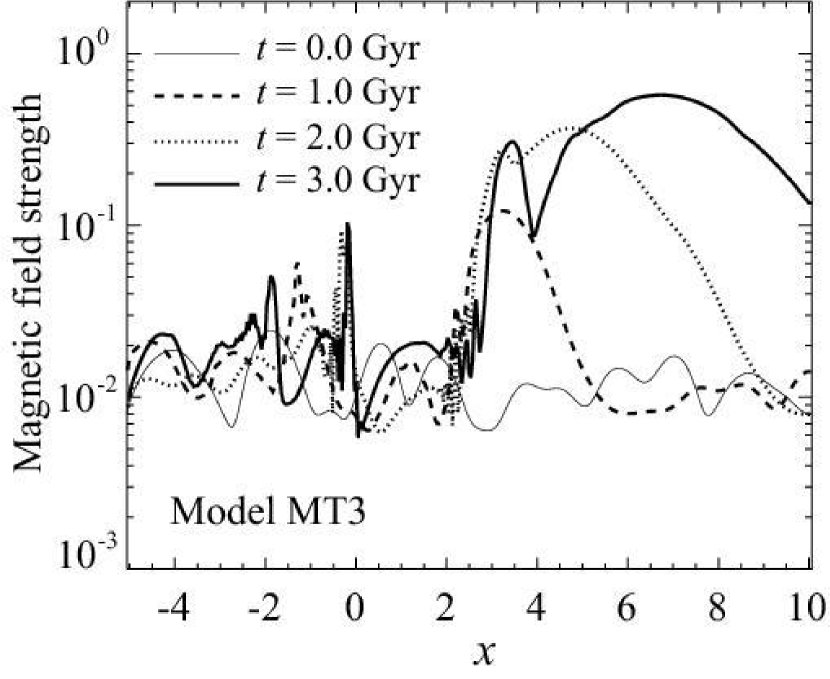
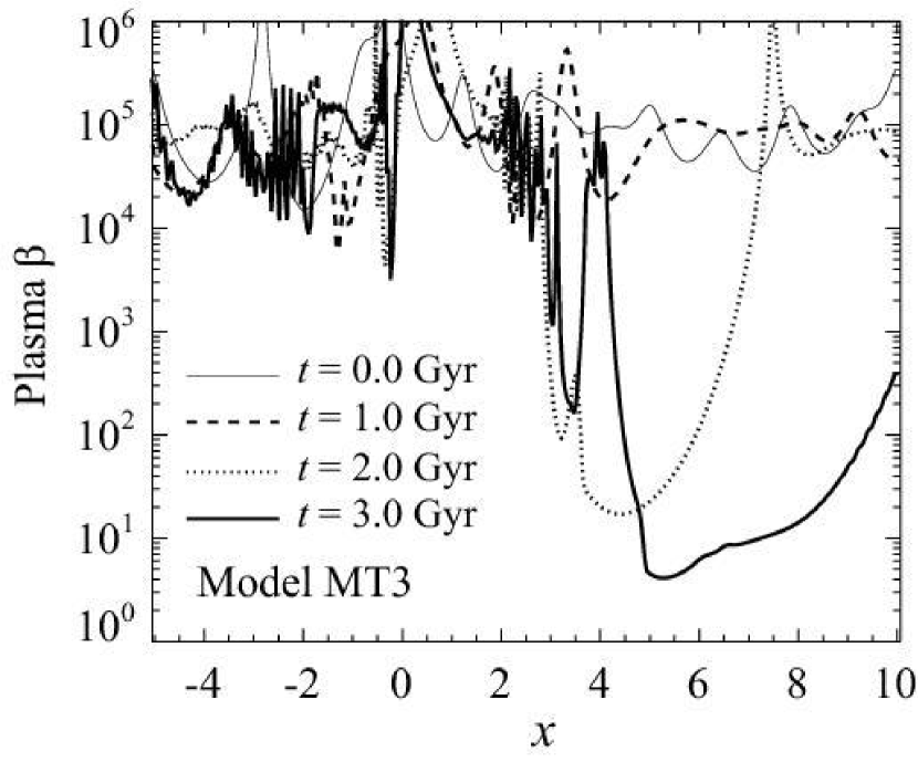
In model MT3, we used larger simulation box and carried out a simulation until in order to follow the growth of magnetic fields behind the subcluster. The size of simulation box for model MT3 is times larger in the -direction than that for other models. Figure 8 shows the distributions of magnetic field strength (left) and plasma (right) along the -direction () for model MT3. Curves in both panels show the distribution at (thin solid curve), (dashed curve), (dotted curve), and (thick solid curve). Magnetic fields are amplified with time behind the subcluster. They are accumulated around at . The flow motion stretches magnetic fields along the -direction. At , magnetic field strength peaks around . This strength is about 80 times higher than the initial value. In the right panel, the minimum plasma appears at . In this region, the plasma is smaller than 10.
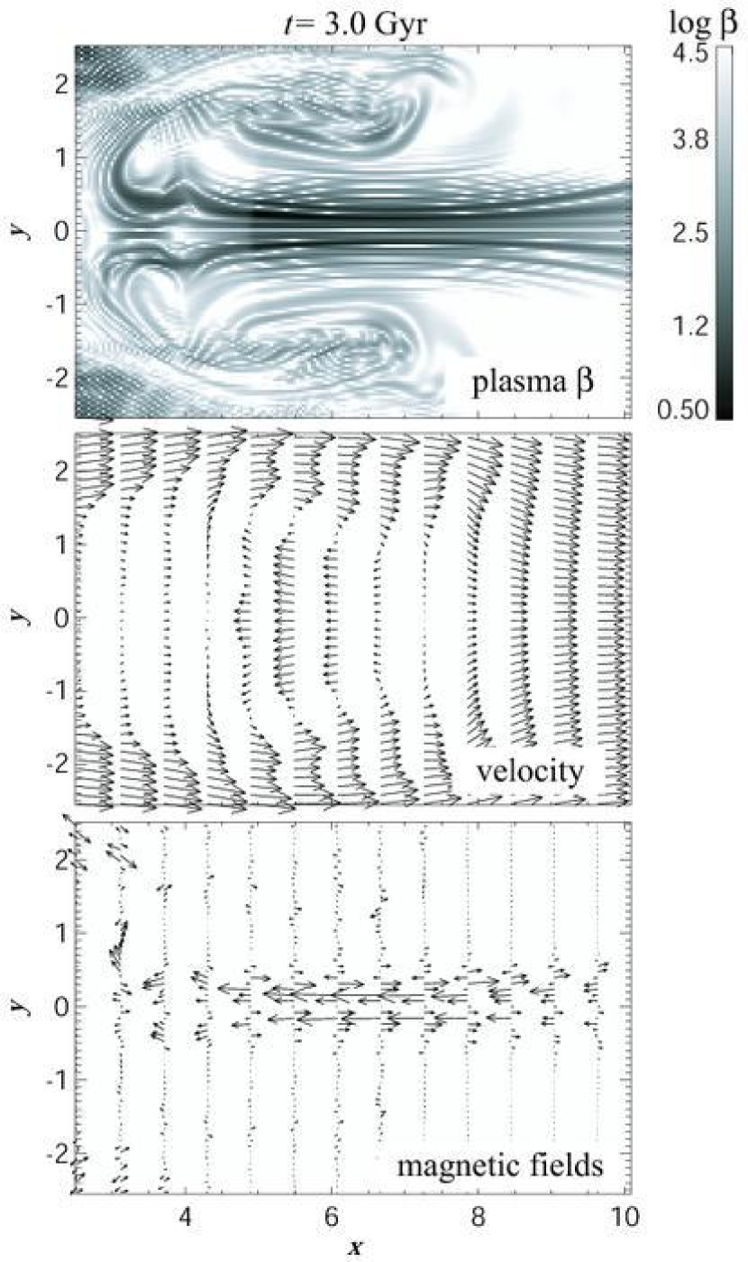
Figure 9 shows the distributions of plasma , velocity vectors, and magnetic field vectors in plane at for model MT3. The region behind the subcluster, , , is shown. The front of the subcluster is not shown here (it is located at ). The top panel shows that along the -axis (). We found that the ambient gas passing through the subcluster generates vortices behind the subcluster. They create back flows along the -axis (see middle panel). The back flow is similar to that reported by Heinz et al. (2003). Magnetic fields dragged by the gas flow are thus stretched along the -axis behind the subcluster. The -component of magnetic fields is particularly strengthened in the vicinity of the -axis (see bottom panels).
4 Discussion and Summary
We carried out 3D MHD simulations of a subcluster moving through a magnetically turbulent ICM in order to study the effects of magnetic fields on thermal conduction. We assumed that a dense, cold subcluster with a sharp discontinuity in density and temperature is moving with sound speed.
In this paper, we studied whether a cold front can be sustained in a magnetically turbulent ICM. In §3.1 and §3.2, we demonstrated that a cold front is maintained for over because magnetic fields stretched along the front suppress the thermal conduction across the front even if magnetic fields are initially turbulent. On the other hand, when magnetic fields do not exist, steep temperature gradients cannot be maintained because the cold subcluster is heated up due to the isotropic thermal conduction. Therefore, we conclude that cold fronts in merging clusters can exist because magnetic fields coupled with the motion of the subcluster suppress the thermal conduction.
In §3.3, we showed that magnetic fields are amplified significantly behind the subcluster because the ambient flow converges to the tail of the subcluster. The flow accumulates magnetic fields to this tail region. Furthermore, the vortex motions behind the subcluster accumulates and stretches the magnetic fields. The enhanced fields are maintained for a long time behind the subcluster. Thus, the motion of a subcluster forms a long tail of ordered magnetic fields. It may be worth noting that the magnetic filaments created behind the subcluster are similar to the magnetic filaments in the solar atmospheres, in which the magnetic fields are accumulated in boundaries of the convective cell. Plasma decreases to . If such a long tail of magnetic fields interacts with other moving subclumps, magnetic fields will be further amplified. Consequently, small-scale weak magnetic fields in the ICM can be amplified and create large-scale magnetic fields whose energy is comparable to the thermal energy. This mechanism may also apply to the amplification of small-scale primordial magnetic fields once dark matter clumps are formed.
References
- Acreman et al. (2003) Acreman D. M., Stevens I. R., Ponman T. J., & Sakelliou I., 2003, MNRAS, 341,1333
- Arnaud et al. (1994) Arnaud, K. A., et al. 1994, ApJ, 436, L67
- Asai et al. (2004) Asai, N., Fukuda, N., & Matsumoto, R. 2004, ApJ, 606, L105
- Asai et al. (2005) Asai, N., Fukuda, N., & Matsumoto, R. 2005, Adv. Sp. Res., 36, 636
- Bialek et al. (2002) Bialek, J. J., Evrard, A. E., & Mohr, J.J., 2002, ApJ, 578, L9
- Carilli & Taylor (2002) Carilli, C. L., & Taylor, G. B. 2002, ARA&A, 40, 319
- Dolag et al. (2002) Dolag, K., Bartelmann, M., & Lesch, H., 2002, A&A, 387, 383
- Dolag et al. (2004) Dolag, K., Jubelgas, M., Springel, V., Borgani, S., & Rasia, E., 2004, ApJ, 606, L97
- Ettori & Fabian (2000) Ettori, S., & Fabian, A. C. 2000, MNRAS, 317, L57
- Furusho (2001) Furusho, T., Yamasaki, N. Y., Ohashi, T., Shibata, R., & Ezawa, H. 2001, ApJ, 561, L165
- Heinz et al. (2003) Heinz, S., Churazov, E., Forman, W., Jones, C., & Briel, U. G. 2003, MNRAS, 346, 13
- Johnston-Hollitt (2004) Johnston-Hollitt, M. 2004, in The Riddle of Cooling Flows in Galaxies and Clusters of Galaxies, ed. T. H. Reiprich, J. C. Kempner, & N. Soker, http://www.astro.virginia.edu/coolflow/
- Kronberg (1994) Kronberg, P. P. 1994, Rep. Prog. Phys., 57, 325
- Lyutikov (2006) Lyutikov, M. 2006, MNRAS, 373, 73
- Markevitch et al. (2000) Markevitch, M., et al. 2000, ApJ, 541, 542
- Markevitch et al. (2003) Markevitch, M., et al. 2003, ApJ, 589, L19
- Nagai & Kravtsov (2003) Nagai, D., & Kravtsov, A. V., 2003, ApJ, 587, 514
- Narayan & Medvedev (2001) Narayan, R., & Medvedev, M. V. 2001, ApJ, 562, L129
- Richtmyer & Morton (1967) Richtmyer, R., O., & Morton, K., W. 1967, Differential Methods for Initial Value Probrem (2d ed., New York: Wiley)
- Roettiger et al. (1999) Roettiger, K., Stone, J. M., & Burns, J. O., 1999, ApJ, 518, 594
- Rubin & Burstein (1967) Rubin, E., & Burstein, S., Z. 1967, J. Comput. Phys., 2, 178
- Spitzer (1962) Spitzer, L. 1962, Physics of Fully Ionized Gases (2d ed.; New York: Intersciense)
- Takahara & Ikeuchi (1977) Takahara, F., & Ikeuchi, S. 1977, Prog. Theor. Phys., 58, 1728
- Takizawa (2005) Takizawa, M., 2005, ApJ, 629, 791
- Vikhlinin et al. (2001a) Vikhlinin, A., Markevitch, M., & Murray, S. S. 2001a, ApJ, 549, L47
- Vikhlinin et al. (2001b) Vikhlinin, A., Markevitch, M., & Murray, S. S. 2001b, ApJ, 551, 160
- Yokoyama & Shibata (2001) Yokoyama, T., & Shibata, K. 2001, ApJ, 549, 1160
| Model | aa is the thermal conductivity, and the subscript denotes the component parallel to magnetic field lines. | magnetic field | bbfootnotemark: | ccfootnotemark: | box size [] | number of grids |
|---|---|---|---|---|---|---|
| MT1 | turbulent | |||||
| MT2 | turbulent | |||||
| MU1 | uniform | |||||
| MU2 | uniform | |||||
| MT3 | 0 | turbulent | ||||
| H | — |
 .
.