On estimating redshift and luminosity distributions in photometric redshift surveys

Abstract

The luminosity functions of galaxies and quasars provide invaluable information about galaxy and quasar formation. Estimating the luminosity function from magnitude limited samples is relatively straightforward, provided that the distances to the objects in the sample are known accurately; techniques for doing this have been available for about thirty years. However, distances are usually known accurately for only a small subset of the sample. This is true of the objects in the Sloan Digital Sky Survey, and will be increasingly true of the next generation of deep multi-color photometric surveys. Estimating the luminosity function when distances are only known approximately (e.g., photometric redshifts are available, but spectroscopic redshifts are not) is more difficult. I describe two algorithms which can handle this complication: one is a generalization of the $V_{\rm max}$ algorithm, and the other is a maximum likelihood approach. Because these methods account for uncertainties in the distance estimate, they impact a broader range of studies. For example, they are useful for studying the abundances of galaxies which are sufficiently nearby that the contribution of peculiar velocity to the spectroscopic redshift is not negligible, so only a noisy estimate of the true distance is available. In this respect, peculiar velocities and photometric redshift errors have similar effects. The methods developed here are also useful for estimating the stellar luminosity function in samples where accurate parallax distances are not available.

1 Introduction

Estimates of the distribution of distances to galaxies, and of the galaxy luminosity function and its evolution, provide useful constraints on models of galaxy formation. Current (e.g. the SDSS, York et al. 2000, Combo-17, Wolf et al. 2003, MUSYC, Marchesini et al. 2007) and planned surveys (e.g., DES, LSST) go considerably deeper in multicolor photometry than in spectroscopy, or are entirely photometric. For such surveys, reasonably accurate photometric redshift estimates (e.g. Hyper-$z$, Bolzonella et al. 2000, and ANN$z$, Collister & Lahav 2003) can or will be made. In the case of Luminous Red Galaxies (e.g. Eisenstein et al. 2001), the photometric redshifts may actually be quite accurate (e.g. Padmanabhan et al. 2004; Weinstein et al. 2004; Collister et al. 2006). The number of objects with photometric redshifts typically exceeds the number for which spectroscopic redshifts are available by more than an order of magnitude. This is also true of new quasar detection algorithms. Whereas the SDSS will obtain spectra of about one hundred thousand quasars, the Non-parametric Bayesian Classification algorithm of Richards et al. (2004) has identified one million quasars using SDSS photometry. Large photometric samples of galaxies and quasars offer the potential of studying cosmological evolution at a fraction of the cost of a full spectroscopic survey.

Bigger is not better only for studying the evolution of the galaxy and quasar populations. In the case of galaxies, the larger number of LRGs with photometric redshifts, allowed new science: the detection of the integrated Sachs-Wolfe effect (Fosalba et al. 2003; Scranton et al. 2003; Padmanabhan et al. 2005; Cabre et al. 2006) required the larger photometric LRG catalog. In the case of quasars also, larger sample sizes allow one to address new science questions. For example, the SDSS spectroscopic sample is barely large enough to measure the gravitational lensing magnification bias signal with high statistical significance: the larger photometric sample made the measurement possible (Scranton et al. 2005).

With photometric redshift surveys becoming the norm, it is timely to devise methods for estimating the distribution of comoving distances and the evolution of the luminosity function in such samples. Broadly speaking, techniques for estimating the luminosity function from a magnitude limited catalog fall into two classes: one is based on the nonparametric $V_{max}$ method outlined by Schmidt (1968); the other is a maximum likelihood analysis which can provide parametric or nonparametric estimates of the luminosity function (Sandage, Tammann & Yahil 1979; Efstathiou, Ellis & Peterson 1988; Springel & White 1998). Both methods assume that the distances are known precisely and accurately. The main goal of the present work is to generalize both types of methods to handle photometric redshifts. For reasons described below, the analysis which follows is best-suited to studying objects where evolution and $k$-correction uncertainties are small. In practice, this means they are best suited to catalogs which contain objects of one spectral type. Removing this constraint is the subject of ongoing work.

Section 2 discusses a deconvolution algorithm for estimating $dN/dz$ and the luminosity function from photometric redshift samples. The estimator of the luminosity function is a generalization of the $V_{\rm max}$ method (Schmidt 1968), and the method uses the deconvolution algorithm described by Lucy (1974). Section 3 discusses a maximum likelihood approach. Some applications are discussed in Section 4 and a final section summarizes.

2 The $V_{\rm max}$ method

I first outline why the problems of estimating $dN/dz$ and $\phi(L)$ are both best thought of as deconvolution problems. I then show that Lucy’s deconvolution algorithm provides an efficient way of performing the deconvolution.

2.1 The redshift distribution: $dN/dz$

Let $dN/dz$ denote the number of objects which lie at redshift $z$ (since peculiar velocities are unlikely to be larger than a few thousand km/s, they do not make a significant change to the redshift if $z>0.01$). Let $p(z_{e}|z)$ denote the probability of estimating the redshift as $z_{e}$ when the true value is $z$. Then the distribution of estimated redshifts is

$${dN_{e}(z_{e})\over dz_{e}}=\int dz\,{dN(z)\over dz}\,p(z_{e}|z).$$ (1)

To get an idea of what this implies, suppose that $p(z_{e}|z)$ is sharply peaked around the true value $z$. Then define $\Delta z\equiv z_{e}-z$ and expand $dN/dz$ in a Taylor series around its value at $z_{e}$. This yields an expansion in $\Delta z$. If the estimated redshift is unbiased in the mean, then $\langle\Delta z\rangle=0$ and the leading order contribution is of the form

$${dN_{e}(z_{e})\over dz_{e}}\approx{dN(z_{e})\over dz_{e}}+{\langle\Delta z^{2}\rangle\over 2}\,{\partial^{2}[dN(z)/dz]\over\partial z^{2}}\Biggl{|}_{z_{e}}$$ (2)

Typically, $dN/dz$ is well approximated by a constant times $z^{2}\,\exp[-(z/z_{m})^{\alpha}]$, with $\alpha\approx 3/2$ and $z_{m}$ set by the luminosity function and the limiting magnitude of the catalog (i.e., $dN/dz\propto z^{2}$ at $z\ll z_{m}$, and it drops rapidly for $z\gg z_{m}$). In this case,

$${dN_{e}(z_{e})\over dz_{e}}\approx{dN(z_{e})\over dz_{e}}\left[1+{\langle\Delta z^{2}\rangle\over z_{e}^{2}}\,C(z_{e})\right],$$ (3)

where

$$C(z_{e})=1-{3\alpha\over 2}\left({z_{e}\over z_{*}}\right)^{\alpha}-{\alpha^{2}\over 2}\left({z_{e}\over z_{*}}\right)^{\alpha}+{\alpha^{2}\over 2}\left({z_{e}\over z_{*}}\right)^{2\alpha}.$$ (4)

The term in square brackets shows how the estimated distribution $dN_{e}$ differs from the true one $dN$. In particular, it shows that an accurate estimate of $dN$ can be obtained by summing over all objects that have estimated redshift $z_{e}$, weighting each by the inverse of the term in square brackets in the expression above.

The general problem is to infer the shape of the intrinsic distribution $dN/dz$ given the measured distribution $dN_{e}/dz_{e}$, even if $p(z_{e}|z)$ is not sharply peaked. If $p(z_{e}|z)$ is known, and $dN_{e}/dz_{e}$ is measured, then this is an integral equation of the first kind, which can be solved to obtain the intrinsic $dN/dz$. This is possible even if $p(z_{e}|z)$ is fairly broad. Padmanabhan et al. (2004) describe a method to do this, but, for reasons made explicit in Lucy (1974), their method is not ideal. Before we describe our method, the following section shows that estimating the intrinsic luminosity function from photometric redshift data is a similar deconvolution problem.

2.2 The luminosity distribution: $\phi(L)$

Let $\phi(M|z)$ denote the number density of galaxies with absolute magnitudes $M\propto-2.5\log_{10}L$, where $L=\ell\,4\pi D_{L}^{2}(z)$ is the luminosity, $\ell$ is the apparent brightness, and $D_{L}(z)$ is the luminosity distance at $z$. Assume for the moment that there is no evolution (extending the analysis to include evolution is the subject of work in progress). Then $\phi(M|z)$ is independent of $z$.

Simply adding up the total number of galaxies in a magnitude limited catalog which have luminosity $L$ and dividing by the total volume of the survey is not a good estimator of $\phi(L)$ itself. This is because the more luminous objects will be visible to larger distances. Let $V_{\rm max}(M)$ denote the largest comoving volume out to which an object of absolute magnitude $M$ can be seen. If the catalog is limited at both ends, then there is a minimum volume below which the object would have been too bright to be included in the catalog: call this $V_{min}(M)$. The number of galaxies with absolute magnitude $M$ in a catalog magnitude limited at both ends is

$$N(M)=\phi(M)\,\Bigl{[}V_{\rm max}(M)-V_{\rm min}(M)\Bigr{]}.$$ (5)

Therefore, if we sum over all the galaxies in a magnitude limited catalog, and we weight each object by the inverse of $V_{\rm max}(M)-V_{\rm min}(M)$, then we will actually have estimated the luminosity function. This is the basis of the $1/V_{\rm max}$ method (Schmidt 1968).

If the estimate $z_{e}$ of the true redshift $z$ comes with a large uncertainty, this translates into an uncertainty in the luminosity (this assumes that the error in redshift determination does not affect the observed apparent magnitude). The total number of objects with estimated absolute magnitudes $M_{e}$ is

$$N_{e}(M_{e}) = \int_{m_{\rm min}}^{m_{\rm max}}{\rm d}m\,\int{\rm d}D_{\rm L}\,n(m,D_{\rm L})\,p(m-M_{e}|D_{\rm L},m)$$ (6)

$$= \int{\rm d}D_{\rm L}{{\rm d}V_{\rm com}\over{\rm d}D_{\rm L}}\int_{M_{\rm min}(D_{\rm L})}^{M_{\rm max}(D_{\rm L})}{\rm d}M\,\phi(M)\,$$

$$\qquad\qquad\qquad\qquad\times\quad p(M-M_{e}|D_{\rm L},M)$$

$$= \int{\rm d}M\,\phi(M)\int_{D_{\rm L}(M_{\rm min})}^{D_{\rm L}(M_{\rm max})}{\rm d}D_{\rm L}{{\rm d}V_{\rm com}(D_{\rm L})\over{\rm d}D_{\rm L}}$$

$$\qquad\qquad\times\quad p(M-M_{e}|D_{\rm L},M),$$

where we have used the fact that $5\log_{10}D_{e}=m-M_{e}=5\log_{10}D_{\rm L}+M-M_{e}$, so $p(D_{e}|D_{\rm L},m)\,{\rm d}D_{e}=p(M-M_{e}|D_{\rm L},m)\,{\rm d}M_{e}$. Note that if there is no error in the distance, then $p(M-M_{e})$ is a delta function centered on $M$, and this expression reduces to equation (5).

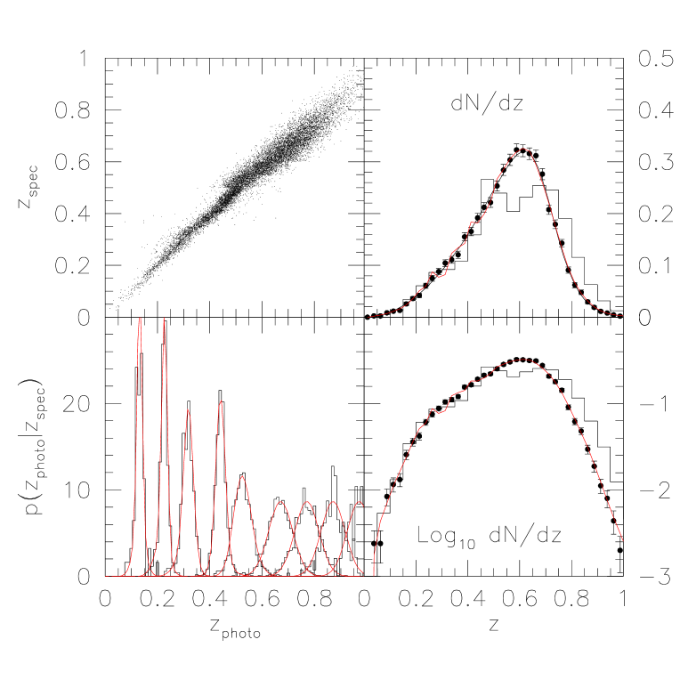
Figure 1: Example of the difference between the intrinsic redshift distribution (filled circles with error bars in panels on right) and the photometric redshift distribution (histograms in panels on right). Panels on the left compare the intrinsic and estimated redshifts. Jagged lines in panels on right show how successive iterations converge rapidly to the intrinsic distribution: the histogram was used as the starting guess.

If ${\cal V}(V_{\rm max},V_{\rm min},M)$ denotes result of performing the integral over $D_{\rm L}$ in the final expression above, then

$$N_{e}(M_{e})=\int{\rm d}M\,\phi(M)\,{\cal V}(V_{\rm max},V_{\rm min},M).$$ (7)

Since $V_{\rm max}$ and $V_{\rm min}$ are known functions of $M$, ${\cal V}$ itself is really just a complicated function of $M$. To get some feel for its form, suppose that the error in determining the redshift does not depend on apparent magnitude, and, in addition, the error distribution is a function of the ratio $D_{e}/D_{\rm L}$ only. Then $p(M-M_{e}|D_{\rm L},M)$ does not depend explicitly on $D_{\rm L}$ itself, so it can be taken out of the integral over $D_{\rm L}$. In this case,

$${\cal V}=\Bigl{[}V_{\rm max}(M)-V_{\rm min}(M)\Bigr{]}\,p(M_{e}|M),$$ (8)

Now, $\phi(M)$ times the term in square brackets is the intrinsic $N(M)$ distribution (equation 5), so equation (7) becomes

$$N_{e}(M_{e})=\int{\rm d}M\,N(M)\,p(M_{e}|M).$$ (9)

In this case, the observed distribution of $M_{e}$ is the convolution, not just of the luminosity function $\phi$ with the error distribution $p$, but of the product of $\phi$ and $(V_{\rm max}-V_{\rm min})$ with $p$. The inclusion of this second term accounts for the fact that more objects are likely to scatter down from large $z$ to small than the other way around, simply because there is a greater volume at larger $z$. The form of the expression above shows clearly that one generically expects distance errors to scatter objects from the peak of the $N(M)$ distribution to the tails. Unless it is corrected for, this will lead one to overestimate the number density of low and high luminosity objects relative to the mean.

When the distances are known accurately, one can simply use $\phi=N/V$ as a non-parametric estimate of the luminosity function. However, the expression above shows that the relation between $N_{e}(M_{e})$ and $\phi$ is more complicated than when the distance is not known precisely: determining $\phi$ requires solution of an integral equation. In this respect, the problem is similar to that of determining $dN/dz$ when $dN_{e}/dz_{e}$ and $p(z_{e}|z)$ are known. Once again, in the case of small errors, one can expand the integrand in a power series and then perform the integral to determine the correction factor $C(M_{e})$ that is required if one wishes to weight galaxies by $1/[(1+C)V]$ and so estimate $\phi$ from the number of observed $M_{e}$. But the general case is more complicated.

Before moving on to the solution, note that the assumption that $p(M-M_{e}|D_{\rm L},M)$ does not depend explicitly on $D_{\rm L}$ itself, is not crucial. I have mainly made the assumption here so that the form of the argument is clear. If it does depend on $D_{\rm L}$, then the weighting factor in the integrand is a more complicated function of $M$ than simply $N(M)\,p(M_{e}|M)$.

2.3 Non-parametric deconvolution and the $V_{\rm max}$ method

Since $N_{e}(M_{e})$, $p(M_{e}|M)$ and ${\rm d}V_{\rm com}/{\rm d}z$ are all known, the relation to be solved for $\phi(M)$ is an integral equation of the first kind. Standard arguments show that it can be written as a matrix equation which can then be solved for $\phi(M)$. The problem with this approach is how one accounts for the fact that the measured $N_{e}(M_{e})$ distribution may be noisy. In particular, since $N_{e}(M_{e})$ is likely to be smoother than $N(M)$, if $N_{e}$ contains sharp features, then the recovered $N$ will contain sharper features. If sharp features are expected to be unrealistic, and the measurement is noisy (this will always be true in the tails), then an exact inversion of the integral equation is clearly undesirable. An iterative algorithm which avoids this problem was proposed by Lucy (1974); it converges rapidly and is simple to code ($\sim 20$ lines of code), so it is the method of choice.

Figure 1 shows how well this method works on mock data. Mock galaxies were distributed in redshift as indicated by the filled circles in the right-hand panels of Figure 1. Estimated redshifts were assigned as shown in the bottom left panel (the particular choice of $p(z_{e}|z)$ will be discussed shortly). Top left panel compares the estimated and true redshifts. The histograms in the panels on the right show the distribution of estimated redshifts. Note how different they are from the true distribution: although $dN/dz$ has a single well-defined peak, $dN_{e}/dz_{e}$ is almost bimodal. Our choice of $p(z_{e}|z)$ was chosen to produce just this effect: it mimics the effect on some photometric redshift estimators as, e.g., the 4000Å break passes from one filter to another. The problem is to use the estimated histogram and the known shape of $p(z_{e}|z)$ to infer that the true intrinsic distribution traces the locus defined by the filled circles. The histogram was used as the starting guess for the deconvolution algorithm, after which the algorithm converged rapidly to the filled circles (four iterations are shown; they overlap one another closely). Figure 2 provides a more detailed comparison of how well the recovered distribution resembles the true one, and how different the photo-$z$ distribution, which was used as the starting guess, is from the true distribution.

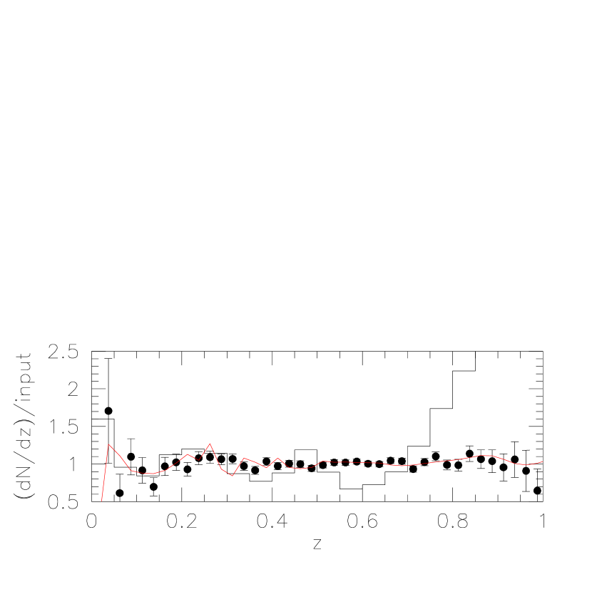
Figure 2: Comparison of true intrinsic redshift distribution and that recovered by the algorithm described in the text. Symbols with error bars show one realization of the intrinsic distribution (the difference from unity is ‘shot-noise’ due to the finite size of the sample). Histogram shows the associated photo-$z$ distribution, and jagged curve shows the recovered distribution after four iterations: the histogram was used as the starting guess.

Figure 3 shows results for the luminosity function. The panel on the left shows the intrinsic $N(M)$ (solid circles) and estimated $N_{e}(M)$ (open circles) distributions in a mock catalog generated assuming the same flat cosmological model as before, but with the intrinsic distribution of luminosities and the apparent magnitude limits chosen to be those of the galaxies in the SDSS survey (Blanton et al. 2003). The estimated redshifts were assumed to follow $p(D_{e}|D)dD_{e}=(dx/x)(\gamma x)^{\gamma}\exp(-\gamma x)/\Gamma(\gamma)$, where $x=D_{e}/D$ and $\gamma=5$. This distribution has $\langle x\rangle=1$, and $\sigma^{2}_{x}=1/\gamma$. With $\gamma=5$, this error distribution is substantially worse than typical photometric redshift errors. Notice how $N(M_{e})$ is broader than the true distribution: it has noticably more objects in the tails, and hence fewer near the peak. This is the generic effect we mentioned earlier.

The open circles in the panel on the right show the result of converting from $N_{e}(M)$ to $\phi(M)$ using Schmidt’s method with no correction for the photometric redshift error distribution. This estimate has more luminous galaxies, and a steeper faint-end slope, than the true distribution shown by the solid circles. For photo-$z$ error distributions which are approximately symmetric, this sort of discrepancy is generic.

The solid lines in the panel on the left show successive iterations of the deconvolution algorithm, starting from the open circles. Convergence to the correct distribution is clearly seen. The solid line in the panel on the left shows the result of applying Schmidt’s method to the estimate of $N(M)$ returned by the final iteration shown. It is an excellent approximation to the intrinsic distribution.

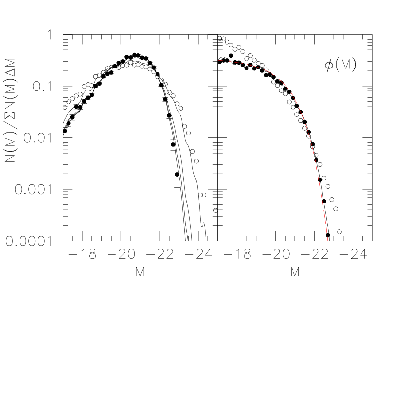
Figure 3: Reconstruction of the intrinsic $N(M)$ distribution (filled circles) from the distribution of estimated redshifts when distance uncertainties are large (open circles). Error bars on the filled circles assume Poisson statistics. Different curves show how successive iterations of the deconvolution algorithm approximate the intrinsic distribution increasingly well: the open circles were used as the starting guess, and curves show results after iterations 1, 8, 15, and 22. Panel on the left shows the observed distribution, and panel on the right shows the associated estimate of the luminosity function. Dashed curve shows the input luminosity function. The generic effect of photo-$z$ errors, which the deconvolution algorithm rectifies (compare solid line with filled circles), is to enhance the large luminosity tail, and steepen the faint end slope (compare open with filled circles).

To illustrate that the generic effect of distance errors is to scatter objects from the peak of $N(M_{e})$ into the tails, thus increasing the expected number of high luminosity objects and increasing the slope at small luminosities, Figure 5 shows a similar calculation, but now when the true intrinsic luminosity function is a Gaussian in absolute magnitude. The precise parameter values were chosen to match those of early-type galaxies in the SDSS, and, once again, I have assumed photo-$z$ error distributions (Gaussian with 1 mag rms) that are significantly broader than most photo-$z$ algorithms return. Notice again how the algorithm rapidly converges from the observed counts (open circles) to the true ones (filled circles).

3 The maximum-likelihood method

In magnitude limited samples, an unbiased estimate of the luminosity function is obtained by maximizing the (log of the) likelihood function

$${\cal L}({{\mbox{\boldmath$a$}}}) = \prod_{i}p_{i},\quad{\rm where}\quad$$

$$p_{i} = {\phi(L_{i}|z_{i},{{\mbox{\boldmath$a$}}})\over\int_{L_{\rm min}(z_{i})}^{L_{\rm max}(z_{i})}{\rm d}L\,\phi(L|z_{i},{{\mbox{\boldmath$a$}}})}={\phi(L_{i}|z_{i},{{\mbox{\boldmath$a$}}})\over S(z_{i},{{\mbox{\boldmath$a$}}})}$$ (10)

(Sandage, Tammann & Yahil 1979; Efstathiou, Ellis & Peterson 1988). Here $z_{i}$ denotes the redshift of galaxy $i$, $\phi(L|z,{{\mbox{\boldmath$a$}}})$ is the luminosity function at $z$, with shape specified by the parameters $a$, and $L_{\rm min}(z)$ is the minimum luminosity which a galaxy at $z$ must have to be observed in the flux limited catalog. That is to say, the parameters $a$ which specify the luminosity function are those for which

$${\partial\,{\rm ln}{\cal L}\over\partial a}=\sum_{i}{\partial\,{\rm ln}\,p_{i}\over\partial a}=0.$$ (11)

Note that our notation allows the model luminosity function to have a parametric form, in which case $a$ denotes the free parameters of the model, or to be non-parametric, in which case the luminosity function is represented as a sum over bins in luminosity, and $a$ denotes the parameters necessary to specify the bin shapes—the most popular shapes being tophats, or Gaussians, or concave polynomials with compact support.

If the redshift $z$ is not known precisely, and if the inaccuracy in redshift does not affect the observed apparent magnitude, then the method should be modified as follows. Let $L_{i}$ and $z_{i}$ denote the true luminosity and redshift of galaxy $i$, which together determine $\ell_{i}$, the observed apparent brightness of the object. If $\zeta_{i}$ denotes the estimated redshift, then this, with $\ell_{i}$, determines the estimated luminosity which we will denote $\lambda_{i}$.

The number of objects in a flux-limited catalog with estimated values $\zeta$ and $\lambda$ depends on the true intrinsic distribution of $L$ and $z$, and on the distribution of redshift errors. Since errors in redshift do not alter the observed apparent brightness, the number distribution of estimated redshifts is expected to be

$$N(\zeta,{{\mbox{\boldmath$a$}}}) = \int{\rm d}z{{\rm d}V_{\rm com}\over{\rm d}z}\int_{\ell_{\rm min}}^{\ell_{\rm max}}{\rm d}\ell\,4\pi D_{\rm L}^{2}(z)\,$$ (12)

$$\qquad\qquad\times\quad\phi\Bigl{(}4\pi D_{\rm L}^{2}(z)\ell\Big{|}{{\mbox{\boldmath$a$}}}\Bigr{)}\,p(\zeta|z,\ell),$$

if the intrinsic distribution is parametrized by $a$. Here $p(\zeta|z,\ell)$ represents the distribution of estimated redshifts $\zeta$ given true $z$ and $\ell$. Similarly, the joint distribution of estimated $\lambda$ and $\zeta$ is

$$\lambda\,N(\lambda,\zeta,{{\mbox{\boldmath$a$}}}) = \int{\rm d}z{{\rm d}V_{\rm com}\over{\rm d}z}\,4\pi D_{\rm L}^{2}(z)\ell\,$$ (13)

$$\qquad\times\quad\phi\Bigl{(}4\pi D_{\rm L}^{2}(z)\ell\Big{|}{{\mbox{\boldmath$a$}}}\Bigr{)}\,p(\zeta|z,\ell).$$

Notice that if the redshift-error distribution is independent of $\ell$, then

$$N(\zeta,{{\mbox{\boldmath$a$}}}) = \int{\rm d}z\,{\rm d}V_{\rm com}/{\rm d}z\,S(z,{{\mbox{\boldmath$a$}}})\,p(\zeta|z)$$ (14)

$$\equiv \int{\rm d}z\,N(z,{{\mbox{\boldmath$a$}}})\,p(\zeta|z):$$

this is just the convolution of the intrinsic redshift distribution (in a flux-limited catalog) with the redshift-error distribution.

By analogy to when the distances are known accurately, the likelihood to be maximized is ${\cal L}=\prod_{i}\,p_{i}$, where $p_{i}$ is the fraction of the number of objects expected to have estimated redshifts $\zeta_{i}$ which also have estimated luminosity $\lambda_{i}$:

$${\cal L}({{\mbox{\boldmath$a$}}})=\prod_{i}\,p_{i},\qquad{\rm where}\qquad p_{i}={N(\lambda_{i},\zeta_{i},{{\mbox{\boldmath$a$}}})\over N(\zeta_{i},{{\mbox{\boldmath$a$}}})}.$$ (15)

This expression for $p_{i}$ differs from that in the literature (Chen et al. 2003 is missing the factors of ${\rm d}V_{\rm com}$ in the integrals which define the numerator and denominator).

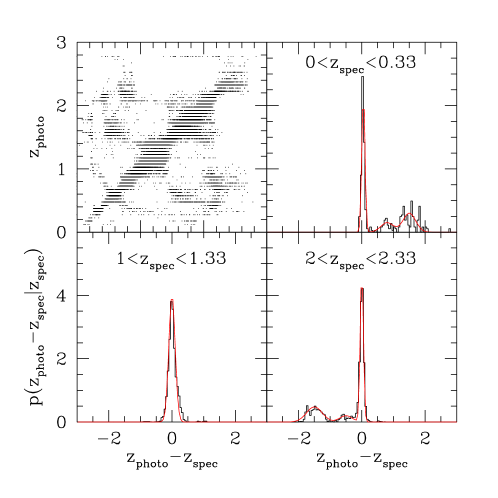
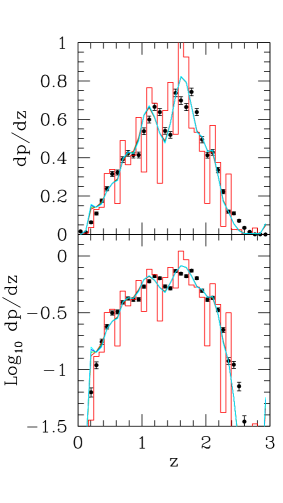
Figure 4: Left: Distribution of spectroscopic and photometric redshifts in the SDSS DR1 NBC QSO catalog. Right: Reconstruction of the intrinsic $dN/dz$ distribution (filled circles) from that of the photometric redshifts (histogram) using the deconvolution algorithm described previously (curve). The reconstruction is quite accurate, despite the complicated nature of the distance errors.

To check that this expression is indeed the correct one, note that maximizing the (log of the) likelihood requires evaluation of $\sum_{i}\partial\,{\rm ln}p_{i}/\partial a$. This reduces to taking the difference of two terms, the first of which is

$$\sum_{i}{\partial\,{\rm ln}N_{e}(\lambda_{i},\zeta_{i},{{\mbox{\boldmath$a$}}})\over\partial a}\to\int{\rm d}\zeta\,\int{\rm d}\lambda{N_{t}(\lambda,\zeta)\over N_{e}(\lambda,\zeta,{{\mbox{\boldmath$a$}}})}{\partial N_{e}(\lambda,\zeta,{{\mbox{\boldmath$a$}}})\over\partial a},$$

where we have written the sum over objects as an integral over their estimated redshifts and luminosities. Similarly, the second term is

$$\sum_{i}{\partial\,{\rm ln}N_{e}(\zeta_{i},{{\mbox{\boldmath$a$}}})\over\partial a}\to\int{\rm d}\zeta\,{N_{t}(\zeta)\over N_{e}(\zeta,{{\mbox{\boldmath$a$}}})}{\partial N_{e}(\zeta,{{\mbox{\boldmath$a$}}})\over\partial a}.$$

Maximizing the likelihood means that we vary $a$ until both these expressions are equal.

Suppose that the true distribution would produce $N_{t}(\lambda,\zeta)$, and that this true distribution is well described by a particular choice of the parameters, say ${{\mbox{\boldmath$a$}}}_{t}$. Then the question is, are the two expressions equal when ${{\mbox{\boldmath$a$}}}={{\mbox{\boldmath$a$}}}_{t}$? If not, our definition of $p_{i}$ is incorrect, because the minimum will occur at some other value of $a$. To see that it is the correct choice, note that when $N_{e}(\lambda,\zeta,{{\mbox{\boldmath$a$}}}_{t})=N_{t}(\lambda,\zeta)$, then the first expression becomes

$$\int{\rm d}\zeta\,\int{\rm d}\lambda{\partial N_{e}(\lambda,\zeta,{{\mbox{\boldmath$a$}}}_{t})\over\partial a}=\int{\rm d}\zeta\,{\partial N_{e}(\zeta,{{\mbox{\boldmath$a$}}}_{t})\over\partial a}.$$

And because

$$N_{e}(\zeta,{{\mbox{\boldmath$a$}}}_{t})=\int{\rm d}\lambda\,N_{e}(\lambda,\zeta,{{\mbox{\boldmath$a$}}}_{t})=\int{\rm d}\lambda\,N_{t}(\lambda,\zeta)=N_{t}(\zeta),$$

the second expression also reduces to $\int{\rm d}\zeta\,{\partial N_{e}(\zeta,{{\mbox{\boldmath$a$}}})/\partial a}$. Thus, both the sums over $i$ reduce to the same quantity. Hence, maximizing the expression for the likelihood given above (equation 15) does indeed yield an accurate unbiased estimate of the luminosity function. This also demonstrates that omission of the ${\rm d}V_{\rm com}$ terms present in our expression for $p_{i}$ would lead to a biased estimate of the shape of the luminosity function.

4 Some applications

4.1 Galaxies and QSOs: $dN/dz$ and $\phi(L)$

The methods above allow one to reconstruct the intrinsic $dN/dz$ and $\phi(L)$ distributions of, e.g., QSOs, LRGs and other galaxy distributions in, e.g., the SDSS. These will be useful for a number of clustering analyses, as well as for studying galaxy evolution. As a proof of concept, Figure 4 shows the result of running the $dN/dz$ deconvolution algorithm on publically available data. The input QSO catalog is from application of the Non-parametric Bayesian Classification algorithm to the SDSS DR1: this produced a catalog of about 100,000 objects (Richards et al. 2004). For each object, photometric redshifts were determined following Weinstein et al. (2004). About 22,000 of these objects have spectra from which a spectroscopic redshift estimate is available. For this subset of objects, the top left panel compares $z_{\rm phot}$ and $z_{\rm spec}$. The other panels show that the distribution of $p(z_{\rm phot}-z_{\rm spec}|z_{\rm spec})$ is rather complex. The panels on the right show the differences between the true- (filled circles) and photo-$z$ distributions (histograms), and that the deconvolution algorithm (curve) does a reasonable job reconstructing the former from the latter.

4.2 Peculiar velocities

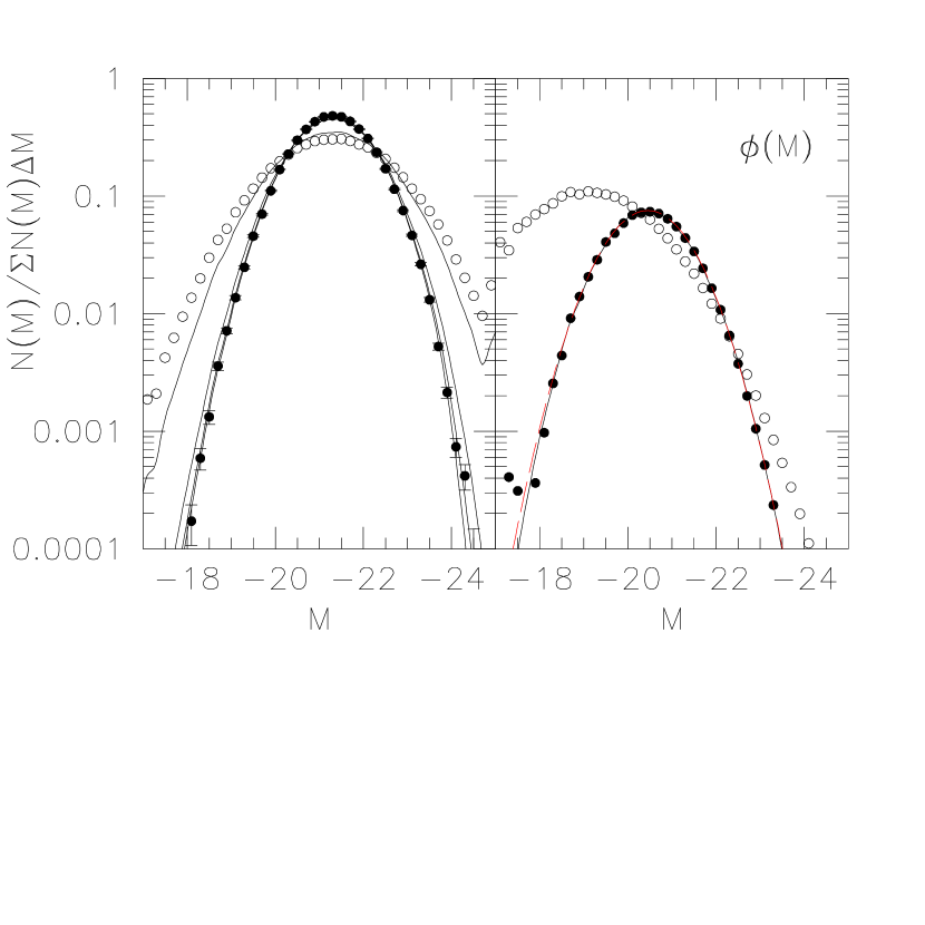
Figure 5: Same as Figure 3, but now the underlying luminosity function is Lognormal (Gaussian in absolute magnitude), and the errors in distance are also assumed to be Lognormal. Parameters were chosen to mimic early-type galaxies in the SDSS (from Bernardi et al. 2003), and distance errors were chosen to be about a factor of two larger than in typical peculiar velocity surveys. Notice how the raw photo-$z$ estimate of $N(M)$ (open circles in panel on left) is broader than the true distribution (filled circles), making the estimated luminosity function have a slight excess of luminous galaxies, and a significantly larger excess of faint galaxies (open circles in panel on right). Nevertheless, when started from the estimated distribution, our deconvolution algorithm quickly converges to the true distribution.

In peculiar velocity surveys such as SFI, ENEAR, EFAR and 6dF, the distance indicator (the Tully-Fisher, $D_{n}-\sigma$, or Fundamental Plane relations) is noisy: typically this noise is approximately twenty percent of the distance, or about 0.4 mags. If uncorrected for, a generic effect of distance uncertainties is to inflate the estimated number of low (and high) luminosity galaxies. This is illustrated in Figure 5, where the error has been set to 1 mag so that the effect is more clearly seen. Since the faint end of the luminosity function provides a strong constraint on galaxy formation models, it is important that it be measured accurately. Therefore, it may be interesting to apply our methods to data from peculiar velocity surveys. In particular, such methods may be necessary for estimating unbiased luminosity functions from HIPASS and ALFALFA.

4.3 The stellar luminosity function

Distances to stars are sometimes estimated by the method of photometric parallax: essentially, this method uses the offset from a color magnitude-relation to infer a distance. Because the color-magnitude relation almost certainly has intrinsic scatter (current estimates are about 0.5 mags), the associated distance estimate is noisy: this is entirely analogous to the noise in distance estimates from peculiar velocity surveys. Determination of the stellar luminosity function is an important ingredient in understanding the IMF. Most current determinations are based on the method of Stobie et al. (1989) which assumes small errors in the distance estimate, and requires prior knowledge of the shape of the luminosity function. Since our non-parametric methods are accurate even when the noise on the distance estimate is large, it may be interesting to apply our methods to this problem as well.

4.4 Correlations between observables

So far, I have mainly discussed how to make accurate estimates of the true redshift and luminosity distributions when only noisy distance estimates are available. However, noisy distance estimates have another important effect for which it is possible to correct. Namely, galaxy observables are known to correlate with one-another: the most well-known of these is the correlation between luminosity $L$ and circular velocity $V_{c}$ (the Tully-Fisher relation for spirals), or velocity dispersion $\sigma$ (the Faber-Jackson relation for ellipticals), but physical size $R$ and surface brightness $I$ are also well-correlated (the Kormendy relation for ellipticals), and $L$ also correlates with size and color for both spirals and ellipticals. Every one of these correlations has been used to constrain galaxy formation models, and, since one measures apparent magnitudes and angular sizes rather than absolute magnitudes and physical sizes, every one of these relations includes at least one distance-dependent quantity.

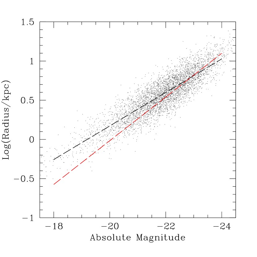
Figure 6: Effect of distance errors on the estimated correlation between size and luminosity for early-type galaxies. Steeper dashed line shows the true $\langle\sigma|L\rangle$ relation, and shallower line shows a least squares fit to the dots which were obtained by using the photo-$z$ estimate of the distance to compute the sizes and absolute magnitudes.

Noise in the distance estimate will lead to biased estimates of these correlations. To illustrate, Figure 6 shows the correlation between luminosity and size in a catalog which is constructed to mimic the SDSS early-type galaxy sample (Bernardi et al. 2003). The steeper dashed curve shows the true $\langle R|L\rangle$ relation. The dots show the result of assuming that $z_{\rm phot}=z_{\rm spec}\ +$ gaussian with rms 0.03 (this amount of scatter in the distance estimate is realistic), and then recomputing the absolute magnitude and size using $z_{\rm phot}$ instead of $z_{\rm spec}$. The shallower dashed line shows $\langle R_{\rm phot}|L_{\rm phot}\rangle$: the change in slope is dramatic.

The qualitative nature of the effect is easy to understand. Distance errors scatter objects towards the bright and faint luminosity tails. This increases the spread along the absolute magnitude axis. If this were the only effect, then one might expect the $R-L$ relation to be shallower. However, the distance error causes a correlated change to the size: assuming an object is closer than it really is makes one infer a smaller luminosity and size than it really has. So the net motion of each point is left-and-down, or right-and-up. If these motions were parallel to the principal axis of the true relation, the net effect would only be to change the scatter of the relation. In this case, they are not, so small distance errors have a non-negligible effect.

This bias is simpler to correct-for when only one of the variables is distance-dependent. For instance, in the case of the $L$-color relation, it is only $L$ which is affected by the distance error (this is not quite true, because $k$-corrections depend on wavelength—I am mainly using this to illustrate an argument). This suggests that if the distance indicator is unbiased in the mean, then the mean $L$ as a function color can be estimated directly. (The scatter around this mean relation is interesting in its own right: it will, of course, be affected by the noise in the distance estimate.) In practice, however, even this case is not entirely straightforward, because galaxy catalogs are almost always magnitude limited, and this introduces selection effects into the estimate of $\langle L|{\rm color}\rangle$; absent distance errors, it is $\langle{\rm color}|L\rangle$ rather than $\langle L|{\rm color}\rangle$ which can be estimated free of selection effects! When accurate distances are known, these selection effects can be accounted for by using the quantity $V_{\rm max}$ which played an important role in our discussion of the luminosity function. This suggests that the methods discussed previously should allow one to estimate such correlations in photometric galaxy catalogs. When the distance error appears in both variables, it is slightly harder to correct, but a correction is still possible. Essentially, one simply needs to write the expressions given previously in matrix rather than scalar notation. Making this generalization correctly is the subject of work in progress.

5 Discussion

I presented two algorithms for estimating the intrinsic redshift and luminosity distributions from photo-$z$ surveys. These algorithms improve on previous work by Subbarao et al. (1996) and Chen et al. (2003). Subbarao et al. concluded that numerical simulations were necessary to derive accurate estimates—my analysis shows that simulations can be avoided. Chen et al. wrote down a maximum likelihood expression which they then maximized—I find a different expression for the likelihood, and provide an analytic calculation which shows that maximizing this expression does indeed lead to an unbiased estimate; maximizing their expression instead would return a biased answer.

The error in the photometric redshift gives rise to an error in the estimated luminosity. Since measurement errors in the apparent magnitude also give rise to errors in the estimated luminosity, it is tempting to treat the photo-$z$ errors similarly to how one treats the effects of errors in the photometry. However, the two errors are not equivalent for the simple but important reason that the photo-$z$ error, while affecting the estimated luminosity, leaves the observed apparent magnitude unchanged. In this respect, it is more accurate to view the photo-$z$ error as equivalent to a peculiar velocity. This motivates reanalysis of relatively shallow galaxy surveys for which the peculiar velocity may be a substantial fraction of the observed redshift, e.g. faint, nearby, low surface brightness galaxies, or galaxies in the 6dF survey (Jones et al. 2004). In this case, the error in the true distance comes from the thickness of the Fundamental Plane, or the $D_{n}-\sigma$ relation, and is typically on the order of twenty percent.

The fractional error on the distances to most stars in our galaxy (those for which parallax measurements are not available) is relatively large. Stobie, Ishada & Peacock (1989) discuss a method for estimating the luminosity function in the case of photometric parallaxes derived from the color-magnitude relation, but the approach is parametric (it requires an accurate guess of the intrinsic shape of the luminosity function), and it assumes that the distance errors are small. Our approach provides accurate non-parametric estimates which are valid even when the errors are large. We intend to apply our methods to provide non-parametric estimates of the stellar luminosity function which are not compromised by the noise in the distance estimator.

Both the maximum likelihood and the $V_{\rm max}$ estimators I derived assume that galaxies do not evolve, so one must break the sample up into narrow redshift bins before analysis. This is risky in principle, because one wants a narrow bin in true redshift, but only photo-$z$s are available. In practice, photo-$z$s are sufficiently accurate that a narrow bin in photo-$z$ is still quite narrow in true-$z$. The maximum-likelihood and $V_{\rm max}$ estimators of the luminosity function have another drawback: they ignore the fact that different galaxy types require different $k(z)$-corrections, so one must preselect the sample to insure that it contains galaxies that are of the same type. Extending the analysis to allow for evolution and type is clearly desirable, and is the subject of work in progress.

References

- [1] Bernardi M., Sheth R. K., Annis J., et al., 2003, AJ, 125, 1849
- [2] Bolzonella M., Miralles J.-M., Pello R., 2000, AA, 363, 476
- [3] Cabre A., Gaztanaga E., Manera M., Fosalba P., Castander F., 2006, MNRAS, 372, 23
- [4] Chen H.-W., Marzke R. O., McCarthy P. J., Martini P., Carlberg R. G., Persson S. E., Bunker A., Bridge C. R., Abraham, R. G., 2003, ApJ, 586, 745
- [5] Collister A., Lahav O., 2004, PASP, 116, 345
- [6] Collister A., Lahav O., Blake C., et al., 2007, MNRAS, tmp.1478C
- [7] Connolly A. J., Csabai I., Szalay A. S., Koo D. C., Kron R. C., Munn J. A., 1995, AJ, 110, 2655
- [8] Efstathiou G., Ellis R. S., Peterson B. A., 1988, MNRAS, 232, 431
- [9] Eisenstein D. J., Annis J., Gunn J. E., et al., AJ, 122, 2267
- [10] Fosalba P., Gaztanaga E., Castander F., 2003, ApJ, 597, 89
- [11] Jones et al., 2004, MNRAS, 355, 747
- [12] Lucy L. B., 1974, AJ, 79, 745
- [13] Marchesini D., van Dokkum P., Quadri R., Rudnick G., Franx M., Lira P., Wuyts S., Gawiser E., Christlein D., Toft S., ApJ, in press (astro-ph/0610484)
- [14] Padmanabhan N., Budavari T., Schlegel D. J., et al., 2005, MNRAS, 359, 237
- [15] Padmanabhan N., Hirata C. M., Seljak U., Schlegel D. J., Brinkmann J., Schneider D. P., 2005, PRD, 72, 043525
- [16] Richards G. T., Nichol R. C., Gray A. G., et al., 2004, ApJS, 155, 257
- [17] Sandage A., Tammann G., Yahil A., 1979, ApJ, 232, 352
- [18] Schmidt M., 1968, ApJ, 151, 393
- [19] Scranton R., Menard B., Richards G. T., et al., 2005, ApJ, 633, 589
- [20] Scranton R., Connolly A. J., Nichol R. C., et al., 2003, PRL, submitted (astro-ph/0307335)
- [21] Springel V., White S. D. M., 1998, MNRAS, 298, 143
- [22] Stobie R. S., Ishida K., Peacock J. A., MNRAS, 1989, 238, 709
- [23] Subbarao M. U., Connolly A. J., Szalay A. S., 1996, AJ, 112, 929
- [24] Weinstein M A., Richards G. T., Schneider D. P., et al., 2004, ApJS, 115, 243
- [25] Wolf C., Meisenheimer K., Rix H.-W., Borch A., Dye S., Kleinheinrich M., 2003, AA, 401, 73
- [26] York D., et al., 2000, AJ, 120, 1579