Detectability of Occultation of Stars by Objects in the Kuiper Belt and Oort Cloud

Abstract

The serendipitous detection of stellar occultations by Outer Solar System objects is a powerful method for ascertaining the small end ($r\lesssim 15$ km) of the size distribution of Kuiper Belt Objects and may potentially allow the exploration of objects as far out as the Oort Cloud. The design and implementation of an occultation survey is aided by a detailed understanding of how diffraction and observational parameters affect the detection of occultation events. In this study, stellar occultations are simulated, accounting for diffraction effects, finite source sizes, finite bandwidths, stellar spectra, sampling, and signal-to-noise. Finally, the possibility of detecting small Outer Solar System objects from the Kuiper Belt all the way out to the Oort Cloud is explored for three photometric systems: a proposed space telescope, Whipple (Kaplan et al., 2003), the Taiwanese-American Occultation Survey (Lehner et al., 2006), and the Multi Mirror Telescope (Bianco, 2007).

1 Introduction

Stellar occultation, the dimming of a background star by a foreground object passing through the line of sight, is used in a variety of scientific studies to probe the properties of foreground objects. With stellar occultations, it has been possible to discover and study planetary rings (e.g. Bosh et al., 2002, references therein) and the atmospheres of planets and their satellites (e.g. Elliot et al., 2003a, b; Gulbis et al., 2006; Pasachoff et al., 2005; Sicardy et al., 2006).

Studies suggest that by searching for serendipitous occultations in monitored stars it may be possible to detect Outer Solar Systems objects in the Kuiper Belt (Dyson, 1992; Axelrod et al., 1992) and objects as far out as the inner edge of the Oort Cloud (Bailey, 1976). This provides a novel way to ascertain the size distribution of small object populations in the Kuiper Belt and the Inner Oort Cloud.

The standard planet formation scenario begins with a disk of small planetesimals (with radii $r<0.5$ km) surrounding a protostar. These planetesimals collide with one another and merge to become larger objects. When sufficiently massive, gravitational focusing leads to runaway accretion. Larger objects dominate the accretion process and eventually go on to become planets. Remaining planetesimals, by a variety of mechanisms, are cleared from the planet region of the disk. Some objects are ejected to distant orbits by perturbations from the giant planets. At the outer edge of the protostellar disk, a slow rate of collision fails to produce large enough objects and planet formation fails to occur. Far enough removed from the massive planets, these smaller planetesimals are invulnerable to perturbations and remain in the disk.

In our own Solar System, the Kuiper Belt is a remnant of the outer protostellar disk which failed to form planets. The population of planetesimals in this region have most likely been perturbed by Neptune and perhaps other massive bodies, therefore the Kuiper Belt’s size distribution, spatial distribution, and mass are important keys to understanding the evolution of planetary disks.

Models and observations suggest the differential size distribution of the Kuiper Belt follows a broken power law $N\propto r^{-q}$, where $q$ takes on different values in the lower and upper size regions. The location of the break $r_{\mathrm{b}}$ in this power law depends on the initial mass, size spectrum, and bulk properties of Kuiper Belt Objects (KBOs), and Neptune’s orbital evolution among other parameters (Kenyon & Bromley, 2004; Kenyon, 2002; Pan & Sari, 2005; Stern, 1996). Observations have constrained the size spectrum for large objects ($r\gtrsim 100$ km) to an index $q\sim 4$ (Bernstein et al., 2004; Trujillo et al., 2001). Bernstein et al. (2004) has found evidence for a break in the size distribution near $r_{\mathrm{b}}\sim 30$–50 km by a faint object survey mounted on the Advanced Camera for Surveys (ACS) on the Hubble Space Telescope (HST). Previous models predicted the location of the break radius at $0.05~{}\mathrm{km}<r_{\mathrm{b}}<5~{}\mathrm{km}$ (Stern, 1996; Kenyon & Luu, 1999; Kenyon, 2002). Kenyon & Bromley (2004) and Pan & Sari (2005) have since modeled the Kuiper Belt size distribution revisiting assumptions made about the relative gravitational and tensile energies of KBOs. Pan & Sari (2005) concluded that bulk strength plays little role in the fragmentation of small objects and find reasonable agreement with the suggested break location evidenced by Bernstein et al. (2004). Kenyon & Bromley (2004) estimated the break radius at $0.5~{}\mathrm{km}<r_{\mathrm{b}}<15~{}\mathrm{km}$. Additionally they suggested that a dip should be present at $5<r<35$ km due to the removal of small objects due to collisional erosion. These two models differ in the small size range where direct observations are difficult due to the dim surface brightness of KBOs smaller than $r=15$ km.

Surveys monitoring background stars for occultations due to KBOs have the capability to determine the small end of the KBO size distribution (Roques & Moncuquet, 2000; Cooray & Farmer, 2003). Various groups are now attempting to implement such surveys (e.g. Roques et al., 2003; Bickerton, 2006; Lehner et al., 2006; Chang et al., 2006). Roques et al. (2003) have implemented a survey at the Pic du Midi Observatory with sampling at 20 Hz frequency. They reported a candidate event at $3\sigma$ which may be ascribed to an occultation by a $r\sim 0.15$ km KBO. Three candidate occultation events were also reported by a later survey conducted with a frame transfer camera mounted on the 4.2 m William Herschel Telescope at La Palma (observing at 46 Hz) (Roques et al., 2006). However, the survey team ruled out the detection of any KBOs in the $30$–50 AU range. Bickerton (2006) have also followed suit by implementing a high-speed CCD camera design with 40 Hz cadence and mounting a search with the 72-inch Plaskett telescope in Victoria, BC. Additionally, King et al. (2002) and Lehner et al. (2006) have described a dedicated occultation survey known as The Taiwanese-American Occultation Survey (TAOS) which uses three wide-field robotic telescopes to monitor as many as 2,000 stars for chance occultations by KBOs.

Recently, candidate occultation events at millisecond timescales were observed in X-ray lightcurves of Scorpius X-1 (Chang et al., 2006). These events were claimed to be compatible with KBOs in the size range $5~{}\mathrm{m}<r<100~{}\mathrm{m}$. The reported event rate is much higher than expected from models of KBO formation. Jones et al. (2006) have argued that the candidate events observed by Chang et al. (2006) are attributed to dead time response due to charged particle scintillation. Subsequently, Chang et al. (2007) adjusted their number of candidate occultation events to account for this effect. To date, occultation surveys have been unable to provide definite constraints on the small size distribution of objects in the Kuiper Belt.

Beyond the Kuiper Belt, there remain many questions that could be addressed by stellar occultation surveys. The structure of the Outer Solar System is thought to extend from the Kuiper Belt out to distances as large as $\sim 100,000$ AU. The nature of this vast region holds important clues to the complex evolution of our Solar System.

The Oort Cloud is a population of planetesimals that is thought to have been scattered from the planetary disk roughly $\sim 4.5$ Gyr ago, and is predicted to have a wide range of orbits with semi-major axes spanning distances of $1,000~{}\mathrm{AU}<a<100,000~{}\mathrm{AU}$. Its existence was proposed as a probable reservoir of long-period comets (Oort, 1950).

Models suggest that these objects formed in the region of the giant planets ($\sim 4-40$ AU) and were perturbed by the giant planets to large orbits with relatively unchanged perihelia. Interactions with nearby passing stars, giant molecular clouds, and other material in the solar neighborhood would have increased their perihelia to larger distances, increased the inclinations, and placed them in large orbits to form the Oort Cloud (Dones et al., 2004). Dynamical simulations combined with the flux of long-period comets into the planetary region of the Solar System lead to estimates of the number of comets in the Oort Cloud to be $\sim 10^{11}-10^{12}$. However, because the Oort Cloud is at such large distances and its comets are expected to be the size of observed long-period comet nuclei ($r\sim 3$ km), direct observations of the Oort Cloud are unlikely.

The discovery of Sedna (2003 VB12), a $r=830$ km object on an eccentric orbit at heliocentric semi-major axis of $a=490$ AU, came as a surprise (Brown et al., 2004). An object of substantial size at such a distant orbit was unexpected. Sedna’s origins remain unclear, but its discoverers (Brown et al., 2004) have suggested that Sedna may be part of the Oort Cloud. This implies that Sedna amassed size in the planetary region and was perturbed to its current orbit (Morbidelli & Levison, 2004; Matese et al., 2005). Stern (2005) has pointed out that Sedna’s eccentric and inclined orbit does not preclude its formation in situ. If this is true, it is possible that Sedna is part of a population of objects that lie in a proposed annular region beyond the Kuiper Belt (Brasser et al., 2006) which is referred to in this paper as the Extended Disk ($a\sim 50$–1,000 AU).

Using stellar occultations to search for Extended Disk objects is also a possibility. To date, no known occultation surveys are dedicated to this purpose. However, Roques et al. (2006) showed that this may be a real possibility as they identified two candidate occultation events by 300 m radius objects beyond 100 AU via this method.

The potential for occultation surveys to detect objects in the Kuiper Belt is well discussed in the literature. However, the capability of a given occultation survey to detect objects out to the Oort Cloud still requires careful consideration as it depends on several factors. In particular, Roques & Moncuquet (2000) have shown that star light diffraction must be taken into account for surveys looking to detect stellar occultations by small objects in the Kuiper Belt. In this paper, the effects of stellar types, finite bandwidth and sampling on a survey’s ability to detect occultation events in the Outer Solar System are studied. Occultation events for three photometric systems are simulated in order to guide the selection of observational parameters for occultation surveys. In § 2 a brief introduction to stellar occultation and diffraction effects are given. The effects of finite bandwidth, stellar spectra, and finite source sizes are considered later in § 3. The effects of sampling is discussed in § 4. Noise for three photometric systems as mentioned above is included in § 5. Finally, the detectability of an occultation event for photometric systems and the conclusions of this study are discussed in § 6, § 7, and § 8.

2 Stellar Occultations and Diffraction

The diffraction pattern created by the stellar occultation of a distant star by a foreground spherical object is described using Lommel functions,

$$U_{n}(\mu,\nu)=\sum\limits^{\infty}_{k=0}\left(-1\right)^{k}\left(\frac{\mu}{\nu}\right)^{n+2k}J_{n+2k}(\pi\mu\nu),$$

where $J_{n}$ is a Bessel function of order $n$. For the case of an occultation by an object of radius $r$ at a distance $a$, the measured intensity of a star at wavelength $\lambda$ is described (Roques et al., 1987, and references therein) by

$$I_{\rho}(\eta)\!=\!\left\{\!\!\begin{array}[]{ll}U_{0}^{2}(\rho,\eta)+U_{1}^{2}(\rho,\eta)\vspace{0.05in}&\eta\leq\rho\vspace{0.05in}\\ 1+U_{1}^{2}(\rho,\eta)+U_{2}^{2}(\rho,\eta)&\eta\geq\rho\\ \>-2U_{1}(\rho,\eta)\sin\frac{\pi}{2}(\rho^{2}+\eta^{2})&\\ \>+2U_{2}(\rho,\eta)\cos\frac{\pi}{2}(\rho^{2}+\eta^{2})&\end{array}\right.,$$ (5)

where $\rho=r/F$ and $\eta=x/F$ are the radius and distance from the line of sight in units of the Fresnel scale $F=\sqrt{\lambda a/2}$. The subscript on $I_{\rho}$ indicates that the occultation pattern depends solely on the dimensionless parameter $\rho$.

Figure 1 shows a projected occultation pattern computed from the above expression for $\rho=1.0$. Also shown are four trajectories through the occultation pattern at four different values of the impact parameter $b$, given in terms of the diameter of the first Airy ring (this is an approximate definition as will be discussed further), which we will call $\Omega$. The corresponding intensity profile curves for each of these trajectories are shown in Figure 2. An object crossing a source with a finite impact parameter leads to several possible intensity curves for a given occultation pattern. From the plots shown in Figure 2, it can be seen that for impact parameters $b\geq 0.5\Omega$, the occultation event depth is quite small, and such events will be very difficult to detect. We thus define an occultation event as an object crossing the line of sight to a star with an impact parameter $b\leq 0.5\Omega$, and we define the event width as the first Airy ring diameter $\Omega$. Finite impact parameters complicate the characterization of an occultation event because of the multitude of possible intensity curves that may arise from one occultation pattern. In order to simplify the discussion, only the case of $b=0$ is considered throughout the remainder of this paper. This assumption does not significantly alter the conclusions.

Note that at center of the diffraction pattern in Figure 1, $I_{\rho}(0)=1$; this is the Poisson spot and is a consequence of diffraction present for circular objects passing before a point source.

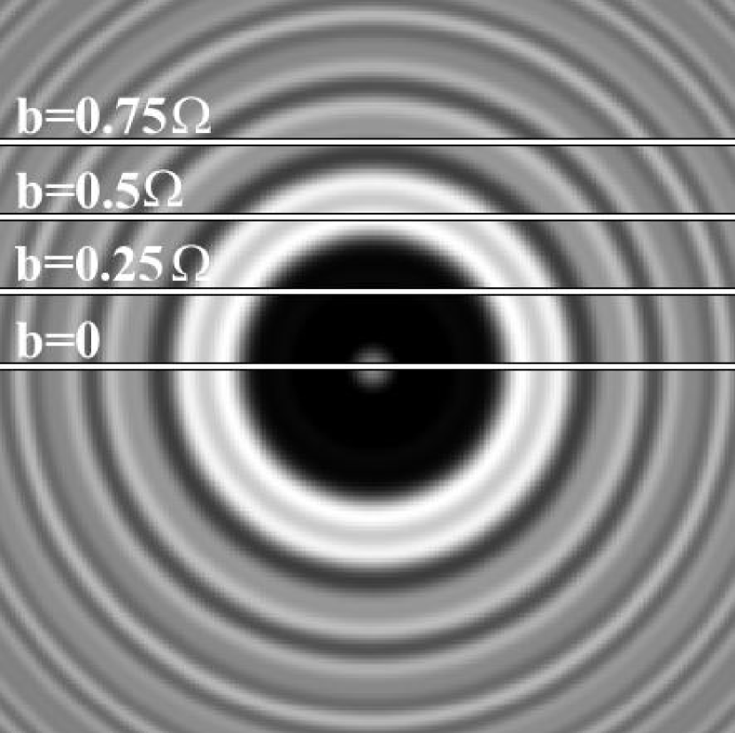
Figure 1: The projected occultation pattern for $\rho=1$. The scale of the pattern is 5 Fresnel units on a side. Four trajectories crossing the occultation pattern with impact parameters $b$ are shown with corresponding intensity curves in Figure 2. Values for the impact parameters are expressed in terms of the occultation width $\Omega$ shown in Figure 2.

Figure 2: Intensity curves for an occultation pattern for $\rho=1$ traversed at various impact parameters $b$. Impact parameter values are labeled at the bottom of each plot and correspond to their labeled counterparts in Figure 1.

The parameter $\rho$ defines the strength of diffraction effects, in particular the width and depth of the occultation. Assuming a point source background star, the occultation width $\Omega$ (see Figure 2) takes on two values in the limiting cases of large and small $\rho$. For $\rho\ll 1$, the occultation pattern is completely dominated by diffraction and the diameter of the Airy ring is given by $2\sqrt{3}$ in dimensionless Fresnel scale units. In the case where $\rho\gg 1$, the diffraction effects become negligible and the width approaches the limiting case of $2\rho$. An empirical approximation over the entire region of interest is given by

$$\Omega\approx 2\left[\left(\sqrt{3}\right)^{3\over 2}+\rho^{3\over 2}\right]^{{2\over 3}}.$$ (6)

In physical units, the width $W$ is

$$W\approx 2\left[\left(\sqrt{3}F\right)^{3\over 2}+r^{3\over 2}\right]^{{2\over 3}}.$$ (7)

Figure 3 shows the measured width (solid line) against the approximation in Equation 6 (dashed line). The two limiting expressions for large and small $\rho$ are indicated by dotted-lines. The “jumps” in occultation width $\Omega$ for $0.3\lesssim\rho\lesssim 9$ are the result of the gradual shifting of diffraction fringes near the shadow edge. Figure 4 depicts three lightcurves near $\rho\sim 1$ ($\rho=0.98$, 1.00, and 1.02). Determining the maximum peak is complicated by diffraction fringes that span the shadow edge. The jumps in the event width are due to one of two local maxima becoming larger than the other. The measured width for each of the curves are depicted in Figure 4 by vertical lines drawn to match the appropriate curve.

Figure 3: Occultation width $\Omega$ (see Figure 2) versus the object radius $\rho$. The solid line shows the measured width, the dotted line shows the approximation given in Equation 6, and the dashed lines indicate the asymptotic behavior for $\Omega$ in the two limiting cases for $\rho$.

Figure 4: Occultation patterns for $\rho=0.98$, 1.00, and 1.02. Vertical lines indicate the measured widths for each pattern. Increases in $\rho$ shift the absolute maximum peak by a significant amount.

For a source of finite angular radius $\theta_{\ast}$, the projected radius in the plane of the occulting object is $r_{\ast}=a\theta_{\ast}$. This finite radius extends the occultation width by the projected diameter of the star such that

$$\Omega^{\ast}\approx 2\left[\left(\sqrt{3}\right)^{3\over 2}+\rho^{3\over 2}\right]^{{2\over 3}}+2\rho_{\ast},$$ (8)

where $\rho_{\ast}=r_{\ast}/F$, and the asterisk in the superscript indicates that a finite source disk is accounted for in the occultation width. The width in physical units is thus

$$W^{\ast}\approx 2\left[\left(\sqrt{3}F\right)^{3\over 2}+r^{3\over 2}\right]^{{2\over 3}}+2r_{\ast}.$$ (9)

The occultation depth $\Delta$ is defined as the magnitude of the maximum downward deviation of an occultation pattern, as drawn in Figure 2. Figure 5 is a plot of the depth $\Delta$ as a function of $\rho$. There are two limiting cases of the occultation depth as a function of $\rho$. An empirical fit to $\Delta(\rho)$ for $\rho\ll 1$ shows that the depth roughly follows a power law $\Delta\approx 3\rho^{2}$. In the limit where $\rho\gg 1$, the object disk completely extinguishes the background source, hence the depth is constant at $\Delta=1$. By an empirical fit to the measured depth, we arrive at the expression

$$\Delta=\left[1+\left(3\rho^{2}\right)^{-{3\over 2}}\right]^{-{2\over 3}}$$ (10)

Figure 5: Occultation event depth $\Delta$ (see Figure 2), as function of $\rho$. The solid line shows the measured depth, the dashed line shows the empirical approximation in Equation 10, and the dotted lines show the two limiting cases.

Three regimes are apparent in Figures 3 & 5: (1) the far-field or Fraunhofer regime for $\rho\ll 1$, (2) the near-field or Fresnel regime for $\rho\sim 1$, and (3) the geometric regime for $\rho\gg 1$. In the Fraunhofer regime the occultation width $\Omega=2\sqrt{3}$ is independent of $\rho$, but the depth varies as $\Delta\approx 3\rho^{2}$. Example diffraction patterns in this regime are shown in Figure 6 for the cases $\rho=0.03$, $0.01$, and $0.3$. It is clearly evident in this figure that as $\rho$ decreases, the width remains constant and the depth decreases. In the Fresnel regime the depth and width of the occultation event are both dependent on $\rho$, hence as $\rho$ increases both parameters will increase as seen in Figure 6 where $\rho=1.0$, and $3.0$. Finally, geometric patterns have a width which approaches the geometric shadow $\Omega\to 2\rho$ and complete extinction of the background source is apparent such that $\Delta=1$. Figure 6 shows an occultation event approaching the geometric regime in the panel for $\rho=9.0$.

Figure 6: Occultation intensity profiles measured across the center of the pattern for several values of $\rho$.

3 Spectral Type and Finite Size of Source Star

Occultation patterns described in the previous section depend upon the observation wavelength $\lambda$. In reality, a survey will monitor stars through a finite bandwidth and this can affect the diffraction features observed in an occultation pattern. If the bandwidth is narrow, a monochromatic pattern is a reasonable approximation for an observed occultation. For broader bandwidths like that of TAOS, we describe the intensity pattern as

$$I_{r,a}(x)=\int\limits^{\infty}_{-\infty}s(\lambda)f(\lambda)I_{r,a}(x,\lambda)d\lambda,$$ (11)

where

$$I_{r,a}(x,\lambda) = I_{\rho}(\eta)$$

$$= I_{r/F(a,\lambda)}(x/F(a,\lambda)),$$

and the wavelength-dependent filter transmission and stellar spectrum are represented by $f(\lambda)$ and $s(\lambda)$ respectively.

To determine broad bandwidth effects, $I_{r,a}(x,\lambda)$ for several $r$ and $a$ were integrated against a flat spectrum with a series of tophat filters. Stellar spectra were accounted for using the UVILIB library, a compiled stellar flux library spanning a total wavelength range of 1,150–10,620 Å (Pickles, 1998), was incorporated into occultation curve simulations. We found that for point sources broader bandwidths will smooth and dampen diffraction fringes, while broadening of the occultation width is minimally seen. Additionally, stellar spectra appear to have little effect on the intensity profile of a diffraction pattern for a background point source.

Throughout the remainder of this paper, the Fresnel scale of an event with a broadband filter is redefined as

$$F=\sqrt{\bar{\lambda}a\over 2},$$

where $\bar{\lambda}$ is the median wavelength of the filter of interest.

While the stellar spectra themselves have a minimal effect, finite source sizes will significantly affect the occultation intensity patterns, specifically when $\rho_{\ast}\gtrsim 1$. The source size of a given star is determined by a combination of its stellar class and apparent brightness. To address finite source size effects, stellar radii from tabulated values (Cox, 2000; Lang, 1992) were incorporated into simulations of occultation events. (Limb darkening effects also were considered using a solar limb darkening model (Cox, 2000), however the effects were found to be $\lesssim 1$%, hence they are ignored throughout the rest of this discussion.)

The intensity profile from a finite source disk of projected radius $r_{\ast}$ is expressed as an integral over the projected source disk

$$I_{r,a}^{\ast}(x) = \frac{1}{\pi r^{2}_{\ast}}\int\limits^{2\pi}_{0}\int\limits_{0}^{r_{\ast}}\left(r^{\prime}_{\ast}dr^{\prime}_{\ast}d\phi\right.$$

$$\times \left.I_{r,a}(x^{2}+r^{\prime 2}_{\ast}+2xr^{\prime}_{\ast}\cos\phi)\right).$$

Here $r^{\prime}_{\ast}$ and $\phi$ are the distance from the center of the source disk and the polar angle. The asterisk in the superscript $I^{\ast}$ denotes that the occultation pattern was calculated accounting for the finite source size.

Occultation profiles for four stellar types each with magnitude $V=12$ for $r=0.5$ and 1.5 km objects are plotted in Figures 7 & 8. Both illustrate that the finite source size of a stellar disk can significantly broaden the occultation width and smooth the diffraction fringes. In cases where the source size is relatively large such as an M2V $V=12$ star, the smoothing is so significant that diffraction fringes with variations as large as $\sim$35% are reduced to variations of $\sim$5%.

Figure 7: Diffraction profiles for a KBO for different $V=12$ background stars: A0V, G5V, K5III, and M2V. The occulting object for this set of curves has a radius of 0.5 km and is at a distance of 40 AU. Projected stellar radii at 40 AU are 0.2, 0.5, 1.2, and 2.6 km respectively.

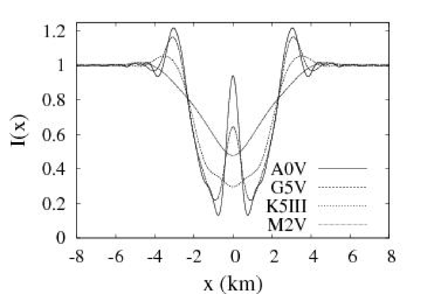
Figure 8: Diffraction profiles for a KBO for different $V=12$ background stars: A0V, G5V, K5III, and M2V. The occulting object for this set of curves has a radius of 1.5 km and is at a distance 40 AU. Projected stellar radii at 40 AU are 0.2, 0.5, 1.2, and 2.6 km respectively.

The smoothing and broadening effects at distances well beyond the Kuiper Belt are more drastic as is expected due to the dependence of the projected source size on the distance $a$. Occultation patterns were calculated for four $V=12$ background source stars for a $r=5$ km Extended Disk object at $a=1,000$ AU (Figure 9) and for a $r=10$ km Oort Cloud object $a=10,000$ AU (Figure 10). These objects are detectable with the A0V star, but they would be extremely difficult to detect with the K5III or M2V stars because of the very small occultation depth due to the large projected radius of the source star.

Figure 9: Diffraction profiles for an Extended Disk object for different $V=12$ background stars: A0V, G5V, K5III, and M2V. The occulting object for this set of curves has a radius of 5 km and is at a distance of 1,000 AU. Projected stellar radii at 1,000 AU are 4.3, 12.9, 30.6, and 64.1 km respectively.

Figure 10: Diffraction profiles for an Oort Cloud object for different $V=12$ background stars: A0V, G5V, K5III, and M2V. The occulting object for this set of curves has a radius of 10 km and is at a distance of 10,000 AU. Projected stellar radii at 10,000 AU are 43.5, 129.4, 306.3, and 641.4 km respectively.

The angular size of a star depends not only on its spectral type, but on its magnitude as well. Figure 11 shows the smoothing effects due to various stellar brightnesses ($V=8$, 10, 12, and 14) for an A0V star occulted by a $r=1.5$ km object at 40 AU. The stellar radii projected into the plane of the object are 1.1, 0.44, 0.17, and 0.069 km, respectively. The change in radius from a 14th to 10th magnitude A0V star will dampen the Poisson peak by $\sim 30$%. However, overall smoothing due to the increase in stellar radius with brightness is minimal for this range. In the case of a $V=8$ A0V star which has a projected source radius comparable to both the Fresnel scale and object radius, the smoothing is significant enough to eliminate any trace of the Poisson peak and most of the other diffraction features.

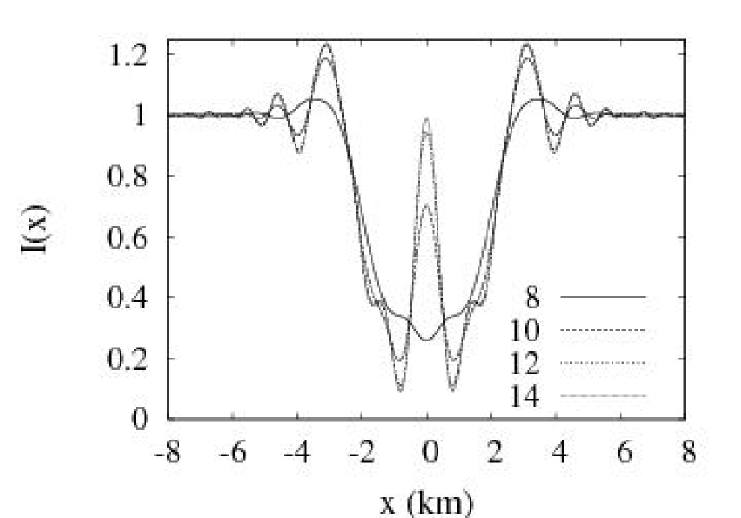
Figure 11: Diffraction profiles for background A0V stars of varying magnitudes: $V=8$, 10, 12, and 14. The lower right-hand key lists V-magnitude values for each curve. Apparent stellar radii at 40 AU are 1.1, 0.44, 0.17, and 0.069 km respectively.

Occultation patterns for stars of various types and brightnesses, and for objects of various sizes and distances, exhibit a wide range in morphologies as can be seen from the previously discussed figures. A summary of the expected occultation pattern morphologies is presented in a plot of object radius $r$ versus distance $a$ (Figure 12) with accompanying example occultation patterns (Figure 13). As described above, the occultation pattern depends upon the projected source size $r_{\ast}$ relative to the Fresnel scale $F$. The morphologies are then split into five regions labeled A, B, C, D, and E. Regions A and D lie in the distance range $a\lesssim 2,000$ AU where the projected source radius $\rho_{\ast}<1$. Conversely, regions B and C lie in the distance range $a\gtrsim 2,000\rm{\ AU}$ where $\rho_{\ast}>1$. Region E lies in the parameter space $\rho_{\ast}\sim 1$.

Figure 12: Plot summarizing resulting lightcurve classes for object radii $r$ and distances $a$ passing before a $V=12$ A0V star. Each class is associated with a region demarcated by the drawn lines and is labeled accordingly (A, B, C, D, and E). Characteristic curve shapes are dependent upon stellar disk radius $r_{\ast}$ (solid line) and the Fresnel scale $F$ (dotted - dashed line). Exemplary curves for each of the listed regions are shown in Figure 13.

Figure 13: Plots of example lightcurves for each of the five morphologies shown in Figure 13. Each curve is labeled with it’s corresponding region.

Recall that when $\rho\gg 1$, the occultation pattern for a point source can be approximated by a geometric shadow. The A and B regions therefore represent the area of the parameter space for geometric occultation patterns. The difference between the two arises from the source size $\rho_{\ast}$. At large distances where $\rho_{\ast}\gtrsim 1$ (region B), significant smoothing by the stellar source disk washes out all diffraction details including the Poisson peak. To contrast, diffraction features remain in the geometric occultation pattern when $\rho_{\ast}\lesssim 1$ (region A).

Occultation patterns which fall into regions C and D in Figure 12 fall within the Fresnel and Fraunhofer regimes ($\rho\lesssim 1$). They both exhibit shallower occultation depths, but again, depending on the source size $\rho_{\ast}$, the occultation will exhibit differing occultation width broadening and smoothing. In region C, the Fresnel scale is smaller than the projected source size, and therefore only a fraction of the stellar flux is diffracted. These events are wide but extremely shallow. Occultation patterns in Region D simply resemble the Fraunhofer patterns we discussed previously because the small source sizes here have little effect. Finally, patterns in region E, where $\rho_{\ast}\sim 1$ and $\rho\sim 1$ , show a significant depth without complete extinction of the source, and are devoid of significant diffraction features.

From the above discussion, it follows that in order to minimize smoothing and maximize the occultation depths, selected target stars should be relatively dim and blue, since brighter and redder stars have larger apparent disks. With this choice a survey would have to contend with reduced signal-to-noise. With better photometry, improved signal-to-noise augmented by brighter background sources may slightly increase the detection of smaller objects as the occultation event widths are extended by the stellar disk (see Equations 8 and 9). This approach however, would sacrifice diffraction details and diminish the depths of occultation events. Background source selection is furthermore complicated by the linear dependence of the projected source radius $r_{\ast}$ on $a$. Effective selection of target stars therefore depends on considerations such as the target population, observational parameters, and expected event rates, as well as lightcurve shape.

4 Relative Velocity and Sampling

Rather than observing stationary occultation patterns like the ones that have so far been discussed, real surveys will observe these patterns in time due to the relative velocity of the object transverse to the line of sight. The main source of the transverse motion is the orbital motion of the Earth, with a small contribution from the velocity of the occulting object itself. Assuming that the occulting object lies in the ecliptic plane on a circular orbit the transverse velocity expression is

$$v_{\mathrm{T}}=v_{\mathrm{E}}\left(\cos\phi-\sqrt{\frac{a_{\mathrm{E}}}{a}\left(1-\frac{a^{2}_{\mathrm{E}}}{a^{2}}\sin^{2}\phi\right)}\right),$$ (12)

where $\phi$ is the angle of opposition, the angle between the object and the opposing direction of the sun, $v_{\mathrm{E}}=29.8$ km s^-1, is the orbital speed of Earth, and $a_{\mathrm{E}}=1$ AU is the distance from the Sun to the Earth. At opposition ($\phi=0^{\circ}$) where the transverse velocity reaches a maximum, the expression for $v_{\mathrm{T}}$ simplifies to

$$v_{\mathrm{T}}=v_{\mathrm{E}}\left(1-\sqrt{\frac{1\rm{\ AU}}{a}}\right).$$ (13)

A typical KBO at a distance of $a=40$ AU will have a transverse velocity $v_{\mathrm{T}}\approx 25$ km s^-1. The occultation profile is then measured as a lightcurve in time $t=x/v_{\mathrm{T}}$. Given the occultation width (see Equation 9), the occultation has a duration

$$T=\frac{W^{\ast}}{v_{\mathrm{T}}}.$$ (14)

A true survey will collect images by temporally integrating infinitesimally sampled lightcurves over a finite exposure time $\Delta t$. Shutter speed, frame transfer, and other photometric delays will lead to time lags between images. However, here we assume that any delays that arise from the photometric system are minimal and that the exposure time is equal to the inverse of the sampling frequency $f=1/\Delta t$. The discrete lightcurve is then given by points integrated in time

$$I(t_{i})=\int\limits_{t_{i}-\Delta t/2}^{t_{i}+\Delta t/2}I(t)dt.$$ (15)

To give an example of how an occultation pattern is measured, accounting for finite exposure, consider observations made at opposition with relatively fast $f=20$ Hz sampling. This would correspond to an exposure time $\Delta t\approx 50$ ms. For a KBO at 40 AU, intensity values will be integrated over a distance of $\Delta x\approx 1.3$ km. This is near the target KBO size of TAOS, and near the Fresnel scale for KBOs and objects in the Extended Disk. At Oort cloud distances the integration distance $\Delta x$ is roughly ten times smaller than the Fresnel scale.

The sampling rate is a critical parameter for an occultation survey. In order to resolve diffraction effects, the sampling rate of a survey must be high enough such that $\Delta x\ll W^{\ast}$. In cases where $\Delta x\sim W^{\ast}$, events will still be detectable however, diffraction effects will not be evident in the lightcurve because the entire event will appear in only one or two samples. However, when $\Delta x\gg W^{\ast}$ events become difficult to detect because all the power of the diffraction occurs within a small fraction of a single sample time and is therefore averaged out. This is illustrated in Figures 14, 15, and 16.

Figure 14: Diffraction profiles observed at opposition for a $V=12$ A0V background star occulted by $r=0.5$, 1.5, and 5 km objects at 40 AU. Each curve is continuously sampled at one of three frequencies: 5, 20, and 40 Hz. The unsampled lightcurve for each object are shown in the top panels.

Figure 15: Diffraction profiles observed at opposition for a $V=12$ A0V background star occulted by $r=2.5$, 5, and 10 km objects at 1,000 AU. Each curve is continuously sampled at one of three frequencies: 5, 10, and 20 Hz. The unsampled lightcurve for each object are shown in the top panels.

Figure 16: Diffraction profiles observed at opposition for a $V=12$ A0V background star occulted by $r=5$, 10, and 20 km objects at 10,000 AU. Each curve is continuously sampled at one of three frequencies: 1, 5, and 10 Hz. The unsampled lightcurve for each object are shown in the top panels.

Figure 14 depicts occultation pattern profiles for $r=$ 0.5, 1.5, and 5 km objects at 40 AU occulting an A0V $V=12$ star sampled at frequencies of 5, 20, and 40 Hz. A sampling of 5 Hz corresponds to $\Delta x\approx 5\rm$ km at 40 AU, which is comparable to the minimum event width in the Fraunhofer regime. It can be seen that for the $r=0.5$ and 1.5 km objects, only one data point shows significant deviation from the otherwise flat lightcurve. On the other hand, for the $r=5$ km object, the width is slightly larger than the sampling size, and thus three data points are affected. In all three cases, diffraction effects cannot be discerned in the lightcurves. In the case of 20 Hz sampling, the widths of the $r=0.5$ and 1.5 km events are slightly larger than the sampling distance $\Delta x$ and thus typically three data points are affected. For the $r=5$ km event, the sample size is small enough relative to the event width that diffraction effects are slightly visible. Finally, in the case of the 40 Hz sampling, $\Delta x\ll W^{\ast}$, diffraction effects can be seen for all three objects.

Figures 15 & 16 show that at larger distances, the occultation width is augmented by the size of the Fresnel scale and size of the source star and the sampling requirements are therefore less severe. Due to the large relative size of $r_{\ast}$ most of the diffraction effects are washed out anyway so no gain can be obtained from higher sampling. In fact, because the the occultation depths are significantly shallower at larger distances, signal-to-noise considerations will require the lowest sampling rate possible that will still allow the event to be resolved.

Note that observations could be made away from opposition, which would have the effect of increasing the duration of an event. This would allow for longer sample times and increased signal-to-noise for each measurement. However, this comes at a cost to the overall event rate (Cooray & Farmer, 2003). To simplify the discussions throughout the remainder of this paper, it will be assumed that all measurements are made at opposition. The effects of observing away from opposition will be revisited in § 6 and § 7.

5 Noise

In order to determine the observable target population of an occultation survey, it is necessary to consider the effects of noise. Three photometric systems, TAOS, Whipple, and the MMT, are described here, and estimates of signal-to-noise for each system are used to simulate occultation curves. In the discussion that follows, $S$ is used to indicate the signal-to-noise ratio of a $V=12$ A0V star.

TAOS utilizes three to four $50$ cm wide-field telescopes installed at the Lu-Lin Observatory in central Taiwan. Details of the survey can be found in several references (e.g. Lehner et al., 2006; King et al., 2002). Simultaneous monitoring for occultations on multiple telescopes allow for the rejection of false positive events. Each telescope is equipped with a $2048\times 2048$ CCD array with a $3~{}\Box^{\circ}$ field of view. The TAOS cameras read out at $5$ Hz and monitor anywhere from several hundred to a few thousand stars in a target field. The reported signal-to-noise for an A0V $V=12$ star is $S_{\mathrm{TAOS}}\sim 8$ (Lehner, 2007).

A campaign on the 6.5 m Multiple-Mirror Telescope (MMT), located at the Whipple observatory on the summit of Mount Hopkins, Arizona, has been proposed (Bianco, 2007). The survey would utilize Megacam, an array of 36 edge-butting $1024\times 2304$ pixel CCDs. Megacam would be used in continuous readout mode, achieving a sampling rate of 200 Hz (in this paper we assume a sampling rate of 20 Hz as we expect the observations to be binned) on $0.16~{}\Box^{\circ}$ fields. For this system the monitoring of several hundred bright stars ($\sim 500$ with magnitude $V\leq 15$) is possible, and test images show a signal-to-noise ratio of $S_{\mathrm{MMT}}\geq 70$ for stars with magnitudes $V\leq 13$ can be achieved. This would lead to the collection of $\sim 10^{4}$ star hours over 3 nights.

A dedicated telescope system like that of TAOS with the ability to sample lightcurves with high signal-to-noise and fast sampling rates as the previously described campaign on the MMT, is the ideal system. Whipple, a proposed space telescope dedicated to the detection of occultations by Outer Solar System objects (Kaplan et al., 2003), is an attempt to match these requirements. It is based on the design of the Kepler Mission (Koch et al., 2005), with the same a $100~{}\Box^{\circ}$ field of view, but has a modified focal plane designed to allow read out cadences of up to $40$ Hz. For the purposes of this discussion a signal-to-noise ratio of $S_{\mathrm{Whipple}}\sim 40$ is assumed. This accounts for both Poisson statistics and read noise (Lehner, 2007). A dedicated space telescope has several advantages over ground based campaigns such as those mentioned above. Dedicated monitoring in space means that continuous monitoring of fields are a possibility with larger fields of view. It is estimated that Whipple will observe up to $\sim 140,000$ stars in a given field. Hence, the larger number of monitored stars increases the rate of detection which would provide more sound statistics on the surface density of small objects. A space-based telescope also has the advantage that it is not affected by atmospheric scintillation, which would allow the survey to be sensitive to objects smaller and more distant to those that could be observer from the ground.

For the Kuiper Belt, TAOS’s modest 5 Hz sampling and signal-to-noise of $8$ is sufficient for the detection of objects with $r\gtrsim 1.5$ km, but provide none of the diffraction details (Figure 17). The MMT and Whipple photometry have greater signal-to-noise and much higher sampling, and therefore are not only capable of seeing objects smaller than $r=1.5\rm{\ km}$, but are also able to detect diffraction effects for these smaller objects.

Simulations for Extended Disk objects in the region intermediate to the Kuiper Belt and Oort Cloud ($\sim 1,000~{}\mathrm{AU}$) lead to a similar conclusion (see Figure 18). Although not the stated focus of TAOS, it turns out that TAOS could potentially provide constraints on the number and size of Sedna’s smaller cousins, as objects with $r\sim 5$ km are potentially detectable with the TAOS photometry. Objects much smaller in size would unlikely be seen by TAOS. The higher signal-to-noise of an MMT-based survey and the proposed Whipple Space Telescope, coupled with rapid sampling make the detection of the weak diffraction effects possible.

The top panels of Figure 19 indicate that small objects ($r\sim 10$ km) in the Oort Cloud region will not provide enough signal for TAOS. Events from a $r=10$ km object at $10,000$ AU is barely detectable by the MMT and Whipple surveys, and larger objects upwards of $r=20$ km in size are a possibility for all three surveys. At distances $a\gtrsim 1,000$ AU, the difference between $20$ and $40$ Hz sampling is minimal. Both of these sampling frequencies, at large distances where the event durations are longer, are sufficient to determine the shape of the occultation profile. However, it is clear from Figure 17 that there is a clear benefit of sampling at $40$ Hz versus $20$ Hz when searching for events from KBOs at 40 AU.

Figure 17: Diffraction profiles with added noise observed at opposition for a $V=12$ A0V star occulted by objects with $r=0.5$, 1.5, and 5 km at 40 AU. MMT and Whipple lightcurves are simulated with signal-to-noise ratios of 70 and 40 respectively, and TAOS lightcurves are generated with a signal-to-noise ratio of 8.

Figure 18: Diffraction profiles with added noise observed at opposition for a $V=12$ A0V background star occulted by objects with $r=2.5$, 5, and 10 km at 1,000 AU. MMT and Whipple lightcurves are simulated with signal-to-noise ratios of 70 and 40 respectively, and TAOS lightcurves are generated with a signal-to-noise ratio of 8.

Figure 19: Diffraction profiles with added noise observed at opposition for a $V=12$ A0V background star occulted by objects with $r=5$, 10, and 20 km at 10,000 AU. MMT and Whipple lightcurves are simulated with signal-to-noise ratios of 70 and 40 respectively, and TAOS lightcurves are generated with a signal-to-noise ratio of 8.

6 Detectability

It would be useful to describe an occultation event by a single parameter which can be used in conjunction with the parameters of a survey to determine whether or not the occultation event has sufficient signal to be detected above the underlying noise of a measured lightcurve. For ideal curves parameterized by the Fresnel distance scale $\eta$ and radius $\rho$, we thus define the detectability parameter as

$$\Xi_{\rm{FSU}}=\int_{-\infty}^{\infty}(I_{\rho}(\eta)-1)^{2}d\eta$$ (16)

When curves are discretely sampled, the detectability is a sum over a discrete set of observations ${I_{\rho}(\eta_{i}})$. If $m$ samples are taken over intervals of $\Delta\eta$ corresponding to a sampling frequency $1/\Delta\eta$, then

$$\Xi_{\rm{FSU}}=\sum_{i=1}^{m}(I_{\rho}(\eta_{i})-1)^{2}\Delta\eta$$ (17)

Note that for a geometric occultation where $\rho\gg 1$, complete extinction ($\Delta=1$) of the background source throughout the duration of the occultation event means that the detectability of a geometric occultation is roughly equal to the occultation width ($\Xi_{\rm{FSU}}\sim\Omega$). Lightcurves in this regime clearly have the largest detectability, while the shallow depths for Fraunhofer occultation events makes such events the least detectable of the three regimes.

Figure 20 is a plot of $\Xi_{\rm{FSU}}$ versus $\rho$. The solid line traces the detectability for the ideal continuous occultation intensity profile as expressed in Equation 16. At $\rho\gtrsim 10$, the detectability asymptotes to the occultation width $2\rho$. The effect of finite sampling is also shown in this plot for three sampling frequencies $1/\Delta\eta=10\rm{,\ }1\rm{,\ and\ }0.1$. Lower sampling rates result in a decreased ability to detect occultation events. For larger values of $\rho$, this effect is diminished as occultation event widths increase. This is because larger objects produce wide geometric occultation patterns which completely extinguish the background source and therefore detection of objects with larger $\rho$ is not greatly improved with increases in the sampling frequency.

Figure 20: Dimensionless detectability (for a point background source) plotted versus the occulting object radius in Fresnel scale units at various sampling rates $1/\Delta\eta$ listed in the left-hand key. Low sampling rates result in lower detectability at smaller values of $\rho$.

The scaled detectability $\Xi_{\rm{FSU}}$ shows the general trend for all occultation patterns scaled to the Fresnel scale. However, it provides little intuition for event detection in a real survey. The above discussion is extended to the physical parameter space of $a$ and $r$ by introducing the corresponding expression in physical units to Equation 16:

$$\Xi=\int_{-\infty}^{\infty}(I_{r,a}(t)-1)^{2}dt.$$ (18)

Note that $\Xi$ now has the dimension of time, and is related to $\Xi_{\mathrm{FSU}}$ as

$$\Xi=\Xi_{\mathrm{FSU}}F/v_{\mathrm{T}}.$$

Figure 21 is a contour plot of the detectability for occultations of an A0V point source as a function of $a$ and $r$. The detectability increases for objects at closer distances and decreases at larger distances. It can also be seen that larger objects show less drastic changes in the detectability as their distance is increased or decreased. Similarly, Figure 22 shows a detectability contour plot for occultations of a finite size V=12 A0V star by objects at various distances $a$ and with different radii $r$. Note that the two plots are similar at lower values of $a$ and larger values of $r$, but for smaller objects at larger distances, when the projected source size becomes larger than both the Fresnel scale and the object size, the detectability of the event drops. The upturn in the contours of Figure 22 roughly correspond to the distance $a$ where the projected source size is equal to the Fresnel scale. Note that for dimmer stars with smaller radii, this upturn in the contours will occur at larger distances, and for an A0V star with magnitude 16 or greater, the detectability contour plot would be virtually identical to the plot shown in Figure 21.

Figure 21: Detectability contour plot of objects as a function of diameter and distance for a point source. An A0V spectrum was assumed.

a

Figure 22: Detectability contour plot of objects as a function of diameter and distance for an A0V $V=12$ star. The finite size of the stellar disk was accounted for. Also shown are the limits where the object radius is equivalent to the Fresnel scale $F$ (dashed-dotted line) and equivalent to the stellar disk (straight solid-line).

As before, a continuously sampled curve at a frequency $f$ and corresponding exposure $\Delta t$ is a set of discrete observations $I(t_{i})$, In this case, Equation 18 becomes

$$\Xi=\sum_{i=1}^{m}{\Delta t(I(t_{i})-1)^{2}},$$ (19)

where $m$ is set to be large enough to accommodate the entire width of the event. The effects of sampling can be seen in Figure 23 which shows contour detectability plots for a finite-sized A0V $V=12$ star for various occultation curves sampled at frequencies of 1, 5, 20, and 40 Hz. Just as in Figure 20 the detectability changes very little for geometric occultation light curves irrespective of the sampling. These curves correspond roughly to detectabilities that are of order 1 or greater. For regions of the plot where the object radius is either of order or less than the Fresnel scale, sampling rates will change the detectability more drastically. As an example, recall from Figure 14 that a $r=0.5$ km object at $a=40$ AU generates a fluctuation of $\sim 20$%. This event sampled at a rate of $5$ Hz has a detectability of order $10^{-3}$. The detectability of this event however is improved ten-fold when observed at $40$ Hz.

Figure 23: Contour plots of the detectability as a function of radius $r$ and distance $a$ for occultation curves sampled at frequencies of 1, 5, 20, and 40 Hz. An A0V $V=12$ star is assumed.

As discussed in § 4, observations can be made away from opposition, reducing the relative velocity of the target object. This affects the detectability as well. To illustrate, consider the case of a KBO occultation event measured at $75^{\circ}$ from opposition. From Equation 12, it can be shown that the relative velocity $v_{\mathrm{T}}$ is reduced by a factor of about eight. If the sampling rate is high enough that the diffraction effects can be resolved, the event duration $T$, and thus the detectability $\Xi$, are subsequently increased by a factor of eight. As mentioned in § 4, the event rate for such events is decreased by a factor of eight as well. In cases where $v_{\mathrm{T}}\Delta t\gg W^{\ast}$ and the event is averaged out with the nominal flux of the star due to the large sample time, the detectability $\Xi$ is close to 0. However, the detectability could possibly be dramatically increased by moving away from opposition such that $v_{\mathrm{T}}\Delta t\sim W^{\ast}$, allowing the event to be detected. This is illustrated in Figure 24, which shows lightcurves for a $r=0.5$ km KBO at 40 AU measured at opposition and at an opposition angle of $75^{\circ}$. At opposition, the detectability of the event is $\Xi=1.2\times 10^{-4}$, but moving to $\phi=75^{\circ}$ increases the detectability to $\Xi=5.1\times 10^{-3}$, indicating that such an event is much more likely to be detected away from opposition.

Figure 24: Lightcurves for a $r=0.5$ km KBO at 40 AU measured at opposition and at an opposition angle of $75^{\circ}$. Moving to $\phi=75^{\circ}$ reduces the relative velocity $v_{\mathrm{T}}$ by roughly a factor of eight, significantly increasing the detectability of the event.

7 Detection Sensitivity Limits for Photometric Systems

The detectability parameter described in the previous section can be used in conjunction with the signal-to-noise ratio of a given survey to define the sensitivity of the survey to objects of various sizes and distances. Consider the measured lightcurve consisting of a set of measured photon counts at a detector $\tilde{N}_{i}=n\Delta t\tilde{I}(t_{i})$, where $n$ is the photon rate of the background star. (Variables with a tilde indicate that they are measured and contain an error term, for instance, $\tilde{I}(t_{i})=I(t_{i})+e_{i}$ where $e_{i}$ is a random variable with zero mean, and variance $\sigma^{2}$.)

If the null hypothesis of a constant lightcurve in which no occultation event is present is selected, then the chi-squared value over a set of $m$ points is

$$\chi^{2}=\sum_{i=1}^{m}\frac{1}{\sigma^{2}}\left[\tilde{N}_{i}-n\Delta t\right]^{2}.$$ (20)

The sensitivity of a given survey is determined by calculating the expected chi-squared value $\langle\chi^{2}\rangle$ and its corresponding probability $P(\chi^{2}>\langle\chi^{2}\rangle)$, and asserting that detection of an event requires that the null-hypothesis is rejected at a confidence level $p$. To do so $\tilde{N}_{i}$ is replaced with its definition given above and the expectation value is taken. The expected value of $\chi^{2}$ for an observed signal then becomes

$$\langle\chi^{2}\rangle=\frac{n^{2}\Delta t^{2}}{\sigma^{2}}\sum_{i=1}^{m}\left[\left(\tilde{I}(t_{i})-1\right)^{2}\right]+m,$$ (21)

where $\tilde{I}(t_{i})$ is the observed normalized lightcurve. This can be expressed in terms of $\Xi$ using Equation 19:

$$\langle\chi^{2}\rangle=\frac{n^{2}\Delta t}{\sigma^{2}}\Xi+m.$$ (22)

Note that the expectation value of this calculation with no event is given by

$$\langle\chi^{2}\rangle=m,$$ (23)

where $m$, the number of degrees of freedom, represents the underlying variance due to noise. Therefore, we claim an occultation event is detectable if $\langle\chi^{2}\rangle$ is sufficiently larger than $m$, such that $P(\chi^{2}>\langle\chi^{2}\rangle)<p$.

For pure Poisson statistics, $\sigma^{2}=n\Delta t$ and therefore, Equation 22 simplifies to

$$\langle\chi^{2}\rangle=n\Xi+m.$$ (24)

This expression represents the best case scenario for any survey in detecting an occultation curve.

Carefully considering the number of points $m$ over which $\chi^{2}$ is calculated will help maximize $\langle\chi^{2}\rangle$ relative to $m$. Note that from the definition of $\Xi$ in Equation 19, the summand does not significantly contribute to the sum beyond the occultation event duration (Equation 14) where $I(t_{i})\approx 1$. Therefore the number of points needed to sufficiently sample an occultation event should span the occultation event such that

$$m\approx\frac{W^{\ast}}{v_{T}\Delta t}.$$ (25)

The optimal value for $p$ depends on the survey statistics of a given star and the target population, but it should be large enough to allow sensitivity to as many events as possible but small enough to minimize the false positive rate. A reasonable value should roughly be of order $1/M$ where $M$ is the total number of observations of a background source. A reasonable value of the threshold for the TAOS survey is $p=10^{-11}$ (Lehner et al., 2006), and we will adopt this value for the examples that follow.

Equation 22 can be written in terms of the signal-to-noise ratio $S$ by noting that for a constant source, $S=n\Delta t/\sigma$. Given this, and the above approximation for $m$, we can compute $\langle\chi^{2}\rangle$ for a given photometric system:

$$\langle\chi^{2}\rangle=\frac{S^{2}}{\Delta t}\Xi+\frac{W^{\ast}}{v_{T}\Delta t}.$$ (26)

Sensitivity limits for the three systems (TAOS, Whipple, and the MMT) discussed in § 5 are plotted in Figure 25, given $p=10^{-11}$. This plot indicates that TAOS is sensitive to Fresnel occultation events in the Kuiper Belt down to objects of $r\sim 2$ km, as well as geometric events in the more distant Extended Disk and Oort Cloud. Looking at the photometric sensitivity limits plotted for the MMT and Whipple systems, we see very little difference between a ground-based survey on a high signal-to-noise telescope like the MMT versus Whipple. However, photometric performance is only one requirement of a survey. The proposed Whipple system would follow more than 140,000 stars simultaneously, compared to less than 400 at the MMT. The dedicated, 24-hour usage of Whipple would result in a vastly greater number of detections.

Figure 25: A plot of $P(\chi^{2}>\langle\chi^{2}\rangle)=10^{-11}$ for each of three telescope systems indicating the lower limit sensitivity to occultation events in the $a$-$r$ plane. TAOS is indicated by the solid-line. The dashed and dotted-lines respectively indicate the limits for the MMT and Whipple systems.

As discussed in § 6, moving away from opposition can significantly increase the detectability of an event if $W\ll v_{\mathrm{T}}\Delta t$. However, even if $W\gg v_{\mathrm{T}}\Delta t$, the detectability increases simply due to the larger event duration $T$. In this case, the signal-to-noise ratio $S$ can be increased as well by increasing the sample time accordingly. This is illustrated in Figure 26, which shows simulated lightcurves for the Whipple survey for a $r=3$ km Oort Cloud object at 10,000 AU measured at opposition and at an opposition angle of $75^{\circ}$. The relative velocity at $\phi=75^{\circ}$ is a factor of four lower than at $\phi=0^{\circ}$, and therefore both $T$ and $\Xi$ are increased by a factor of four. At $\phi=75^{\circ}$, we have reduced the sampling frequency by a factor of four, which increases the signal-to-noise ratio $S$ by a factor of about 3.2 while holding $m$ constant. We can then calculate $\langle\chi^{2}\rangle=40.5$ at opposition and $\langle\chi^{2}\rangle=125.3$ at $\phi=75^{\circ}$. Given the above considerations, it is clear that the first term in Equation 26 increases by a factor of $3.2^{2}$ (both $\Xi$ and $\Delta t$ increase by a factor of four, so those factors cancel), while the second term (the degrees of freedom) remains constant ($v_{\mathrm{T}}\Delta t$ does not change). Thus the value of $\langle\chi^{2}\rangle$ increases relative to the number of degrees of freedom, making it more likely that the event can be detected. In the example shown in Figure 26, the measured values of $\chi^{2}$ are 54.36 and 124.58 for $\phi=0^{\circ}$ and $\phi=75^{\circ}$ respectively, and with $m=31$ degrees of freedom, these values correspond to $P=0.0058$ and $P=3.7\times 10^{-13}$. With a threshold value of $p=10^{-11}$, the object could be detected at $\phi=75^{\circ}$, but not at opposition.

Figure 26: Lightcurves for a $r=3$ km Oort Cloud object at 10,000 AU measured at opposition and at an opposition angle of $75^{\circ}$. The lightcurve at opposition is sampled at 5 Hz, while the lightcurve at $\phi=75^{\circ}$ is sampled at 1.25 Hz. The panels on the left show the theoretical lightcurve, while the lightcurves on the right show lightcurves with simulated noise added for the proposed Whipple survey.

8 Discussion

In this paper, we have simulated occultation events in the Kuiper Belt out to the Oort Cloud for three photometric systems incorporating the effects of finite bandwidths and stellar spectra, finite source sizes, and sampling. Via these simulated occultation events, we have quantitatively parameterized observed occultation events with the use of the Fresnel scale, width $W^{\ast}$, depth $D$, and the detectability $\Xi$, and we have shown how the detectability $\Xi$ can be used to calculate the sensitivity of a survey using the $\langle\chi^{2}\rangle$ parameter for an event.

In § 3 lightcurve smoothing and occultation width broadening due to finite source size effects were shown to be significant factors in the detection of an event. In Figures 21 & 22 it was shown that in spite of the augmentation of the occultation width by a finite source radius, dampening of occultation event variation due to background source smoothing lowers the detectability of events at larger distances beyond the point of intersection between the background source radius and the Fresnel scale. Therefore monitored background stars significantly minimize the detectability of an occultation event when $r_{\ast}>F$. Selection of background target stars should aim to minimize the stellar size relative to the Fresnel scale while balancing the need for decent signal-to-noise. This becomes a greater challenge at larger distances $a$ because of the linear dependence of the projected stellar radius $r_{\ast}$ on $a$. Even a relatively blue star of moderate brightness like an A0V V=12 star will lower the detectability at larger distances in the Outer Solar System. For the distant regions of the Solar System, the ability to detect smaller objects will rely upon a photometry system’s limiting magnitude being relatively high.

In § 6 and § 7, a method of determining a survey’s sensitivity to objects in the Outer Solar System regions by comparing the variation due to occultation events $\Xi$ and the variation due to instrumental and photon count fluctuations was presented. In Figure 25 it was shown that even a ground survey of modest signal-to-noise is capable of viewing Inner Oort Cloud objects as small as $r\sim 10$ km and perhaps even Outer Oort Cloud objects with $r\sim 100$ km using the occultation method.

The benefits of using larger telescopes with higher signal-to-noise and the ability to sample at higher rates such as the described MMT and Whipple campaigns, are evident. The increase in detectability gained in such cases would allow the surveys to push the lower limit of detection for small objects in the Kuiper Belt even further almost by an order of magnitude to objects with radii that are a few hundreds of meters. Similarly the detection of smaller objects further out in the Solar System is improved.

What can be detected by a survey in order to further aid the selection of survey parameters can be further explored using our described method. Further work on incorporating the statistics of the occultation event rates to determine the amount of necessary observation time to significantly determine the population size distribution of a set of Outer Solar System objects would contribute greatly to the design and implementation of occultation surveys.

References

- Axelrod et al. (1992) Axelrod, T. S., Alcock, C., Cook, K. H., & Park, H.-S. 1992, in ASP Conf. Ser. 34: Robotic Telescopes in the 1990s, ed. A. V. Filippenko, 171
- Bailey (1976) Bailey, M. E. 1976, Nature, 259, 290
- Bernstein et al. (2004) Bernstein, G. M., Trilling, D. E., Allen, R. L., Brown, M. E., Holman, M., & Malhotra, R. 2004, AJ, 128, 1364
- Bianco (2007) Bianco, F. B. 2007, private communication
- Bickerton (2006) Bickerton, S. J. 2006, An Observational KBO Surface Density Limit from 40 Hz Photometry, Talk presented at the Center for Astrophysics
- Bosh et al. (2002) Bosh, A. S., Olkin, C. B., French, R. G., & Nicholson, P. D. 2002, Icarus, 157, 57
- Brasser et al. (2006) Brasser, R., Duncan, M. J., & Levison, H. F. 2006, Icarus, 184, 59
- Brown et al. (2004) Brown, M. E., Trujillo, C., & Rabinowitz, D. 2004, ApJ, 617, 645
- Chang et al. (2006) Chang, H.-K., King, S.-K., Liang, J.-S., Wu, P.-S., Lin, L. C.-C., & Chiu, J.-L. 2006, Nature, 442, 660
- Chang et al. (2007) Chang, H.-K., Liang, J.-S., Liu, C.-Y., & King, S.-K. 2007, MNRAS, 378, 1287
- Cooray & Farmer (2003) Cooray, A., & Farmer, A. J. 2003, ApJ, 587, L125
- Cox (2000) Cox, A. N., ed. 2000, Allens Astrophysical Quantities (4 ed.) (New York : Springer-Verlag New York)
- Dones et al. (2004) Dones, L., Weissman, P. R., Levison, H. F., & Duncan, M. J. 2004, in ASP Conf. Ser. 323: Star Formation in the Interstellar Medium: In Honor of David Hollenbach, ed. D. Johnstone, F. C. Adams, D. N. C. Lin, D. A. Neufeeld, & E. C. Ostriker, 371
- Dyson (1992) Dyson, F. J. 1992, qjras, 33, 45
- Elliot et al. (2003a) Elliot, J. L., et al. 2003a, Nature, 424, 165
- Elliot et al. (2003b) Elliot, J. L., Person, M. J., & Qu, S. 2003b, AJ, 126, 1041
- Gulbis et al. (2006) Gulbis, A. A. S., et al. 2006, Nature, 439, 48
- Jones et al. (2006) Jones, T. A., Levine, A. M., Morgan, E. H., & Rappaport, S. 2006, The Astronomer’s Telegram, 949, 1
- Kaplan et al. (2003) Kaplan, M. L., van Cleve, J. E., & Alcock, C. 2003, AGU Fall Meeting Abstracts, B403
- Kenyon (2002) Kenyon, S. J. 2002, PASP, 114, 265
- Kenyon & Bromley (2004) Kenyon, S. J., & Bromley, B. C. 2004, AJ, 128, 1916
- Kenyon & Luu (1999) Kenyon, S. J., & Luu, J. X. 1999, AJ, 118, 1101
- King et al. (2002) King, S.-K., et al. 2002, Bulletin of the American Astronomical Society, 34, 1172
- Koch et al. (2005) Koch, D. G., et al. 2005, in Bulletin of the American Astronomical Society, 37, 1339
- Lang (1992) Lang, K. R. 1992, Astrophysical Data I. Planets and Stars. (Astrophysical Data I. Planets and Stars, X, 937 pp. 33 figs.. Springer-Verlag Berlin Heidelberg New York)
- Lehner et al. (2006) Lehner, M. J., et al. 2006, Astronomische Nachrichten, 327, 814
- Lehner (2007) Lehner, M. J. 2007, private communication
- Matese et al. (2005) Matese, J. J., Whitmire, D. P., & Lissauer, J. J. 2005, Earth Moon and Planets, 97, 459
- Morbidelli & Levison (2004) Morbidelli, A., & Levison, H. F. 2004, AJ, 128, 2564
- Oort (1950) Oort, J. H. 1950, Bull. Astron. Inst. Netherlands, 11, 91
- Pan & Sari (2005) Pan, M., & Sari, R. 2005, Icarus, 173, 342
- Pasachoff et al. (2005) Pasachoff, J. M., et al. 2005, AJ, 129, 1718
- Pickles (1998) Pickles, A. J. 1998, PASP, 110, 863
- Roques et al. (2006) Roques, F., et al. 2006, AJ, 132, 819
- Roques & Moncuquet (2000) Roques, F., & Moncuquet, M. 2000, Icarus, 147, 530
- Roques et al. (2003) Roques, F., Moncuquet, M., Lavillonière, N., Auvergne, M., Chevreton, M., Colas, F., & Lecacheux, J. 2003, ApJ, 594, L63
- Roques et al. (1987) Roques, F., Moncuquet, M., & Sicardy, B. 1987, AJ, 93, 1549
- Sicardy et al. (2006) Sicardy, B., et al. 2006, Nature, 439, 52
- Stern (1996) Stern, S. A. 1996, AJ, 112, 1203
- Stern (2005) Stern, S. A. 2005, AJ, 129, 526
- Trujillo et al. (2001) Trujillo, C. A., Jewitt, D. C., & Luu, J. X. 2001, AJ, 122, 457