Cosmology with type-Ia supernovae

Abstract

I review the use of type-Ia supernovae (SNe) for cosmological studies. After briefly recalling the main features of type-Ia SNe that lead to their use as cosmological probes, I briefly describe current and planned type-Ia SNe surveys, with special emphasis on their physics reach in the presence of systematic uncertainties, which will be dominant in nearly all cases.

Keywords: Cosmology, supernovae, dark energy

1 Introduction

Over the last ten years type-Ia supernovae (SNe) have been established as a prime cosmological tool. In 1998, the study of the redshift-luminosity relation (Hubble diagram) for near-by and distant supernovae [1, 2] provided the “smoking gun” for the accelerated expansion of the universe and the existence of the mechanism that drives it, code-named “dark energy”. Since then, several surveys have added substantial statistics to the Hubble diagram [3] and extended it to higher redshifts [4, 5].

The goal of the near-future type-Ia supernova surveys is to help determine the properties of the dark energy component of the universe, as encoded in its equation of state parameter $w\equiv p/\rho$, where $p$ is its pressure and $\rho$ its energy density. The equation of state parameter is customarily parameterized as [6, 7] $w(z)=w_{0}+w_{a}\left(1-a\right)$, where $w_{0}$ is the equation of state parameter now (which has to fulfill $w_{0}<-1/3$ in order to drive the current accelerated expansion of the universe), and $w_{a}=-\rmd w/\rmd\ln a|_{0}$ is a measure of the current rate of change of $w$ with time. Here $z$ is the redshift and $a=\left(1+z\right)^{-1}$ is the expansion parameter of the universe, with the current value being $a_{0}=1$, corresponding to $z=0$. For a cosmological constant, we have $w_{0}=-1$, $w_{a}=0$. A first goal is to determine $w_{0}$ and $w_{a}$ with enough accuracy to establish whether the dark energy is “just” a cosmological constant or it has a dynamical origin.

The reach in $w_{0}$ and $w_{a}$ in current and future high-statistics type-Ia SNe surveys is already limited by systematic uncertainties. A lot of effort is being put in gathering well-measured (both photometrically and spectroscopically) samples of near-by SNe [8, 9] in order to study their properties in detail and constrain the systematic uncertainties. In designing new surveys it is of the utmost importance to pay attention to systematics. Predictions based solely on statistical reach are doomed to be proved over-optimistic and misleading when data arrive.

The outline of this note is as follows. In section 2 we will briefly present the main astrophysical and observational features of type-Ia SNe, and will introduce the Hubble diagram from the Friedman equations. Systematic uncertainties are discussed in some detail in section 3. The current state-of-the-art ground-based SuperNova Legacy Survey (SNLS) is discussed is section 4, while the planned SuperNova Acceleration Probe (SNAP) mission is presented in section 5. In both cases, emphasis is given to their limiting systematic uncertainties. Finally, we summarize the note in section 6.

2 Type-Ia supernovae as cosmological tools

2.1 Type-Ia supernovae

Observationally, type-Ia supernovae are defined as supernovae without any hydrogen lines in their spectrum, but with a prominent, broad silicon absorption line (Si-II) at about 400 nm in the supernova rest frame. The progenitor is understood to be a binary system in which a white dwarf (no hydrogen) accreets material from a companion star (possibly another white dwarf). The process continues until the mass of the white dwarf approaches the Chandrasekhar limit, at which point a thermonuclear runaway explosion is triggered.

The fact that all type-Ia SNe have a similar mass  helps explain their remarkably homogeneity. Type-Ia SNe are very homogeneous in luminosity, color, spectrum at maximum light, etc. Only small and correlated variations of these quantities are observed. They are very bright events with absolute magnitude in the $B$ band reaching $M_{B}\sim-19.5$ at maximum light. The raise time and decay time of their light curve (magnitude as a function of time) are, respectively, 15–20 days and $\sim$ 2 months, in the SN rest frame.

In 1992 Mark Phillips [11] found that for near-by SNe there was a clear correlation between their intrinsic brightness at maximum light and the duration of their light curve, so that brighter SNe last longer (see fig. 1).

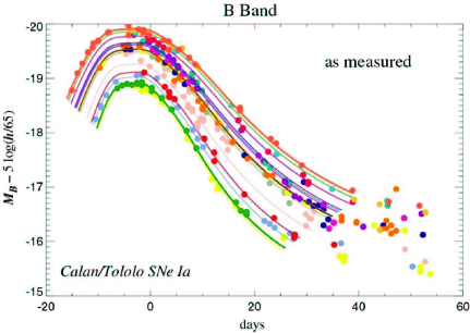
Figure 1: B-band light curves of the Calán/Tololo type-Ia supernova sample before any duration-magnitude correction.

Several empirical techniques [12, 13, 14, 15] have been developed since then to make use to this correlation to turn type-Ia SNe into standard candles, with a dispersion on their peak magnitude of only 0.10–0.15 mag, corresponding to a precision of about 5–7% in distance, and, therefore, in lookback time to the explosion. Figure 2 shows the same SNe light curves of fig. 1 after applying the “stretch” technique of [12], so called because it basically amounts to a simple stretching of the time axis, showing the good uniformity achieved.

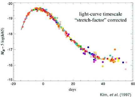
Figure 2: Same light curves of fig. 1 after applying the “stretch” duration-magnitude correction of ref. [12].

While light-curves are determined with photometric measurements in several broadband filters, spectroscopy near maximum light serves the dual purpose of unambiguously identifying the object as a type-Ia SN and at the same time determining its redshift. Both goals are achieved by comparing the measured spectrum to templated spectra from well-measured near-by type-Ia supernovae. The key feature of the spectrum is the Si-II absorption line, whose detection identifies the SN as a type Ia, and whose position determines the redshift. Figure 3 shows spectra of three supernovae: from top to bottom, a type II, a type Ia, and a type Ic . The Si-II feature can be seen clearly in the type-Ia spectrum.

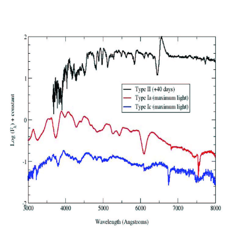
Figure 3: Measured spectra of three supernovae. From top to bottom: type II, type Ia, type Ic. The Si-II feature identifying a type-Ia SNe is clearly visible in the middle spectrum at about 600 nm.

2.2 Cosmology

Once the stretch-corrected magnitude and redshift are determined, the supernova can be put into a Hubble diagram in order to measure the cosmological parameters. The Hubble diagram is a plot of measured magnitude vs. redshift. Since the apparent magnitude of a standard candle gives us its distance and the time $t$ at which the light was emitted, and the redshift gives the cosmic expansion parameter $a(t)$, a Hubble diagram populated with SNe at different distances gives us the history of the expansion of the universe. Since the expansion rate of the universe is determined by its matter-energy content, it is clear that type-Ia SNe can tell us about the properties of the contents of the universe, and, in particular, of the dark energy component.

Assuming that the universe is homogeneous and isotropic at large scales leads to the Friedman-Lemaître-Robertson-Walker (FLRW) universe defined by the metric $\rmd s^{2}=\rmd t^{2}-a^{2}(t)(\rmd r^{2}/(1-kr^{2})+r^{2}(\rmd\theta^{2}+\sin^{2}\theta\rmd\phi^{2}))$, where $t$ is the proper time and $(r,\theta,\phi)$ are co-moving coordinates. For a flat universe, that we will assume in most of the following, $k=0$. For the FLRW metric, Einstein’s field equations of general relativity reduce to the so-called Friedman-Lemaître equations:

$$\frac{\ddot{a}}{a}=-\frac{4\pi G}{3}\left(\rho+3p\right)$$ (1)

$$\left(\frac{\dot{a}}{a}\right)^{2}=\frac{8\pi G}{3}\rho-\frac{k}{a^{2}}\ .$$ (2)

From the first equation, it is clear that in order for the expansion of the universe to accelerate ($\ddot{a}>0$), it is necessary that $\rho+3p<0$, or $w<-1/3$.

Since both $\rho$ and $p$ evolve with time, in order to solve for $a(t)$ we need an extra equation. This can be the equation of state for each component of the universe, relating its energy density with its pressure. For matter (ordinary or dark), $p=0$, so $w=0$. For radiation, we have the relativistic gas relationship $p=\rho/3$, so $w=1/3$. As mentioned before, for the cosmological constant one has $p=-\rho$, or $w=-1$. Assuming a flat universe, Eqs. (1,2) can be used to obtain the relationship

$$\frac{\rmd\rho}{\rmd a}=-3(1+w)\frac{\rho}{a}\ ,$$ (3)

from which, assuming a constant equation of state $w$, one gets:

$$\rho=\rho_{0}a^{-3(1+w)}\ ,$$ (4)

which results in $\rho=\rho_{0}a^{-3}=\rho_{0}(1+z)^{3}$ for matter, $\rho=\rho_{0}a^{-4}=\rho_{0}(1+z)^{4}$ for radiation, and $\rho=\rho_{0}$ for a cosmological constant. Introducing the Hubble parameter $H=\dot{a}/a$ and defining the critical density as $\rho_{c}=3H_{0}/8\pi G$, where $H_{0}$ is the Hubble parameter now, we can cast eq. (2) as

$$H^{2}=H^{2}_{0}\left[\Omega_{M}(1+z)^{3}+\Omega_{r}(1+z)^{4}+\Omega_{DE}(1+z)^{3(1+w_{DE})}\right]\ ,$$ (5)

where we have introduced the current normalized densities $\Omega_{i}\equiv\rho^{i}_{0}/\rho_{c}$, for $i=M$ (matter), $r$ (radiation) and $DE$ (dark energy). The term proportional to $\Omega_{r}$ can be safely neglected for all purposes, at least for moderate values of $z$ ($z<5000$). It is clear from this equation that by measuring $H$ at different times (the history of the expansion of the universe as provided by type-Ia SNe), one can learn about the properties of the constituents of the universe, $\Omega_{M},\Omega_{DE},w_{DE}$, etc.

2.3 The Hubble diagram

Standard candles (or, in the case of type-Ia SNe, “standardizable” candles) provide a measurement of the luminosity distance $d_{L}$ as a function of redshift. $d_{L}$ can be defined through the relation $\phi=\frac{L}{4\pi d_{L}^{2}}$, where $L$ is the intrinsic luminosity, and $\phi$ the flux, so that $d_{L}$ is the “equivalent distance” in a Euclidean, non-expanding universe. It is easy to see that $d_{L}(z)=(1+z)\,r(z)$, where $r(z)$ is the co-moving distance to the source at redshift $z$. Recalling that light travels in geodesics ($\rmd s^{2}=0$), we can easily compute $r(z)$ from the FLRW metric as

$$r(z)=\int_{1}^{2}\rmd r=\int_{1}^{2}\frac{\rmd t}{a}=\int_{1}^{2}\frac{\rmd a}{a\dot{a}}=\int_{0}^{z}\frac{\rmd z^{\prime}}{H(z^{\prime})}\ ,$$ (6)

where for simplicity we have assumed a flat universe. Astronomers measure fluxes as apparent magnitudes:

$$m(z)\equiv-2.5\log\left(\phi/\phi_{0}\right)={\cal M}+5\log\left[H_{0}d_{L}(z)\right]$$ (7)

$${\cal M}\equiv M+25-5\log\left[H_{0}/100\,\mathrm{kms^{-1}Mpc^{-1}}\right]\,,$$

where $M$ is the (assumed unknown) absolute magnitude of a type-Ia SN, related to $-2.5\log L$. The flux $\phi_{0}$ defines the zero point of the magnitude system used. It should become clear from eqs. (6) and (5) that, contrary to the appearances, eq. (7) does not depend on $H_{0}$. An example of a Hubble diagram can be seen in fig. 4.

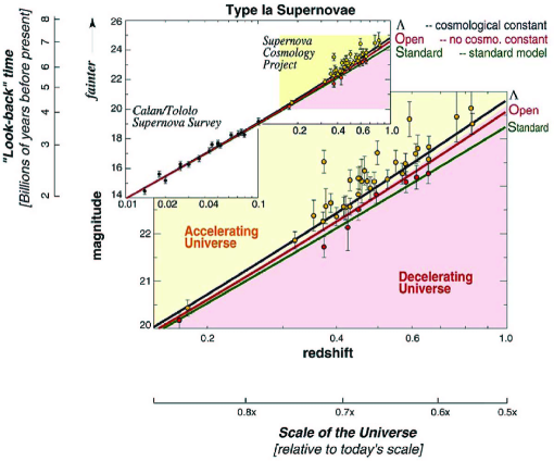
Figure 4: Example of apparent magnitude vs. redshift Hubble diagram, from the 1998 Supernova Cosmology Project results [1].

By measuring apparent magnitudes and redshifts from a set of type-Ia supernovae, one can measure different integrals of $H_{0}/H(z)$, which according to eq. (5) are sensitive to the cosmological parameters. Note that in the standard cosmological analyses ${\cal M}$ is considered a nuisance parameter and it is determined simultaneously from the data.

3 Systematic uncertainties

The statistical uncertainties in the Hubble diagram are dominated by the intrinsic supernova peak magnitude dispersion $\sigma_{\mathrm{i}nt}=0.10-0.15$. Since this error is uncorrelated from supernova to supernova, in a redshift bin with ${\cal O}(100)$ SNe (a quantity most current and all near-future surveys will achieve), the statistical error will be $\sigma_{\mathrm{s}tat}=0.01-0.02$. Since many systematic uncertainties are expected to be fully correlated for SNe at similar redshifts, but uncorrelated otherwise, it is clear that systematic errors of order a few per cent will be important, and, in many cases, already dominant.

A comprehensive study of systematic errors affecting type-Ia SNe distance measurements can be found in [16]. We will only cover the more relevant ones in the following.

3.1 Host galaxy dust extinction

Dust in the path between the supernova and the telescope attenuates the amount of light measured. Milky Way dust is well measured and understood [17], while intergalactic dust has a negligible effect. In contrast, dust in the supernova host galaxy can lead to a substantial dimming of the SN light. Ordinary dust absorbs predominantly in the blue, leading to a reddening of the SN colors. The amount of reddening can be measured, and from it, the amount of extinction can be determined, provided the extinction law (extinction as a function of wavelength) is known. The usual extinction law [18] reads:

$$m_{j}\to m_{j}+A_{V}\left(a(\lambda_{j})+\frac{b(\lambda_{j})}{R_{V}}\right)=m_{j}+E(B-V)\left(R_{V}a(\lambda_{j})+b(\lambda_{j})\right)\,,$$ (8)

where $E(B-V)$ is the excess $B-V$ color over the expected one, $R_{V}\approx 3.1$ in near-by galaxies is sometimes called the extinction law, $A_{V}=R_{V}E(B-V)$ is the increase in magnitude in the $V$ band due to dust, $a(\lambda)$ and $b(\lambda)$ are known functions, with $a(\lambda_{V})=1$, $b(\lambda_{V})=0$, and all wavelengths are in the SN rest frame. In order to correct $m_{j}$ we need to know $E(B-V)$ and $R_{V}$. The former can be determined from photometry in at least two bands. The latter is more complicated. Although it can in principle be measured directly from three-band photometry, in practice, the lever-arm is limited. Furthermore, current surveys do not have precision photometry in three bands for all their SNe. Several alternative approaches have been used in the literature. Riess et al. [5] assume $R_{V}=3.1$ everywhere; Astier et al. [3] instead determine one single effective $R_{V}$ for all their distant SNe, finding a much lower value $R_{V}=0.57\pm 0.15$. However, this parameter effectively includes any other effect that might correlate SN color and magnitude. The proposed SNAP satellite mission [19] with its nine filters will determine $R_{V}$ for each SN independently, since it will have precision optical and near-infrared photometry for all their SNe in at least three and up to nine bands. Clearly, given the uncertainties on the value of $R_{V}$ in distant galaxies, this looks like the most conservative approach.

Alternatively, surveys can restrict themselves to SNe with low extinction, signaled either by their low measured values of $E(B-V)$ or by its location in an old elliptical galaxy where star formation has long ceased and dust presence is minimal. Figure 5 shows a $w_{0}-w_{a}$ contour plane with the qualitative effect of dust correction through measurement of $A_{V}$ and $R_{V}$ from data (which increases the contour size significantly), and of uncorrected dust biases (which displace the contour).

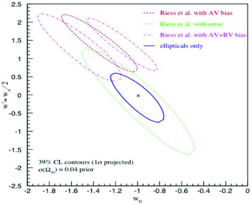
Figure 5: Example of the increase of errors due to dust extinction correction, and of biases due to uncorrected extinction.

“Gray” dust, with an effective $R_{V}\to\infty$, had been postulated as an explanation for the observed dimming of SNe at large redshift. The correction method outlined above would not work for a dust that would dim equally all wavelengths. However, natural models of gray dust would lead to dimming of all SNe at all redshifts. This has been excluded by [4, 5], which have observed SNe at redshifts beyond $z=1$ and found them to be brighter, not dimmer, than expected by models without dark energy, and in perfect agreement with the prediction of the “concordance” model: $\Omega_{M}\approx 0.25$, $\Omega_{\Lambda}\approx 0.75$.

3.2 Flux calibration

By flux calibration we understand the determination of the zero points $\phi_{0,j}$ for each filter $j$. While the overall normalization is irrelevant (since it can be absorbed in the unknown parameter ${\cal M}$ in eq. (7)), the relative filter-to-filter normalizations are crucial, as they influence, for instance, the determination of colors, which are needed for the dust-extinction corrections (as we saw in the previous section), K-corrections, etc.

The standard procedures use well-understood stars or laboratory light sources to achieve values of $\sigma_{\mathrm{c}al}$ around few per cent in flux. A complementary procedure has been presented in [20] which uses supernova data themselves to achieve a large degree of self-calibration. For example, fig. 6 show that for a fiducial survey close to the SNAP mission specifications, the procedure of [20] achieves an effective factor 5 reduction in calibration error.

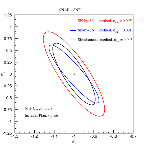
Figure 6: Effect of self-calibration in a survey similar to the one proposed by the SNAP collaboration. Using the procedure in [20] and assuming an external calibration error of 0.005 is roughly equivalent to using the standard procedure with an external error of 0.001.

4 Current surveys: SNLS

Of the current type-Ia SN surveys, the most promising is probably the SuperNova Legacy Survey (SNLS) [21], taking place at the Canadian-French-Hawaiian Telescope (CFHT) in the Mauna Kea observatory in Hawai’i. The telescope and camera provide a 3.6 m aperture, 1 deg² of field of view and a focal plane with 36 CCDs with a total of 328 million pixels. The survey team will be taking data for 40 nights per year during the 2003-2008 period in a four-night-cadence rolling search in four 1-deg² fields in the $g$, $r$, $i$, and $z$ bands. At the end of the five years the collaboration expects to have discovered and followed 500-700 type-Ia SNe with redshifts up to $z=1$. Spectroscopic follow-up of most good candidates is performed in several 10 m-class telescopes in both hemispheres: VLT, Gemini North and South, and Keck. The resulting spectroscopic time needed is comparable in size to the imaging time in CFHT. Figure 7 shows two SNe with the four light curves measured for each one. For the SN at redshift $z=0.91$ the $g$ and $r$ light-curves correspond to deep UV in the SN rest frame and, therefore, are not used in the analysis.

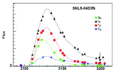
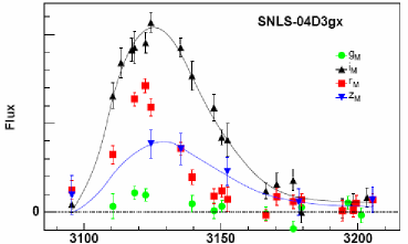
Figure 7: SNLS light curves for low- (top), and high- (bottom) redshift supernovae. For the SN at redshift $z=0.91$ the $g$ and $r$ light-curves correspond to deep UV in the SN rest frame and, therefore, are not used in the analysis. The horizontal scales are in units of days.

For each SN $i$, the SNLS light-curve fit performs K-corrections and returns the $B$ magnitude (in SN rest frame) at peak luminosity $m_{B}^{i}$, the stretch factor $s^{i}$, and the observed color excess $E^{i}(B-V)$. Every available filter is used in the fit, provided it corresponds to the $U$, $B$, $V$, $R$ regions in the SN rest frame. At least two filters for SN are required (in order to determine $E(B-V)$. The cosmology fit then proceeds as:

$$m_{B}^{i}={\cal M}_{B}+5\log[H_{0}d_{L}(z^{i},\vec{\theta})]-\alpha(s^{i}-1)+\beta E^{i}(B-V)\,,$$ (9)

where $\vec{\theta}$ are the cosmological parameters, and the nuisance parameters ${\cal M}_{B}$, $\alpha$, $\beta$ are also fitted from the data. The last two give the slopes of the dependency of the magnitude with stretch ($\alpha$) and color ($\beta$).

Analyzing 73 new high-$z$ SNe from SNLS first-year data, together with 44 previously published near-by ($z<0.1$) SNe, and including the Baryon Acoustic Oscillations measurement of [22], the SNLS team finds 68% constraints on the cosmological parameters:

$$\Omega_{M}=0.271\pm 0.022$$

$$w=-1.02\pm 0.11\,,$$ (10)

where $w$ has been assumed constant and the universe flat. Figure 8 shows the Hubble diagram corresponding to these data. The mean dispersion of the SNLS magnitudes about the best-fit prediction is only $\sigma_{\mathrm{int}}=0.12$ mag.

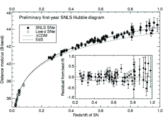
Figure 8: Hubble diagram corresponding to the SNLS first-year data, together with 44 low-$z$ SNe. Note that the average dispersion of the SNLS measured magnitudes about the best-fit prediction is only 0.12.

The SNLS also expects to gather an additional 500 or so type-Ia SNe without spectroscopic data, because of lack of resources. This highlights the problem that will be faced by the next generation of deep ground-based type-Ia SN surveys. For instance, the Dark Energy Survey (DES) plans to image about 2000 type-Ia SNe up to $z=1$ in 2010-2014. However, it seems impossible to gather the 10 m-class telescope needed to get spectra for all those SNe. Therefore, techniques have to be developed to do without spectroscopy for most of the SNe. A recent paper by SNLS [23] discusses some methods to classify SNe with just multi-color light-curve information, and to determine their photometric redshift. A 90% purity is obtained by using a real-time analysis of pre-maximum light curves (used to trigger spectroscopic follow-up). Presumably, higher purity and efficiency could be achieved by using all light-curve information. Similarly, the precision of the photometric redshifts is around $\langle|z_{\mathrm{p}hot}-z_{\mathrm{s}pec}|\rangle=0.03\cdot(1+z)$, which seems adequate for most purposes.

5 Future surveys: SNAP

Of the proposed supernova surveys in the next decade, the SuperNova Acceleration Probe (SNAP) satellite mission is probably the most ambitious. In essence, it consists of a 2 m-class wide-field (0.7 deg²) imager with state-of-the-art optical and near-infrared camera and an integral-field-unit spectrograph. The dual aim is to collect about 2000 type-Ia SNe up to redshift $z=1.7$, and to study weak gravitational lensing from space. If approved, it could fly from about 2013–2015 on.

Since a space mission is always much more expensive than a ground-based survey, the first question that comes to mind is “why space”? Figure 9 demonstrates that for a SNAP-like mission, and keeping the time of the mission constant, there is a clear advantage in sensitivity to $w_{a}$ by going to larger redshifts, $z\geq 1.5$. Furthermore, the window to the deceleration era $z>1$ can help in eliminating systematic errors (see, for instance, the gray dust discussion in section 3.1). However, for $z>1-1.2$, the rest-frame $B$ band gets redshifted into the observer near infra-red region ($\lambda>1.2\mu$m). At these wavelengths, atmospheric absorption makes it all but impossible to perform accurate measurements from the ground, hence the need for a space-based mission.

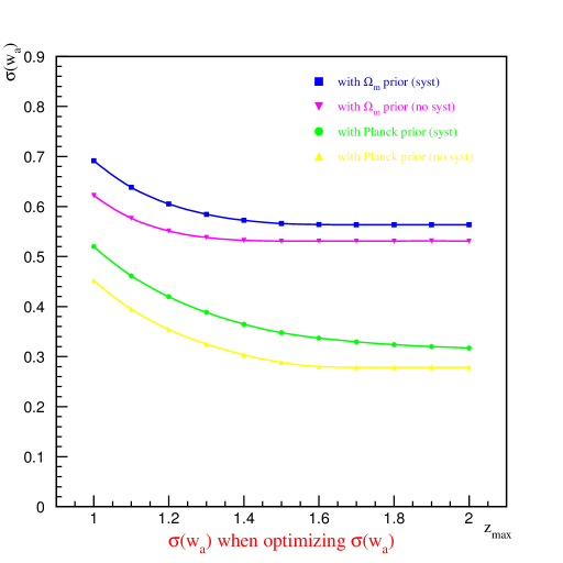
Figure 9: Uncertainty on the $w_{a}$ parameter as a function of maximum redshift $z_{\mathrm{m}ax}$ for a SNAP-like mission with fixed total time. The different lines correspond to different assumptions about priors and systematic errors.

The SNAP optical imaging system incorporates nine redshifted wide-band filters covering from the $U$ band to about 1.7 microns. The detectors are LBNL-developed thick, back-illuminated CCDs with quantum efficiency above 50% up to one micron, and HgCdTe detectors covering the near-infrared region. The nine filters ensure that at least there colors are available for all SNe in their restframe $U$ to $R$ wavelength range. This information can be used to determine the reddening law $R_{V}$ individually for each supernova, eliminating a potentially damaging systematic uncertainty.

The large number of SNe in each redshift bin will also allow to tackle the issue of “evolution” of SNe properties with redshift. This has been often mentioned as a potentially dangerous source of systematic errors. By taking multi-color light-curves and multi-epoch spectra for all the supernovae, SNAP will be able to classify them according to their observational differences. Then, cosmology can be extracted by performing cosmology fits within each sub-type, each including both low- and high-redshift SNe (“like-to-like” comparison). In practice, this is done by allowing a different value of the nuisance parameter ${\cal M}$ for each sub-type. It has been shown in [16] that the statistical degradation due to the extra free parameters in the fit is only of a few per cent.

Figure 10 shows the expected SNAP precision in the $w_{0}$–$w_{a}$ plane. SNAP with SNe and weak lensing can, by itself, determine $w_{0}$ to about 5%, and $w^{\prime}\approx w_{a}/2$ to about 10%.

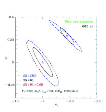
Figure 10: Expected reach of the SNAP satellite mission. The “$\Lambda$” contours correspond to assuming a $\Lambda$CDM fiducial universe, while the “S” contours correspond to a Supergravity-inspired model. The “$\Lambda$” universe tends to lead to the most conservative contours. Note in both cases the big improvement after adding weak lensing.

6 Summary

Type-Ia supernovae provided the “smoking gun” for the accelerated expansion of the universe and the existence of dark energy. It is by now a mature technique, where sources of systematic errors are better identified and understood than for most other techniques. However, it is still being perfected, and improvements happen constantly.

The control of systematic errors holds the key to any substantial future improvements. Calibration, redshift evolution of SN properties, and dust extinction corrections are the three main sources of systematic uncertainties. Current and future SN surveys address them with different levels of sophistication.

There is a vigorous current and future program of SN surveys, ranging from low-$z$ SNe from the ground (like SNF, SDSS-II/SNe, CfA, Carnegie) through medium- to high-$z$ surveys from the ground (Essence, SNLS, DES, PanSTARRS, LSST) to high-$z$ surveys from space (JDEM, DUNE).

We should expect more insight on the nature of dark energy from current and future studies of type-Ia supernova samples.

References

References

- [1] S. Perlmutter et al., Astrophys. J. 517 (1999) 565 [arXiv:astro-ph/9812133].
- [2] A. G. Riess et al., Astron. J. 116 (1998) 1009 [arXiv:astro-ph/9805201].
- [3] P. Astier et al., Astron. Astrophys. 447 (2006) 31 [arXiv:astro-ph/0510447]
- [4] R. A. Knop et al., Astrophys. J. 598 (2003) 102 [arXiv:astro-ph/0309368].
- [5] A. G. Riess et al., Astrophys. J. 607 (2004) 665 [arXiv:astro-ph/0402512].
- [6] M. Chevallier and D. Polarski, Int. J. Mod. Phys. D 10 (2001) 213 [arXiv:gr-qc/0009008].
- [7] E. V. Linder, Phys. Rev. Lett. 90 (2003) 091301 [arXiv:astro-ph/0208512].
- [8] http://snfactory.lbl.gov
- [9] M. Sako et al., In the Proceedings of 22nd Texas Symposium on Relativistic Astrophysics at Stanford University, Stanford, California, 13-17 Dec 2004, pp 1424 [arXiv:astro-ph/0504455].
- [10] D. A. Howell et al., Nature 443 (2006) 308 [arXiv:astro-ph/0609616].
- [11] M. M. Phillips, Astrophys. J. 413 (1993) L105.
- [12] S. Perlmutter et al., Astrophys. J. 483 (1997) 565 [arXiv:astro-ph/9608192].
- [13] M. Hamuy, M. M. Phillips, J. Maza, N. B. Suntzeff, R. A. Schommer and R. Aviles, Astron. J. 109 (1995) 1669.
- [14] A. G. Riess, W. H. Press and R. P. Kirshner, Astrophys. J. 473 (1996) 88 [arXiv:astro-ph/9604143].
- [15] J L. Tonry et al., Astrophys. J. 594 (2003) 1 [arXiv:astro-ph/0305008].
- [16] A. G. Kim, E. V. Linder, R. Miquel and N. Mostek, Mon. Not. Roy. Astron. Soc. 347 (2004) 909 [arXiv:astro-ph/0304509].
- [17] D. J. Schlegel, D. P. Finkbeiner and M. Davis, Astrophys. J. 500 (1998) 525 [arXiv:astro-ph/9710327].
- [18] J. A. Cardelli, G. C. Clayton and J. S. Mathis, Astrophys. J. 345 (1989) 245.
- [19] http://snap.lbl.gov
- [20] A. G. Kim and R. Miquel, Astropart. Phys. 24 (2006) 451 [arXiv:astro-ph/0508252].
- [21] http://cfht.hawaii.edu/SNLS
- [22] D. J. Eisenstein et al., Astrophys. J. 633 (2005) 560 [arXiv:astro-ph/0501171].
- [23] M. Sullivan et al., arXiv:astro-ph/0510857.